Abstract
This paper validates and presents the efficiency and performance of Synchronous Reference Frame (SRF) control as a mitigating control in managing risks of high volatility of electric current flows from the wind turbine generator to the distributed load. High volatility/fluctuations of electricity (high current, voltage disturbance) and frequency are hazards that can trip off or, in extreme cases, burn down a whole wind turbine generator. An advanced control scheme is used to control a Voltage Source Converter (VSC)-based three-phase induction generator with a Battery Energy Storage System (BESS). For the purpose of risk mitigation of harmonics, this scheme converts three-phase input quantity to two-phase Direct Current (DC) quantity (dq) so that the reactive power compensation decreases the harmonics level. Thus, no other analog filters are required to produce the reconstructed signal of fundamental frequency. In this paper, the values of Proportional Integral (PI) regulators are calculated through the “MONTE CARLO” optimization tool. Furthermore, risk analysis is carried out using bowtie, risk matrix and ALARP (as low as reasonably practicable) methods, which is the novelty based on the parametric study of this research work. The results reveal that by inducting proposed SRF control into the Wind Energy Conversion System (WECS), the risks of high fluctuations and disturbances in signals are reduced to an acceptable level as per the standards of IEEE 519-2014 and EN 50160. The proposed work is validated through running simulations in MATLAB/Simulink with and without controls.
1. Introduction
To rectify the problem and to mitigate the undesirable output of high penetration in the area of renewable energy sources such as wind, solar, biomass, etc., it is essential to get a reliable and robust solution [1]. Generating energy through standalone wind turbines, particularly in remote areas, is a tremendous source of clean and cheap energy that can meet the targets of goal number seven of the Sustainable Development Goals (SDGs) of the United Nations (UN) [2]. However, the instability of power generation and transmission of these wind turbines poses risks of volatility of frequency and harmonic distortions. This research mitigates these risks by proposing and validating the efficacy of the Synchronous Reference Frame (SRF) control scheme as an effective control, thus endorsing the application of a proposed control scheme by increasing the energy produced through standalone wind turbines and consequently playing a pivotal role in meeting the goals of the SDG of the UN. There might be changes in overall system frequency when the power generation in the system is not adequate or balanced with total demand side requirements. Fluctuations in total power generation disturbs the system frequency and causes time error. If overall generation in the system is rapidly higher than demand requirements, frequency goes up; if generation is lower than demand requirements, frequency goes down [3]. In order to mitigate the risk of these fluctuations and stabilize the overall power transmission system, a control algorithm for power system components can be used. Moreover, Monte Carlo simulation can be applied to get accurate values for controlling signals [4].
Interest in carrying out comprehensive risk assessments is growing with the development of systems and electric utilities. Over the past few years the world has witnessed many large power failures and outages. Risk of power failure and outages cannot be fully avoided because of the probabilistic characteristics of power systems. However, the system risk can be estimated and mitigated to an acceptable level in planning, designing, operational and maintenance phases [5]. Changes in load demand create fluctuations in voltage and frequency; these fluctuations and variation in wind speed are the main problems in wind generators employed in the distributed generation system. However, in recent years advanced technologies in power electronic converters have been used to mitigate the above-mentioned problems up to a certain level. For instance, advance converters are used to improve power quality as per the IEEE standards 519-2014 and European Standard EN 50160 [6,7]. Moreover, to create reference signals for controlling converters and to overcome power quality problems, an adaptive control algorithm Enhanced Phase Lock Loop (EPLL) was used in [8]. Synchronous Reference Frame (SRF, also called Clark’s transformation) theory was used in distributed power generation for the reliable operation of a power system [9,10,11]. Similarly, Lorentzian norm-based adaptive filter (LAF) was used to control the converter in a distributed generation system for better power quality issues [12]. To improve further the power quality features in standalone distributed power generation systems, frequency and voltage were regulated to set the reference value and the Variable Learning Gradient-Based (VGLMS) Least Mean Square algorithm was used in [13]. Harmonics were generated due to nonlinear and undesirable load and high switching frequency of converters that affected wind generation and the overall system. B.Singh et al. presented a control scheme with an SRF- and PLL-based strategy in [14,15,16]. For such power quality issues, reactive power compensation can be applied as in B.Singh et al., who depicted some control schemes for mitigation of this problem in [17,18,19]. Some optimization techniques were used to tune the Proportional Integral (PI) controller of the control algorithm and to get accurate values of PI gains. To get values of the PI controller, a Multi-Verse Optimization (MVO) algorithm was used in [20]. In this, Naidu et al. used it to get accurate gain values after some iterations for controlling PI and robust output. For getting fast values then MVO, Particle Swarm Optimization (PSO) was used to optimize errors between actual and reference values, and the Integrated Time Square Error (ITSE) was used as a cost function of this optimization algorithm in [21]. For robustness and better optimization than PSO and MVO, Saba raj et al. used the Whale Optimization Algorithm (WOA) in [22]. Compared to trial and error methods for tuning of the PI controller, with much less time the WOA delivers the suitable values of Proportional Integration (PI). For risk assessment and analysis of mitigation in reactive power losses and voltage instability, Jalali et al. offered a sustainable means of improving reliability and robustness of power systems in [23]. Y. Zhang et al. presented about Conditional Value-at Risk (CVaR) when wind power output has some fault and problems in [24]. The research carried out risk analysis and the impact of risk level in power systems. F. Leonardi et al. designed service robots in [25] for the inspection and maintenance of a wind plant. M. Lei et al. depicted their article about calculation of risk losses, risk values and changes caused by demand response under load curve considering wind power generation in [26]. Peng Liu et al. represented dynamic security decision trees that were based on risk measurements and power quality problems of wind generators [27]. For assessment, identification and evaluation of risks, Riccardo Mogre et al. implemented Decision Support Systems (DSSs) for supply chain (risk management), which was beneficial from a holistic approach for decreasing risks in [28].
In this paper, power quality issues and generator fire risks are assessed and evaluated in MATLAB simulation by collecting and managing data such as signal ratings, wind velocity and related problems. Furthermore, this research carries out a comprehensive risk assessment under the risk management framework of ISO 31000 2018 [29]. A bowtie risk identification tool is used in this work. The left-hand side of the bowtie represents the causes of the system along with preventive controls/barriers, whereas the right-hand side represents the consequences of the system fluctuation along with mitigating controls. A list of preventive and mitigating controls are identified through bowtie analysis in response to wind turbine power quality challenges. The list of controls is not exhaustive and further controls could be defined, but this paper does not attempt to cover all controls as well as future needs. SRF control is analyzed and assessed as a mitigating control on the right-hand side of the bowtie, as shown in Figure 1. The effectiveness of the control is depicted with dark green being the most effective and orange the least, and so on; SRF control is on the right side of the bowtie as a risk mitigating control. The effectiveness level of the SRF control is depicted as high in Figure 1 because of its proven and reliable application of mitigating power quality issues [14,15,16]. Moreover, our study also found that after applying the SRF control scheme of Section 2 of the paper, the risk mitigation results are promising, as presented in the results part of this paper. On the right side, the figure includes consequences or result of the hazards after preventive and mitigating controls. Moreover, these consequences such as “generator fire” and “load at risk”, etc. are evaluated based on risk matrixes, which are at the bottom part of the rectangle. These risk matrixes are comprised of risks of fatalities (first rectangle from left), assets (second rectangle) and environmental (third rectangle), and reputational (fourth rectangle) damages are given within the rectangle of consequences.
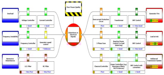
Figure 1.
Bowtie analysis of distortions in electrical signals.
Following Figure 2, the risk matrix depicts the likelihood and consequences of the risks [30]. Expected losses are an end result after applying controls are measured by the product of probability of occurrence and severity of consequence in the risk matrix [31]. These losses are categorized in risk categories of the risk expert’s opinion and author’s own judgment after applying risk controls. The prioritization of risk is presented within the risk matrix in different risk categories that show the consequence side of the bowtie [32]. This paper is analyzing risks of damages to wind turbine generators; hence, the risk matrix shows only the risk categories of damages to wind turbines presented here. For instance, there are Assets A (A0 risk category means very unlikely and no damage), Assets B (B1 category risk means unlikely and slight damage), Assets C (C2 category risk means possible and minor damage) and Assets D (D3 category risk means likely and localized damage). However, the B3 risk category shows an unlikely relationship with the consequences of localized damage after applying preventive and mitigating controls such as SRF. The likelihood of distortions, i.e., frequency fluctuations (49.5–50.2 Hz) and harmonics (below 5%), are within acceptable level of risks as analyzed, assessed and mitigated in coming sections of this paper.
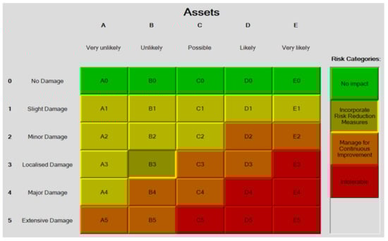
Figure 2.
Risk matrix analysis of distortions in electrical signals.
2. System Configuration
The overall structure of the proposed three-phase standalone wind-based distributed generation system is shown in Figure 3. A three-phase induction generator is coupled with a wind turbine and rotates by the horizontal axis of the wind turbine, which supplies power directly to the nonlinear load. A three-phase capacitor bank, which is star connected and shunt with a self-excited induction generator (SEIG), is used to provide external excitation to the SEIG [12]. This capacitor bank is required to supply reactive power to generate nominal voltage at no load while also working as a high frequency ripple filter. Under the linear loading condition, this capacitor bank is useful to regulate voltage and frequency without any static compensator. Under the nonlinear loading condition, total harmonics distortion, and reactive power compensation of the load current, a voltage source converter (VSC) is connected in a shunt at the point of common coupling (PCC) [12]. The VSC consists of three legs of an insulated gate bipolar transistor (IGBTs) with a dc bus capacitor (Cdc) and battery energy storage system (BESS), and a three-phase interfacing inductor (Lif) is used to convert the square output of VSC to sinusoidal output and connect to the PCC. The three-phase non-linear load is connected to the generator output which consists of a diode with resistive and inductive passive elements [13]. At the end, possible graphical representation of risk assessment is shown in the upper part of Figure 3. The remaining design parameters are depicted in the Appendix A.
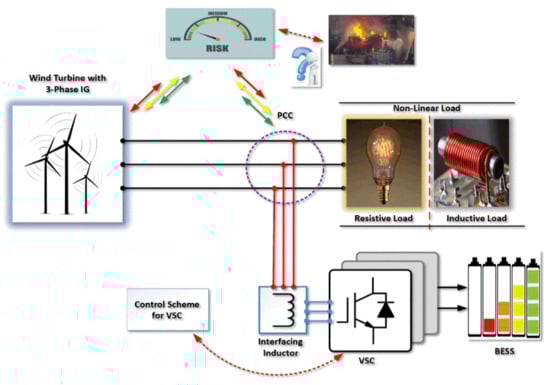
Figure 3.
Graphical representation of overall system configuration.
2.1. Control Scheme and Optimization Strategy
2.1.1. Control Scheme
SRF theory is also called “Clark’s transformation”, which transforms three-phase quantity to two-phase quantity and gives alpha and beta components as output variables [33]. To mitigate the harmonics effects in the supply voltages or currents, the conventional SRF method can be used. In this system, the load current quantities are transformed to fundamental active and reactive components (alpha-beta) with the help of Clark’s transformation sine and cosine components (from phase-locked loop (PLL)) and are used in this transformation, which are extracted from the supply voltage. After that, alpha-beta components are converted into a rotating axis which has d-q components with the help of park transformation, and eventually d-q components are converted into three-phase quantity (called inverse park transformation), which is part of reference quantity and helps to create control signals to control VSC (shown in Figure 4). The significance of d–q components is in the active and reactive quadrature axis. Three-phase quantity is rotated at the reference frame with fundamental frequency in park transformation. Here, the fundamental frequency component seems to be stationary while the signals other than the fundamental frequency seem to be oscillating. A low-pass filter is used to get the fundamental quantities of d-q current components. The d axis current component shows the current for active power. Similarly, the q axis component shows the current for reactive power. Angle theta (θ) is needed for transformations, which is calculated from PLL (phase locked loop) techniques [9]. All equations for transformations are shown in the following sections.
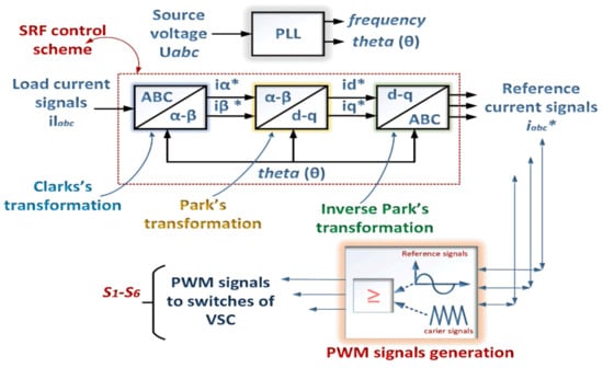
Figure 4.
Synchronous Reference Frame (SRF) control scheme.
2.1.2. Alpha-Beta (Clark’s) and d–q (Park’s) Transformation
Fundamental components of Clark’s transformation (alpha-beta) (reference current) can be calculated from the above matrix, for information about Equation [34]. Similarly, quadrative active and reactive components of Park’s transformation (d–q) (reference current) can be computed as below [34].
From Equations (1)–(3), reference current signals ia*, ib* and ic* (eventual generation of reference signals from dq* transformation) are calculated as follows:
Similarly, the p–q theory is used for power balance and for reactive power compensation to balance the overall system. By applying Clark’s transformation, fundamental components alpha-beta (voltage reference) can be calculated as follows:
From the Equation (7), active and reactive power equations are calculated as follows:
For unity power factor (UPF) in the source current, a VSC provides reactive power as per the requirements of load. However, active power is supplied by the source; by regulating the source reference signals, load balancing is achieved [34]. By using low-pass filters, this regulates PI controllers with the help of optimization techniques and the trial and error method, and the harmonics and fundamental components of current signals are extracted easily and provide feedback to the reference frame control as reference signals. After comparing reference signals with actual signals, PWM signals are generated to control VSC (explained in next section). Refer to [14] for the system’s mathematical modelling and all calculations.
2.2. “Monte Carlo” Optimization Strategy
In this system, the Monte Carlo optimization technique is used to minimize input errors of the PI controller by using the ITSE (integration time square error) objective function in the Monte Carlo simulation. Therefore, the output error of ITSE is the input error of the PI controller. Approximate tuned value (optimized) of PI controller gains such as Kpd, Kpq and Kid, Kiq are obtained by optimization. For reactive power compensation and required source current, proper tuning of the PI controller is most important (shown in Figure 5).
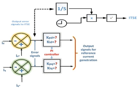
Figure 5.
Proportional Integral (PI) controller loop with Integrated Time Square Error (ITSE) objective function block.
Optimized tuned values for PI controller gains are: Kpd—0.300, Kpq—0.31, Kid—0.1 and Kiq—0.09999. Input errors are mitigated, and the PI controller is tuned after putting approximate values from optimization. After getting random values using Monte Carlo optimization techniques, a different-values graph is plotted below in Figure 6.
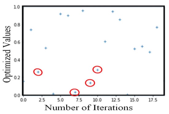
Figure 6.
Optimized values.
In Figure 6, red highlighted circles represent tuned values from optimization, which are used to tune the PI controller in this work. Moreover, the x-axis represents 20 random numbers, while the y-axis represents random values between the 0–1 range.
2.3. Role of BESS in this System
The main role of BESS is to provide support to the overall system when it is required. For instance, when power generation becomes lower than load power requirements, the battery will provide power to the load and the system will be stable. On the other hand, if power generation is higher than battery requirements, the generation power will flow towards the load first and then the rest of the generated power will flow to the battery and the battery will be charge. The total power generated by wind turbine is 12 kW in this system and there are two type of load used in this system. The load changes at 1 s and goes to 13.5 kW total power from 12 kW; at this moment, the battery is providing the remaining power to the load and the system will become stable, as shown in Figure 7. More values and parameters are explained in Appendix A.
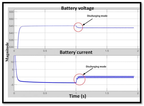
Figure 7.
Battery performance.
3. Acceptable Level of Risk Based on Results and Discussion
The overall system has been studied by the MATLAB simulation, which is depicted in Figure 3. The parameters of overall system and result’s comparisons are shown in Table 1, Table 2 and Table 3. On the other hand, simulation results with and without control at PCC are shown below in Figure 8a–d, Figure 10a–d and Figure 11. However, Figure 9 and Figure 12 shows the as low as reasonably practicable (ALARP) principle of risk analysis.
Generator current signals were distorted due to high non-linearity in the load and reactive power injected into it, while voltage signals were minimally disturbed after changing the load type from linear to nonlinear at 1 s, which is shown in Figure 8a. Moreover, Figure 8b depicts overall currents flowing in the system; the total current which is 41 A is shown on the top, whereas the middle waveform is a linear load current (18 A). The last signal is a nonlinear load current (23 A) which is connected at 1 sec. The results are without converter control because of there is a higher number of harmonics present in the signals. Perfect tuned parameters and a lower level of harmonics are acceptable in power electronics as per the industrial and standard limits (IEEE 519-2014 and EN 50160). Source voltage and current THD are acceptable below 5% [5,6].

Figure 8.
Overall results without control at point of common coupling (PCC): (a) generator voltage and current signals without control, (b) overall system current signals without control, (c) harmonics spectrum of generator voltage without control, (d) harmonics spectrum of generator current without control.

Figure 9 shows ALARP principle of risk analysis for the harmonics level, which depicts whether values are acceptable, tolerable or not acceptable. The FFT analysis and THD spectrum of generator voltage and generator current are shown in Figure 8c,d. On the other hand, Figure 10a shows that generator voltage and generator current are saturated after changing a load at 1 s because of the converter control and proper tuning of the PI controller. Figure 10b shows overall currents passing into the system, which is the generator current, and linear and non-linear load current, respectively.
Figure 10c,d shows the harmonics spectrum and analysis of generator voltage and current after applying the converter control scheme. Hence, the efficacy of this proposed control scheme is proved, as it kept the higher risk level of harmonics to an acceptable level as per IEEE standards 519-2014.

Figure 9.
As low as reasonably practicable (ALARP) diagram of harmonics level.
Figure 9.
As low as reasonably practicable (ALARP) diagram of harmonics level.


Figure 10.
Overall results without control at PCC; (a) generator voltage and current signals with control; (b) overall system current signals with control; (c) harmonics spectrum of generator voltage with control; (d) harmonics spectrum of generator current with control.
Figure 10.
Overall results without control at PCC; (a) generator voltage and current signals with control; (b) overall system current signals with control; (c) harmonics spectrum of generator voltage with control; (d) harmonics spectrum of generator current with control.

Figure 11 depicts the tracking performance of the generator current. The signal is 25% to 30% overshot at 1 s because a 50% nonlinear load is connected at this time. Settling time is within 2–3 cycles, as shown in Figure 10b. The settling time is good for the entire system it doesn’t give too much load to the power electronics controller. The values of the PI controller i.e., Kp and Ki of PI controller, are obtained by running the MC simulation as discussed in previous section. The approximate tuned values (optimized) of Kp (0.300) and Ki (0.100) gains are taken after running 20 iterations with the objective type iteration time square error (ITSE). The ITSE calculates input values and minimizes these with the square root of the output error. The low-level harmonic signals are not harmful to the generator and converter; however, it is very important to control current and voltage level at points of common coupling to avoid the fluctuations in frequency, voltage and current. A higher harmonics level could increase the heat into the generator and damage the power electronics converter. Moreover, it could also trigger distortion in signals, as shown in Figure 8c,d. Fluctuations in frequency can damage the system, however, it can be controlled by controlling voltage and the current level at the point of common coupling. A perfectly maintained level of frequency is depicted in Figure 11; it is also shown in the FFT spectrum Figure 10d after applying the control scheme.

Figure 11.
Tracking signals of reference generator current and actual generator current.
Figure 11.
Tracking signals of reference generator current and actual generator current.

Figure 12 shows the ALARP principle of risk analysis for frequency level, which depicts whether values are acceptable, tolerable or not acceptable. The above results proved the mitigation of harmonics with the control scheme based on a risk analysis. The results are based on MATLAB simulation with the 10-microsecond sampling time and variable type ode-45(dormand-prince) solver. Further system parameters, THD level and frequency values are given in Table 1, Table 2 and Table 3, respectively.

Figure 12.
ALARP diagram of frequency level.
Figure 12.
ALARP diagram of frequency level.


Table 1.
System Parameters.
Table 1.
System Parameters.
| No | Variables | Values |
|---|---|---|
| 1 | 3-phase system voltage | 325V peak to peak (400-line voltage) |
| 2 | 3-phase system current | 41 amp. total |
| 3 | 3-phase system linear-load current | 18 amp. |
| 4 | 3-phase system nonlinear-load current | 23 amp. |
| 5 | BESS voltage and current | 400 V and 150 Ah |
Table 2.
Results Comparison.
Table 2.
Results Comparison.
| No | Variables | With or Without Control | THD Values |
|---|---|---|---|
| 1 | Generator voltage | Without control | 6.80% |
| 2 | Generator current | Without control | 19.02% |
| 3 | Generator voltage | With control | 3.80% |
| 4 | Generator current | With control | 2.91% |
Table 3.
Frequency Variations.
Table 3.
Frequency Variations.
| No | Variables | With or Without Control | Values |
|---|---|---|---|
| 1 | Generator current Frequency | Without control | 49.20 Hz |
| 2 | Generator current Frequency | With control | 50.02 Hz |
4. Conclusions
This research analysis presents a control scheme by optimizing the values of PI controller gains to mitigate effects of poor power quality in a three-phase induction generator with BESS. The SRF control scheme converts three-phase quantity to two-phase vector quantity in the form of active and reactive components. It can easily control active and reactive components by proper tuning of the PI regulator. Moreover, as a controlled active and reactive quantity and tuned PI controller with optimizing techniques, all results are satisfactorily achieved with the simulation task. We also did a risk analysis in this area with some tools; for instance, the bowtie and risk matrix show criteria, such as the safe and danger zone, while getting undesirable outputs and results in the system. Risk analysis was done with the acceptable and non-acceptable power quality issues with some validated values and results.
The risk analysis with the bowtie revels all the threats that trigger an underside event of frequency, and current fluctuations are mitigated with a proposed control scheme. Risk analysis identified the acceptable and unacceptable levels of risk, and with the application of ALARP, the acceptable level of frequencies (50 Hz) and harmonic distortions (below 5%) was achieved. Moreover, running simulation in python generated random values within the acceptable range of risk. All tuned PI controller values (Kpd was 0.300, Kpq was 0.31, Kid was 0.1 and Kiq was 0.09999) were tested/simulated and verified in MATLAB.
To conclude, a control scheme for mitigation of the effects of power quality, a risk analysis when such problems occurred, optimized values of the PI controller and a risk matrix of the acceptable and non-acceptable range of the power quality problems was explained and validated through the results and discussion in the above sections.
Author Contributions
Conceptualization, S.M.; Data curation, A.Q.; Formal analysis, S.M.; Methodology, S.M.; Software, S.M. and A.Q.; Supervision, A.S.K.; Validation, S.M. and A.Q.; Writing—original draft, S.M.; Writing—review & editing, S.M. Proofreading, A.S.K., S.M. and A.Q. All authors have read and agreed to the published version of the manuscript.
Funding
This research received no external funding.
Conflicts of Interest
Authors declare that there is no conflict of interest in the research and publication of this research output.
Appendix A
- Rating and parameters of the three-phase IG: 13.3 kW, 230 V (L-G voltage, L-L 400 V), 50 Hz, and pole pair = 2. Main winding stator: Rms = 2.73 Ω, Lms = 0.0237 H. Main winding rotor: Rmr = 3.1077 Ω, Lmr = 0.0174 H. Main winding mutual inductance: Lms = 0.1379 H. Auxiliary winding stator: Ras = 5.027 Ω, Las = 0.0240 H. Inertia = 0.00291 J (kg m2). Capacitor bank = 80 μF.
- Compensator Parameters: Ls = 150 mH, rs = 0.01 Ω, cf = 1500 mF.
- BESS Parameters: 400 V (Lead-Acid), 150 Ah, SOC (70%), rs = 0.01 Ω.
Refer [14] for more system’s mathematical modelling and all calculation.
References
- Stiebler, M. Wind Energy Systems for Electric Power Generation; Springer: Berlin, Germany, 2008. [Google Scholar]
- United Nation’s Sustainable Development Goals (SDGs). Sustainable Development Goal 7. Ensure Access to Affordable, Reliable, Sustainable and Modern Energy for All. Available online: https://sdgs.un.org/goals/goal7 (accessed on 27 August 2020).
- Hong, C. Power Grid Operation in a Market Environment: Economic Efficiency and Risk Mitigation; Wiley-IEEE Press: Hoboken, NJ, USA, 2017. [Google Scholar]
- Billinton, R.; Karki, R.; Verma, A.K. Reliability and Risk Evaluation of Wind Integrated Power Systems; Springer India: New Delhi, India, 2013. [Google Scholar]
- Li, W. Risk Assessment of Power Systems; Wiley-IEEE Press: Hoboken, NJ, USA, 2014. [Google Scholar]
- IEEE Standards 519-2014. IEEE Recommended Practices and Requirements for Harmonic Control in Electric Power Systems; IEEE: Piscataway, NJ, USA, 2014. [Google Scholar]
- Markiewicz, H.; Klajn, A. Voltage Disturbances Standard EN 50160—Voltage Characteristics in Public Distribution Systems; Wroclaw University of Technology: Wroclaw, Poland, July 2004. [Google Scholar]
- Singh, B.; Chandra, A.; Al-Haddad, K. Power Quality: Problems and Mitigation Techniques; John Wiley and Sons: Hoboken, NJ, USA, 2014. [Google Scholar]
- Golestan, S.; Guerrero, J.M.; Vasquez, J.C. Three-phase PLLs: A review of recent advances. IEEE Trans. Power Electron. 2017, 32, 1894–1907. [Google Scholar] [CrossRef]
- Yepes, A.G.; Vidal, A.; Lopez, O.; Goval-Gandoy, J. Evaluation of techniques for cross-coupling decoupling between orthogonal axes in double synchronous reference frame current control. IEEE Trans. Ind. Electron. 2014, 61, 3527–3531. [Google Scholar] [CrossRef]
- Monfared, M.; Golestan, S.; Guerrero, J.M. Analysis, design, and experimental verification of a synchronous reference frame voltage control for single-phase inverters. IEEE Trans. Ind. Electron. 2014, 61, 258–269. [Google Scholar] [CrossRef]
- Giri, A.K.K.; Arya, S.R.; Maurya, R.; Babu, B.C. Power quality improvement in stand-alone seig-based distributed generation system using lorentzian norm adaptive filter. IEEE Trans. Ind. Appl. 2018, 54, 5256–5266. [Google Scholar] [CrossRef]
- Giri, A.K.; Arya, S.R.; Maurya, R.; Mehar, R. Variable learning adaptive gradient based control algorithm for voltage source converter in distributed generation. IET Renew. Power Gener. 2018, 12, 1883–1892. [Google Scholar] [CrossRef]
- Arya, S.R.; Singh, B.; Niwas, R.; Chandra, A.; Al-Haddad, K. Power quality enhancement using DSTATCOM in distributed power generation system. IEEE Trans. Ind. Appl. 2016, 52, 5203–5212. [Google Scholar] [CrossRef]
- Arya, S.R.; Singh, B. Implementation of kernel incremental meta learning algorithm in distribution static compensator. IEEE Trans. Ind. Electron. 2015, 30, 1157–1169. [Google Scholar]
- Singh, B.; Arya, S.R. Back-propagation control algorithm for power quality improvement using DSTATCOM. IEEE Trans. Ind. Electron. 2014, 61, 1204–1212. [Google Scholar] [CrossRef]
- Verma, A.K.; Singh, B. Harmonics and reactive current detection of a grid-interfaced pv generation in a distribution system. IEEE Trans. Ind. Appl. 2018, 54, 4786–4794. [Google Scholar] [CrossRef]
- Singh, A.; Singh, B.; Singh, S. Customized solution for real and reactive power compensation for small distribution systems. In Proceedings of the 7th International Conference on the European Energy Market, Madrid, Spain, 23–25 June 2010; pp. 1–6. [Google Scholar]
- Niwas, R.; Singh, B. Solid-state control for reactive power compensation and power quality improvement of wound field synchronous generator-based diesel generator sets. IET Electr. Power Appl. 2015, 9, 397–404. [Google Scholar] [CrossRef]
- Naidu, T.A.; Arya, S.R.; Maurya, R. Dynamic voltage restorer with quasi newton filter based control algorithm and optimized values of PI regulator gains. IEEE J. Emerg. Sel. Top. Power Electron. 2018, 7, 2476–2485. [Google Scholar] [CrossRef]
- Naidu, T.A.; Arya, S.R.; Maurya, R. Multi objective dynamic voltage restorer with modified EPLL control and optimized pi-controller gains. IEEE Trans. Power Electron. 2019, 34, 2181–2192. [Google Scholar] [CrossRef]
- Arya, S.R.; Maurya, R.; Naidu, T.A. Amplitude adaptive notch filter with optimized PI gains for mitigation of voltage based power quality problems. CPSS Trans. Power Electron. Appl. 2018, 3, 313–323. [Google Scholar] [CrossRef]
- Jalali, A.; Aldeen, M. Risk-based stochastic allocation of ESS to ensure voltage stability margin for distribution systems. IEEE Trans. Power Syst. 2019, 34, 1264–1277. [Google Scholar] [CrossRef]
- Zhang, Y.; Han, X.; Xu, B.; Wang, M.; Ye, P.; Pei, Y. Risk–based admissibility analysis of wind power integration into power system with energy storage system. IEEE Access 2018, 6, 57400–57413. [Google Scholar] [CrossRef]
- Leonardi, F.; Messina, F.; Santoro, C. A risk-based approach to automate preventive maintenance tasks generation by exploiting autonomous robot inspections in wind farms. IEEE Access 2019, 7, 49568–49579. [Google Scholar] [CrossRef]
- Lei, M.; Mo, S.; Wei, W.; Hua, Y.; Zhang, B. Risk assessment of demand response considering wind power generation. J. Eng. 2019, 2019, 1824–1829. [Google Scholar] [CrossRef]
- Liu, P.; Li, Z.; Zhuo, Y.; Lin, X.; Ding, S.; Khalid, M.S.; Sunday, O. Design of wind turbine dynamic trip-off risk alarming mechanism for large-scale wind farms. IEEE Trans. Sustain. Energy 2017, 8, 1668–1678. [Google Scholar] [CrossRef]
- Mogre, R.; Talluri, S.; D’Amico, F. A decision framework to mitigate supply chain risks: An application in the offshore-wind industry. IEEE Trans. Eng. Manag. 2016, 63, 316–325. [Google Scholar] [CrossRef]
- International Organization for Standardization (ISO) 31000:2018-Risk Management Principles and Guidelines. Available online: https://www.iso.org/standard/65694.html (accessed on 31 August 2020).
- Garvey, P.R.; Lansdowne, Z.F. Risk matrix: An approach for identifying, assessing, and ranking program risks. Air Force J. Logist. 1998, 22, 18–21. [Google Scholar]
- Aven, T. Risk Analysis: Assessing Uncertainties beyond Expected Values and Probabilities; Wiley: Hoboken, NJ, USA, 2008. [Google Scholar]
- CGE Risk Management Solutions. Available online: https://cgerisk.com/products/bowtiexp/ (accessed on 27 August 2020).
- Duesterhoeft, W.C.; Schulz, M.W.; Clarke, E. Determination of instantaneous currents and voltages by means of alpha, beta, and zero components. Trans. Am. Inst. Electr. Eng. 1951, 70, 1248–1255. [Google Scholar] [CrossRef]
- Singh, B.; Solanki, J. A comparison of control algorithms for DSTATCOM. IEEE Trans. Ind. Electr. 2009, 56, 2738–2745. [Google Scholar] [CrossRef]


© 2020 by the authors. Licensee MDPI, Basel, Switzerland. This article is an open access article distributed under the terms and conditions of the Creative Commons Attribution (CC BY) license (http://creativecommons.org/licenses/by/4.0/).