Article

Robust Enough? Exploring Temperature-Constrained Energy Transition Pathways under Climate Uncertainty

1
IFP Energies Nouvelles, 1–4 Avenue de Bois-Préau, 92852 Rueil-Malmaison, France
2
GERAD and Department of Decision Sciences, HEC Montréal, Montreal, QC H3T 2A7, Canada
*
Author to whom correspondence should be addressed.
These authors contributed equally to this work.
Energies 2021, 14(24), 8595; https://doi.org/10.3390/en14248595
Submission received: 10 November 2021 / Revised: 4 December 2021 / Accepted: 10 December 2021 / Published: 20 December 2021
(This article belongs to the Special Issue Decision Making in Energy Systems)

Abstract

:
In this paper, we study how uncertainties weighing on the climate system impact the optimal technological pathways the world energy system should take to comply with stringent mitigation objectives. We use the TIAM-World model that relies on the TIMES modelling approach. Its climate module is inspired by the DICE model. Using robust optimization techniques, we assess the impact of the climate system parameter uncertainty on energy transition pathways under various climate constraints. Unlike other studies we consider all the climate system parameters which is of primary importance since: (i) parameters and outcomes of climate models are all inherently uncertain (parametric uncertainty); and (ii) the simplified models at stake summarize phenomena that are by nature complex and non-linear in a few, sometimes linear, equations so that structural uncertainty is also a major issue. The use of robust optimization allows us to identify economic energy transition pathways under climate constraints for which the outcome scenarios remain relevant for any realization of the climate parameters. In this sense, transition pathways are made robust. We find that the abatement strategies are quite different between the two temperature targets. The most stringent one is reached by investing massively in carbon removal technologies such as bioenergy with carbon capture and storage (BECCS) which have yields much lower than traditional fossil fuelled technologies.

1. Introduction

According to the current status of scientific knowledge, one can assume, with a high level of confidence, that (i) global warming of the Earth is happening, (ii) anthropogenic greenhouse gas (GHG) emissions are to a large extent responsible of this warming [1] and, therefore, (iii) GHG emissions from human activities must be mitigated to prevent important damages on ecosystems [2], to the extent possible to the level of 1.5 °C [3].
To support the design of climate mitigation targets and policies, and especially to analyze energy transition pathways ensuring a strong abatement of GHG emissions, one may rely on an integrated assessment (IA) approach. The latter typically combines the socio-economic elements that drive GHG emissions with the geophysical and environmental elements that determine climate changes and their impacts. Integrated assessment models (IAMs) are computational tools to perform IA. Examples of such models include: BaHaMa [4,5,6], DICE [7], FUND [8], MERGE [9], PAGE [10] and TIAM-World [11]. IAMs operate under different paradigms (e.g., bottom-up or top-down, optimization, or simulation). Furthermore, they specifically vary with respect to the level of modelling details for the mitigation options. At both ends of the spectrum, the top-down model DICE aggregates all mitigation options into a single cost function, whereas the bottom-up TIAM-World model (following the TIMES paradigm of the International Energy Agency [12]) offers a technology-rich representation of the energy sector with thousands of energy technologies. This large variety of IAMs used, along with our current imperfect knowledge of all the climate change mechanisms, yield to very different GHG emissions abatement pathways (Figure 1). As a consequence, climate policy recommendations may widely vary across studies. For instance, Stern (2007, [13]) has advocated using PAGE for immediate actions to abate GHG emissions. Conversely, Nordhaus (2008, [14]), with his DICE model, has reached the conclusion that immediate and massive actions are not necessary.
This large variance in outputs across models led some economists to consider the use of current IAMs with caution [17,18,19]. Indeed, the long-term energy–economy–climate outlook provided by current IAMs is clouded with a great degree of uncertainty that may deeply affect the relevance of the policy analyses performed and the validity of the policy recommendations formulated. This is mostly due to the multiple sources of uncertainty (see for instance [20,21]), ranging from cross-models structural uncertainty (the modelling paradigms and their underlying simplifications) to within-models parametric uncertainty (because models are calibrated with imperfectly known data—measures uncertainty, and because of numerical assumptions about the future—radical uncertainty).
Therefore, dealing with risk and uncertainty in IAMs is a crucial question, both for scientists and policy makers [22]. This general question has a long history and has led to a substantial body of literature. Several approaches have been followed so far, with applications to different sectors of IAMs. Deterministic multi-scenario analysis, sensitivity analysis and Monte-Carlo simulations, stochastic programming, and stochastic control have been applied e.g., to uncertainty surrounding technology pathways [23] or economic growth [24]. In the specific case of climate modelling within IAMs, Refs. [25,26] identifythe following main streams to handle uncertainty: discrete scenario-based modelling [27], real options analysis [28] and stochastic dynamic programming/control [29,30]. As a subset of this last category, authors have also developed dedicated closed-form IAMs to integrate uncertainty [31]. To these techniques, we can add multi-ensemble uncertainty analysis where a large number of deterministic model outcomes are treated statistically [32].
These approaches prove useful, but all have drawbacks, and their implementation largely depends on the structure and size of the model at stake. Sensitivity analysis and Monte-Carlo simulations make way for the investigation of the impact of particular parameters, but do not provide unambiguous hedging strategies. Crost and Traeger [33] demonstrate that for this reason, there is no equivalence between the two approaches. Deterministic multi-scenario analysis results are also difficult to interpret as models are run in a deterministic way with little possibility to apply any probability distribution to the set of scenarios. One of stochastic programming drawbacks is that probability distributions have to be defined over the whole tree and that conclusions might be (extremely) sensitive to the choice of scenario and branching scheme. Moreover, stochastic programming may considerably increase the size of the problem to be solved, leading quickly to excessive computational times. Computational burden also typically limits the use of stochastic control approaches in IAMs.
The topic of uncertainty in integrated assessment is still on the scientific agenda, since it questions the relevance of the outcomes [34]. In this paper, we aim at contributing to the literature stream of analyzing climate uncertainty in IAMs by introducing robust optimization (RO) in a large scale, surplus maximization IAM.
Early developments of RO date back to Soyster [35], who initiated an approach to obtain relevant (feasible) solutions of linear optimization problems although matrix coefficients are inexact. They initiated this work because of one observation: even small variations in data can impact feasibility or optimality properties of a solution [36]. This idea has then been largely explored with different formalisms [37,38] or by generalizing the Soyster approach [39]. RO allows to solve decision-making problems under uncertainty even when the underlying probabilities are not known—only assumptions of the bounds of the support are required. It consists in immunizing a solution against adverse realizations of uncertain parameters within given uncertainty sets. The basic requirement for a robust solution is that constraints of the problem are not violated regardless of the realization of the parameters in the set. The issue then consists in identifying computable robust counterparts for the initial optimization program. Ben-Tal et al. [40] or Bertsimas et al. [41] review techniques for building such robust counterparts in general cases.
Up until now, RO has rarely been used in energy models [42], and even less in IAMs, with the exceptions of Babonneau et al. [43] and Andrey et al. [44]. On the other hand, the uncertainty of some climate parameters has already been studied, see, for instance, [45] for an application based on stochastic programming to analyze climate sensitivity, or [46] for a research focusing on atmospheric CO 2 concentration and using a maximin regret criterion in a linear model. Therefore, to the best of our knowledge, we propose the first application of robust optimization to a systematic analysis of uncertainty in climate model parameters of a large scale IAM. Although both the TIAM-World model and the robust optimization approach are well established, the novelty of this work lies with the application of RO to analyze the impact of climate uncertainty on IAMs results. Our hope is that, in the future, such techniques become part of the modelling toolbox accessible to decision-makers, in order to incorporate uncertainty in investment or policy decisions in a more systematic way.
A first contribution of our paper is to propose a general robust approach to consider uncertainty in simple climate models (SCMs) typically used by IAMs to represent climate evolution. Our approach relies on Bertsimas and Sim [39]. It consists in defining an uncertainty budget to control the degree of pessimism; in short, to limit the number of climate parameters allowed to deviate from their nominal values. We then obtain robust strategies by using a decomposition scheme that involve solving a series of sightly modified versions of the deterministic IAM. In comparison, Babonneau et al. [43] use robust optimization in order to protect the total future energy supply from possible perturbations of technological efficiencies. Their methodology exploits independence and first moment information about some underlying efficiency factors that have linear effects on the total available capacity for each period. Their proposed solution scheme relies on second order cone programming which might limit the size of the problems that can be efficiently addressed. More recently, Andrey et al. [44] also choose to robustify total future energy supply but make use of the budgeted uncertainty set of Bertsimas and Sim [39]. In contrast with these two approaches, our research focuses on how to robustify the world’s capacity to meet its targets regarding future temperature levels given the current available knowledge of the climate parameters. Moreover, our analysis will account for plausible perturbations of these parameters which have strong non-linear (instead of linear) effects on the temperature that will be reached. Finally, the solution scheme we propose has a similar advantage as the method of Andrey et al. [44]—to preserve the linear structure of the IAM model that needs to be solved—through a constraint generation algorithm.
The second contribution of this work is on the quantitative side. Our approach is implemented in the TIAM-World [47] integrated assessment model, which also relies on a SCM. We first define plausible uncertainty ranges for the climate parameters of the TIAM-World model and then calibrate these ranges using existing literature [48] against climate simulations from the MAGICC model [49]. Then, using a robust counterpart of TIAM-World, we enrich the climate debate by defining robust energy transition pathways for different global warming targets. In other words, we identify economic transition pathways under climate constraints for which the outcome scenarios remain relevant for any realization of the climate parameters. Moreover, we can assess which climate parameter or which combination of climate parameters are the most sensitive in our model and we can quantify the uncertainty cost. The originality of our results is that (i) unlike other studies e.g., [50,51], we consider uncertainty on all the climate system parameters of our IAM and (ii) we assess the cost of different protection levels and their impact on energy transition pathways.
The remainder of this paper is organized as follows: in Section 2, we first present the approach in the general case (for all IAMs). We then describe briefly, in Section 3, how we implement our RO approach in the TIAM-World model and, finally, in Section 4, we present numerical results of selected scenarios and review the different insights brought by the RO approach and how it can inform policy makers.

2. General Approach for Robustifying Optimization-Based IAMs

2.1. Integrated Assessment Modelling—A Stylised Description in the Optimization Framework

Integrated assessment models (IAMs) present different levels of integration [52]. On one end of the spectrum, there are models, such as the MIT IGSM [53], composed of loosely interconnected but more detailed (economic and climate, in particular) modules. At the other end, there are more integrated models such as, among others, TIAM-World, IMACLIM [54], MESSAGE [55], WITCH [56].
In this presentation, we focus on IAMs that can be cast, in compact form, as a single mathematical programming model, where a social planner would be assumed to maximize total surplus (the sum of producers and consumers surpluses, f), under constraints which could be economic, technical, or social (g), as well as climatic (h):
max x f ( x ) ( total surplus ) s . t . g ( x ) 0 ( economic , technical or social constraints ) h ( x ) 0 ( climatic constraints ) x R n
The set h ( x ) 0 of climatic constraints minimally (i) describes the Earth’s carbon cycle to determine the atmospheric CO 2 concentration; (ii) computes, using this concentration as well as other GHGs concentration (often exogenous), the Earth’s radiative forcing balance; and (iii) determines the evolution of the Earth’s mean surface temperature. This constitutes the typical climate module of well-known IAMs, such as DICE, FUND, and MERGE. We shall refer to such a module as a simple climate model (SCM). By contrast, there are more complex climate models called Earth System Models of Intermediate Complexity (EMICs), such as C-GOLDSTEIN [57], which could take hours to run, or even full-fledged climate models called Atmosphere-Ocean Global Circulation Models (AOGCMs, see, e.g., [58]), which could take weeks to run on a supercomputer.
In SCMs, the carbon cycle can be modelled in two main ways. It can be represented by different ‘carbon boxes’ (e.g., the atmosphere, the upper ocean and the lower ocean) with exchange rates, as in DICE (see Figure 2). Or it can be represented by an impulse-response function as in FUND and MERGE. In the sequel of this article, we focus on the first one. Most SCMs do not have retro-actions of the CO 2 concentration on the carbon cycle parameters, although the phenomenon is known to be of importance [59,60]. This is an obvious simplification as the CO 2 removal rate from the atmosphere is not constant due the finite uptake capacity of the ocean.
In the Dice-like SCMs, the concentration of gas g in period t in the n different compartments of the biosphere, M g ( t ) , may be expressed as a recursive equation:
M g ( t ) = T r g M g ( t 1 ) , M g ( t ) R + n
where T r g is a square matrix containing the transfer coefficients across compartments.
The modelling of radiative forcing (F) is rather similar across SCMs. It is defined by the radiative forcing of each GHG considered ( F GHG ):
F ( t ) = GHG F GHG ( t )
Radiative forcing due to CO 2 is often defined by a logarithmic function of the actual atmospheric CO 2 concentration (M):
F CO 2 ( t ) = γ log 2 M ( t ) M 0
This logarithmic function is sometimes linearized, as in TIAM-World. The main differences among SCMs are parameter values (e.g., γ and M 0 ) and the treatment of non-carbon dioxide GHGs (exogenously or not).
Change in radiative forcing translates in changes for the mean surface temperature ( T a t ) and the mean (deep) ocean temperature ( T o c ) depending in particular on the assumed climate sensitivity. In SCMs, this is generally estimated using two linear equations:
T a t ( t ) = μ F ( t ) , T a t ( t 1 ) , T o c ( t 1 )
T o c ( t ) = ψ T a t ( t 1 ) , T o c ( t 1 )
The main differences among SCMs are, again, parameter values and the functional form of μ and ψ .

2.2. The Robust IAM for Climate Parameters

Let us consider again our basic IAM formulation:
( P ) : max x f ( x ) s . t . g ( x ) 0 h ( x , a ) 0
where x R n is a vector of decision variables, and a R m is a vector of uncertain parameters in h ( x , a ) . In what follows, h will be a temperature constraint. We assume that any realization a i might take one of three values { a i , a ¯ i , a i + } , each representing the lowest value, nominal value, and highest value, respectively. This uncertainty typically gives rise to the following space of possible candidates for a:  
U = a m | z + { 0 , 1 } m , z { 0 , 1 } m , z + + z 1 , a i = a ¯ i + ( a i + a ¯ i ) z + + ( a i a ¯ i ) z
Following Bertsimas and Sim [39], it is possible to control the degree of pessimism of the solution by allowing only a subset of parameters to deviate from their nominal values. The concept of the uncertainty budget is based on the fact that it is highly unlikely that all the parameters take one of their two extreme values at the same time. This motivates the use of the following robust counterpart of the initial problem:
( R C ) : max f ( x ) s . t . g ( x ) 0 h ( x , a ) 0 , a U ( Γ )
with
U ( Γ ) = a m | z + { 0 , 1 } m , z { 0 , 1 } m , z + + z 1 , i z i + + z i Γ a i = a ¯ i + ( a i + a ¯ i ) z i + + ( a i a ¯ i ) z i
where Γ { 0 , 1 , 2 , , n } is the maximum number of parameters taking one of their extreme values. The idea behind the robustification of h is that the solution of the energy–economy problem should be feasible for any ‘nature-controlled’ realization of the uncertain parameters in, e.g., the temperature constraint. Thus, we want to identify the worst-case combination of parameters in h constrained by the uncertainty budget Γ . For example, assuming we want to determine optimal economic mitigation choices to limit global warming below 2 °C, we need to identify trajectories that meet the temperature target even though some of the climate parameters were wrongly estimated. We assume that decisions shall be taken before the actual values of the parameters are known, to reflect the current status of political discussions and scientific progress in climate science.
Under linearity conditions of h ( x , a ) with respect to a, the uncertainty set U ( Γ ) can be equivalently replaced with its convex hull (refer to example 14.3.2.B in [61] for a proof of this representation):
U ( Γ ) = a m | z + [ 0 , 1 ] m , z [ 0 , 1 ] m , z + + z 1 , i z i + + z i Γ a i = a ¯ i + ( a i + a ¯ i ) z + + ( a i a ¯ i ) z
and the robust constraint can be reformulated using strong duality as:
h ( x , a ¯ ) + i max ( a i a ¯ i ) h i ( x ) v ; 0 ; ( a i + a ¯ i ) h i ( x ) v + Γ v 0 v 0
where v is an additional decision variable that need to be optimized jointly with x, and where h i ( x ) is the derivative of h ( x , a ) with respect to a i .
The robust problem can then be reformulated by incorporating this new set of constraints in the original problem (see [39] for the original discussion about such a reformulation). Unfortunately, such reformulations are not always possible. Beyond the strictly linear case, Ben-Tal et al. [40] proposes a methodology to reformulate robust programs in the more general case of non-linear but still convex constraints when using convex uncertainty sets such as U ( Γ ) . Yet, these conditions typically involve that both h ( x , a ) be concave in a and that the uncertainty set be a convex set. The mere fact that h ( x , a ) be a concave function prevents one from replacing U ( Γ ) with its convex hull. This implies that such reformulations are unlikely to be obtainable for robust non-linear climate constraints when an uncertainty set as U is used.
As an illustration, let us consider that temperature follows some linear dynamics, i.e., Equation (5) can be written as:
T a t ( t ) = a 1 F ( t ) + a 2 T a t ( t 1 ) + a 3 T o c ( t 1 ) ,
where ( a 1 , a 2 , a 3 ) are three parameters that might be considered uncertain. When unfolding this expression in order to assess the long term effect of the parameters on the temperature level, we obtain expressions of the form:
T a t ( t ) = τ = 1 t a 2 t τ a 1 F ( τ ) + a 2 t T a t ( 0 ) + τ = 1 t a 2 t τ a 3 T o c ( τ ) ,
which is a polynomial function of ( a 1 , a 2 , a 3 ) and does not in general satisfy structural assumptions, such as monotonicity, convexity, or concavity. This makes the hope of obtaining a compact reformulation as in (9) somewhat unrealistic.
Note that it is possible to avoid the need of a compact reformulation by including additional constraints that exhaustively enumerate all possible combination of deviations that need to be verified for a given choice of Γ . Unfortunately, the number of such combinations increases exponentially with respect to m, the number of uncertain parameters. To avoid the exponential growth in the problem size, we suggest employing a constraint generation method that will attempt to identify a small subset of such extreme value combinations that are sufficient to obtain the optimal robust solution of the problem. This approach is fairly generic as it relies entirely on two modest (as we will see) assumptions: (i) the ability to identify a worst-case combination of extreme value for a fixed decision x; and (ii) the ability to solve the RC problem where the robust constraint is replaced by:
h ( x , a ) 0 , a { a ^ 1 , a ^ 2 , , a ^ K }
Let us now detail our proposed constraint generation algorithm (Algorithm 1):
Algorithm 1: Constraint generation algorithm.
Energies 14 08595 i001

2.3. Obtaining Uncertainty Ranges for Climate Parameters

The robust problem described above will require the estimation of deviation bounds for the climate parameters. Differences among SCMs especially come from their choices of these key assumptions. It is thus important to define ‘appropriate’ uncertainty ranges for those. This will help assess how robust SCMs are and understand which parameters or combinations of parameters are the most sensitive. Evaluating such ranges reveals several difficulties see for example [62,63,64]. First, as already mentioned, SCMs are designed to evaluate climate responses with limited computational burdens. They thus rely on some structural simplifications. For instance, most SCMs ignore carbon and climate feedbacks in their description of the carbon dynamics. Such simplifications induce bias. As an illustration, van Vuuren et al. [48] show how differently carbon cycle can behave within a standard impulse-response experiment, depending on whether it includes or not feedbacks. Second, there is a parametric uncertainty due to the intrinsic volatility of the natural phenomena at stake, as well as the imperfection of measures and statistical estimations. As an illustration, Knutti and Hegerl [65] exhibits different distributions and ranges for the climate sensitivity based on different lines of evidence. Additionally, third, there is a form of ‘selection bias’ due to heterogeneous degrees of information on parameters estimation and calibration. Overall, IAM-SCMs modellers may have a tendency to pay more attention to some parameters, based on available information.
Based on the previous stylized description of SCMs, one may distinguish three sets of parameters whose uncertainty has to be estimated. First, one group contains the parameters for the carbon cycle. The terrestrial carbon cycle itself is a rather large field of study in geophysics (see, e.g., [59,60] for a multi-model approach). One can also find sensitivity analysis on the carbon cycle in IAM-based research [62,64], or at least clues on how uncertain these parameters are [14]. One way of assessing the behavior of carbon cycle models is to perform the so-called ‘doubling experiment’, where the evolution of an atmospheric CO 2 doubling-concentration pulse in year 0 is followed across the various carbon sinks for the next 100–400 years. Existing multi-models experiments [48,60] point out large response spectra; Ref. [48] additionally show that simple carbon models (few boxes, simple linear recursive dynamics) such as DICE have, compared to the rest, relatively optimistic carbon cycles. Such an experiment seems to be a good starting point to calibrate a carbon cycle. However, the uncertainty it translates covers both parametric and structural uncertainty. For example, Ref. [48] argues that the PAGE model behaves very differently from the rest of the test population because it includes feedbacks on the carbon cycle. This limitation—carbon cycle models have different structures, hence different parameters—makes it difficult to adopt such a calibration procedure. Therefore, in the following application, we adopt a calibration procedure similar to that of [66], but for the four IPCC-RCP emissions scenarios ran under the multi-ensemble simulation mode of MAGICC6 [49].
A second set of parameters includes the forcing and climate sensitivities, which are likely to be the most well-documented parameters in the climate literature. They describe the global equilibrium surface forcing and warming after a doubling of atmospheric CO 2 concentration; any climate models includes these parameters. The importance of the equilibrium radiative forcing is widely acknowledged [67]; multi-models comparisons and simulations are also frequent [68]. If issues such as climate feedbacks arise in the estimation of forcing [69], available comparisons indicate plausible range for the forcing parameters (using doubling or quadrupling experiments), with the last IPCC report (AR5-WG1, [70]) providing a central value of 3.7 with a +/−0.8 99% confidence interval. This estimation is consistent with [71], and is retained for this study. Ref. [65] synthesizes plausible sensitivity ranges for the climate sensitivity for different lines of evidence, and demonstrate how critical it is if the policy objective is to prevent damages caused by certain levels of warming. The IPCC most likely value and upper bound are 3 °C and 4.5 °C, respectively, which is consistent with other papers, such as [50]. Ref. [64] makes a different choice, and end up with a range (upper bound of 8 °C) closer to what [65] refer to as ‘expert elicitation’. Combining different lines of evidence, these authors obtain a range close to the one of IPCC, which we will retain as a basis. Compared to existing literature on IAM-SCM sensitivity analysis in [64], these ranges are high for forcing and low for the climate sensitivity.
Finally, parameters entering the temperature dynamics, are part of a third group apparently less studied. By default, we proceed as [64], and apply a 10% variation to the annual heat transfer coefficients. The range of temperature responses of TIAM-World are compared against MAGICC6 for the 4 RCPs scenarios, accounting for the uncertainty of all parameters.

3. Application to TIAM-World
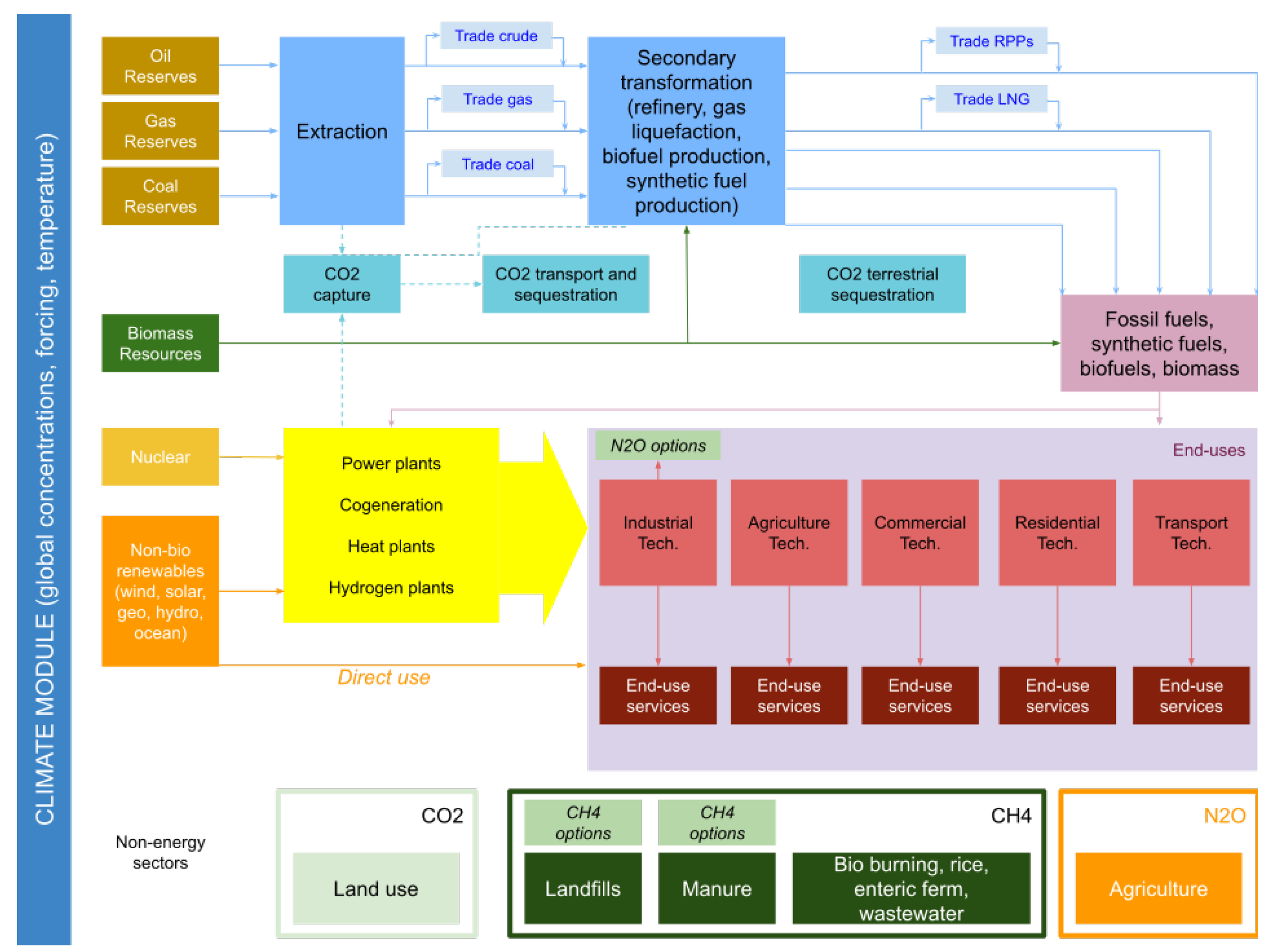
3.1. Model Overview

The TIMES Integrated Assessment Model (TIAM-World) is a detailed, global, multi-region technology-rich model of the energy/emission system of the world. It is based on the The Integrated MARKAL-EFOM System (TIMES) economic paradigm, which computes an inter-temporal dynamic partial equilibrium on energy and emission markets based on the maximization of total surplus. A complete description of the TIMES equations appears in www.etsap.org/documentation. TIAM-World is described in [11,47]. It is used in many international and European projects (for recent applications, see [43,72]). See also Appendix A for a detailed overview of the model.
The nominal formulation of the TIAM problem is a cost minimization and can be written as follows (with some simplifications):
min t c t T x t s . t . L t x t b t , x t R n , L t R m n , ( technological constraints ) D t x t d t , x t R n , D t R d n , ( demand constraints ) y t w t , with y t = A y t 1 + F x t , ( recursive climate constraints ) x t R n , y t R w , A R w * w , F R w * n
The objective function is the total cost of the system. It includes, among others: investment costs, operating costs of the various sectors, taxes, transportation costs between geographical zones. Technological constraints cover capacity limits, supply limits, yields, the allowed growth rates of the processes in the various sectors. Demand constraints include each zone’s energy service demands and climate constraints embrace limits on GHG emissions or stocks in the atmosphere or on temperature increase. These latter constraints belong to an endogenous climate module. Note that the CO 2 , CH 4 , and N 2 O emissions related to the energy sector are explicitly represented by the energy technologies included in the model. The non-energy-related CO 2 , CH 4 and N 2 O emissions (landfills, manure, rice paddies, enteric fermentation, waste water, and land use) are also included in order to correctly represent the radiative forcing induced by them, but they are exogenously defined. Emissions from some Kyoto gases (CFCs, HFCs, and SF6) are not explicitly modelled, but a special radiative forcing term is added in the climate module.

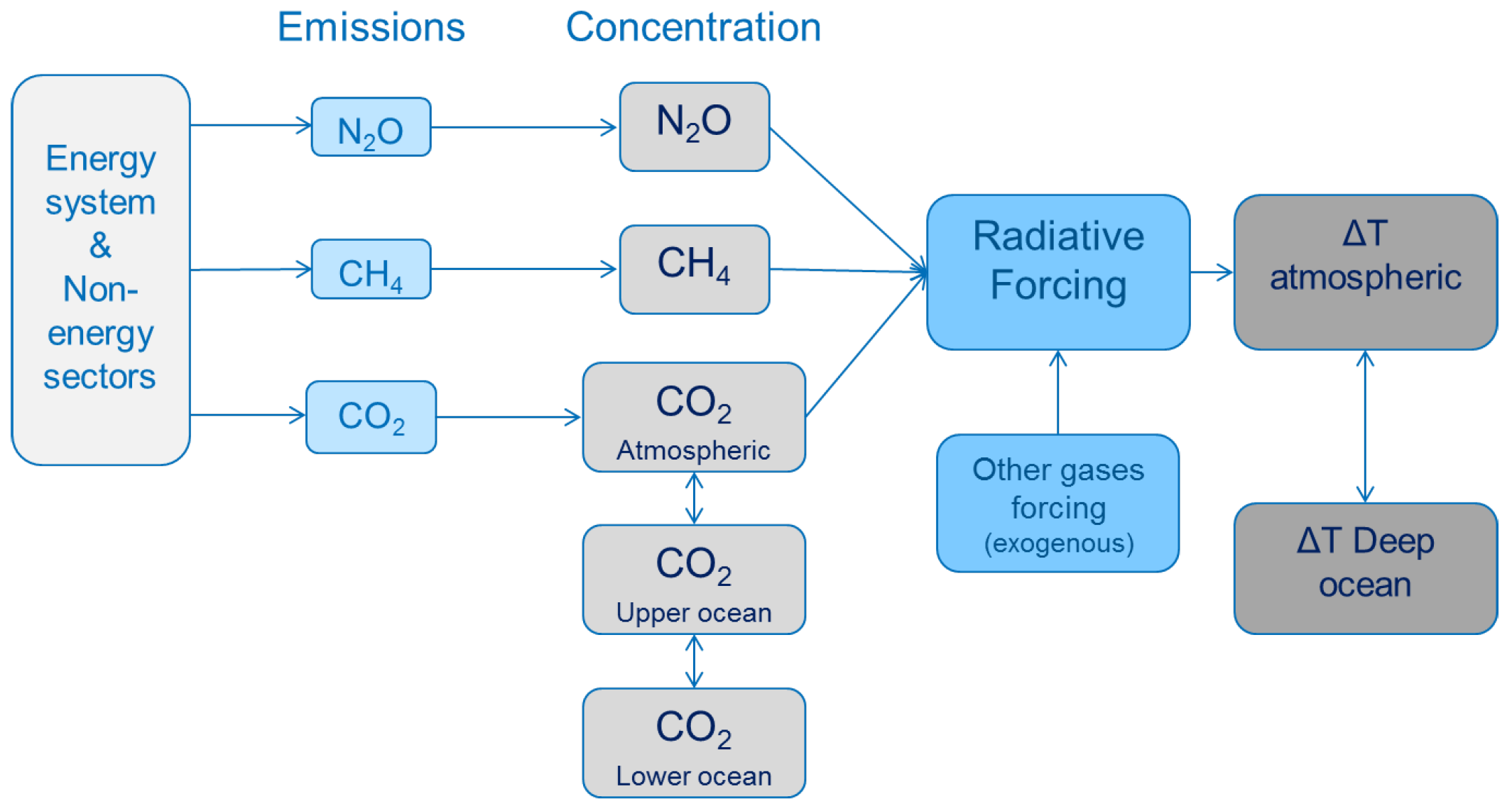
3.2. The Climate Module and the Uncertainty Sets of Climate Parameters

The climate module used in TIAM-World for this work is an adapted version of the model developed by Nordhaus and Boyer [73]. Greenhouse gas concentration and temperature changes are calculated from linear recursive equations. We briefly present its characteristics here (and in more detail in Appendix B, a detailed description can be found in Loulou et al. [74].
The climate representation in TIAM-World is characterized by three steps. First, the GHGs emitted by anthropogenic activities accumulate in the atmosphere; exchanges with the upper and deep ocean layers occur then for CO 2 , while the dissipation of CH 4 and N 2 O is described with single atmospheric decay parameters. Nine parameters populate the climate module: four carbon transfer coefficients controlling carbon dioxide exchanges between the atmosphere and the upper layer of the ocean and between the upper layer and the lower layer of the ocean ( ϕ a u , ϕ u a , ϕ l u , ϕ u l ), the radiative forcing sensitivity to atmospheric CO 2 doubling ( γ ), the climate sensitivity, i.e., the change in equilibrium atmospheric temperature due to a doubling of GHG concentration ( C S ); the adjustment speed for atmospheric temperature ( σ 1 ), the adjustment speed for oceanic temperature ( σ 3 ) and the heat loss coefficient from the atmosphere to the deep ocean ( σ 2 ).
The concrete procedure for estimating min and max values for the climate system parameters differs across parameters. Although most estimations are based on comparisons with existing literature [64,70], the construction of lower and upper bounds for the three-box carbon cycle parameters relies on a calibration against existing emission scenarios and the subsequent concentrations from MAGICC6 [49]. More detail about the estimation procedures can be found in Appendix C; Table 1 lists the nominal values and upper/lower bounds for the TIAM climate model parameters. Instead of keeping an upper and a lower value for the parameters, a rapid pre-study provided us the worst-case value of the parameters.

3.3. Robust Formulation of the Climate Problem

Based on the uncertainty that was described above, one can describe a robust counterpart of TIAM as follows:
min x t c t T x t s . t . L t x t b t , t ( technological constraints ) D t x t d t , t ( demand constraints ) y t ( x , A , F ) w t , ( A , F ) U ( Γ ) , t ( robust temperature constraints ) x R + n
where the climate equation is written as:
y t ( x , A , F ) = τ = 1 t A t τ F x τ + A t y 0
and where intuitively the uncertainty set U ( Γ ) includes any pair of matrices ( A , F ) that can be obtained by setting less than Γ of the uncertain parameters described in Table 1 to one of their extreme values. The algorithm described in Section 2.2 can be applied here as long as we are able to solve:
( S P ( x k * ) ) : { max ( A , F ) U ( Γ ) h ( x k * , A , F ) : = max t = 1 , , T y t ( x , A , F ) w t ,
and return the maximum value with a pair ( A k * , F k * ) that achieves this worst-case value for one of the time period in the horizon t = 1 , , T .
This resolution will be done by enumerating through all t’s and identifying a worst-case ( A t * , F t * ) pair for:
max ( A , F ) U ( Γ ) y t ( x , A , F ) w t .
Given that the largest worst-case difference among all t’s is achieved at t * , the oracle will return h k * : = y t ( x , A , F ) w t with the pair ( A t * * , F t * * ) to be included in M P ( U ^ ) . Although it might be possible to solve problem (11) by enumerating through all the possible scenarios for A and B, we present in Appendix D the procedure that we employed. It relies on the resolution of a mixed integer linear program which we believe should be more efficient when the number of uncertain parameters becomes large.

4. Results and Discussion

This section presents the results obtained with our robust version of TIAM-World. The uncertainty sets are given in Section 3.2 and the uncertainty budget takes value in [ 0 9 ] (9 being the number of uncertain parameters in the climate module). We consider two temperature limits for the whole 2000–2200 horizon: 2 °C and 3 °C. We will see that with the uncertainty-immunized solution, temperature paths are consistent with the limits considered by the Paris Agreement to the UNFCCC. We will first present temperature and GHG emission profiles, and then discuss energy transition pathways.

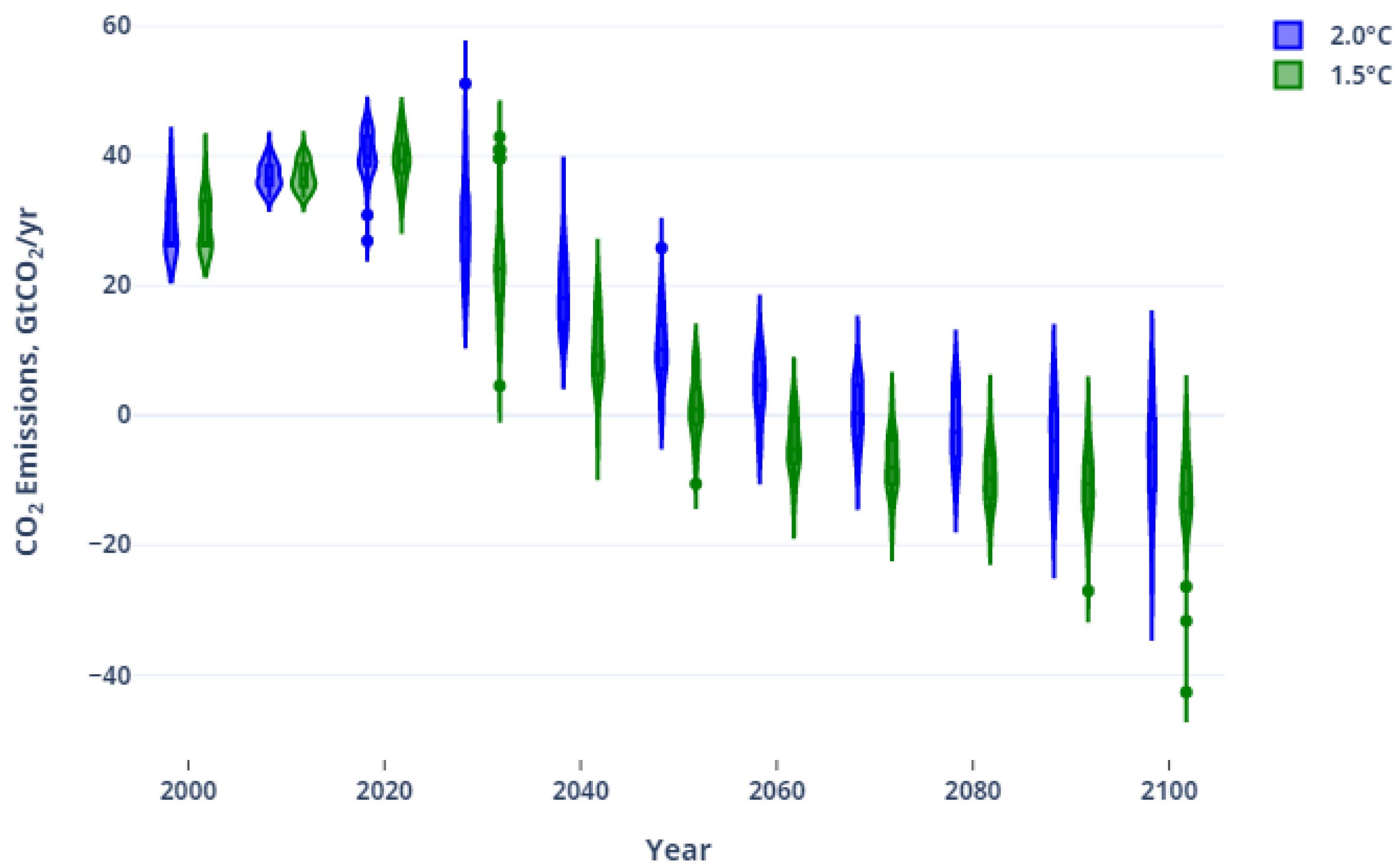
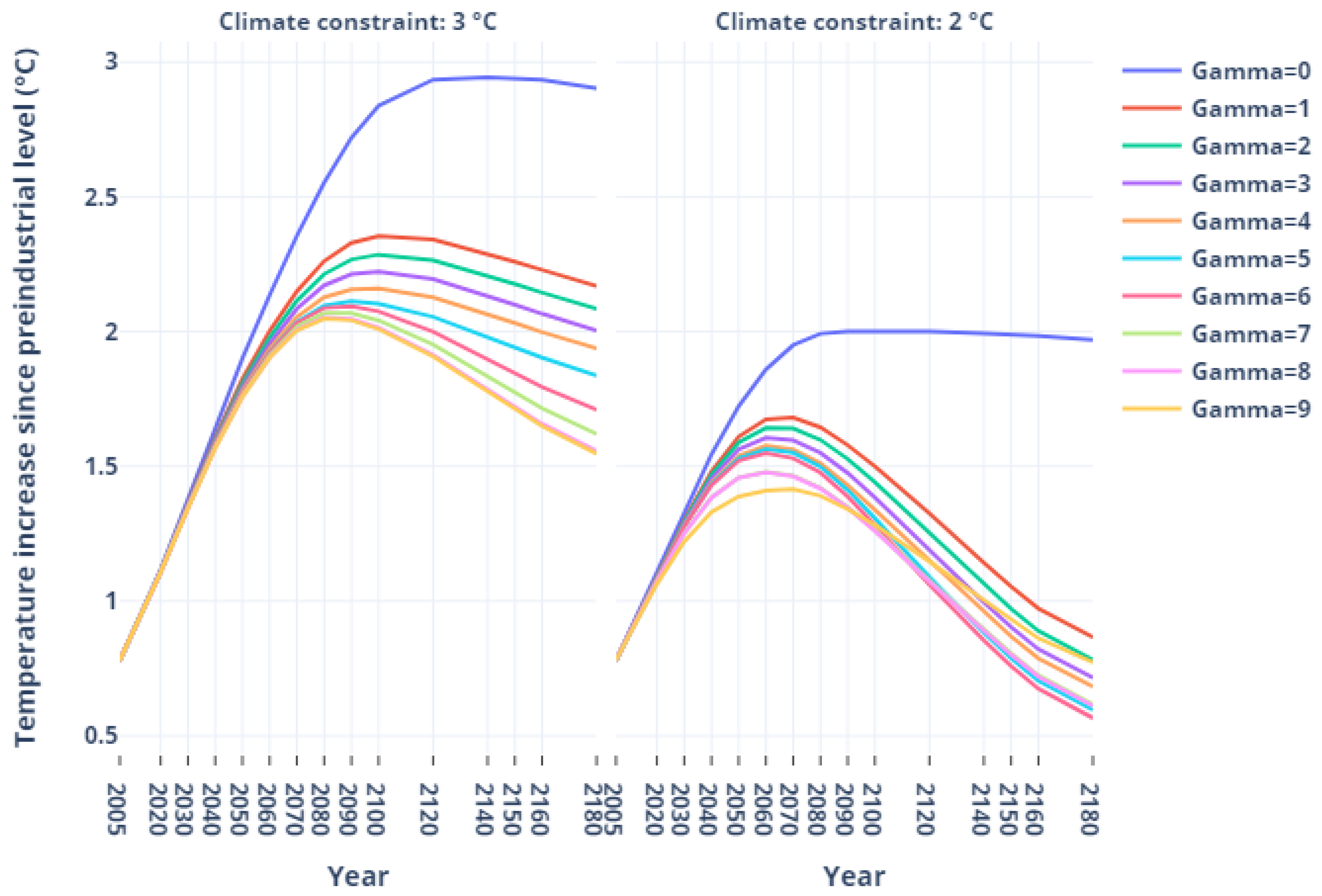
4.1. Temperature and Emission Trajectories

Figure 3 gives the temperature trajectories obtained with the nominal values of the climate parameters, when the trajectory with deviated parameters has to respect the 2 °C or 3 °C limit. They can be viewed as hedging trajectories: they should be followed in order to comply with the temperature constraint even in presence of parameter uncertainty. An increase in the uncertainty budget corresponds to an increase in the protection level.
Uncertainty has a significant impact on the temperature trajectories, even for the uncertainty budget’s low values. In order to ensure that the temperature does not exceed 2 °C (respectively, 3 °C), we should aim for a temperature increase ranged between 1.3 °C and 1.5 °C (resp., between 2 °C and 2.3 °C) with the nominal climate model in 2100. These new targets are consistent with the levels (1.5 °C and 2 °C) proposed by the Paris Agreement. Figure 3 reveals also that, to immunize against climate uncertainty with a 2 °C temperature limit, temperature peaks between 2060 and 2070 before decreasing rapidly. This notably impacts the energy transition pathways needed to comply with these temperature limits; see Section 4.3. On the other hand, with a 3 °C temperature limit, temperature peaks only by the end of the century and decreases more slowly afterwards.
The robust optimization approach also makes it possible to rank the parameters or group of parameters by sensitivity. Table 2 shows the order in which climate parameters deviate, characterizing a diminishing negative impact on the temperature constraint. Since the robust counterpart of the nominal problem maximizes the temperature deviation for a given emission profile, increasing the uncertainty budget consists in finding parameters with the worst effect on the solution within the set of remaining (undeviated) parameters.
The first deviating parameter is the climate sensitivity ( C S ). This can be explained by (i) its wide uncertainty range compared to the ones of the other parameters and (ii) the fact that it is a central parameter of the climate module. This is consistent with other studies analyzing climate response sensitivity to derive 2 °C-compliant mitigation pathways [45,75,76]. More interestingly, after the climate sensitivity, the most critical parameters are the ones of the carbon cycle ( ϕ a u and ϕ u a ). The terrestrial carbon dynamics is indeed of primary importance to assess the impact of anthropogenic GHG emissions, as it influences directly the atmospheric carbon concentration, and hence the radiative forcing and the temperature. This strengthens the importance of relying on appropriate uncertainty ranges for the climate parameters; see Appendix C. This also pleads for the necessity to pay more attention in IAMs to the intricacies of the carbon cycle, including feedbacks and non-linearities. Although climate sensitivity and the carbon cycle appear as primary factors, second-order parameters are ranked very differently. This may be (at least partially) explained by the mitigation dynamics in the two climate scenarios: in the 2 °C case, mitigation pathways must be implemented earlier (see the next figure) such that the climate dynamics does not have the same overall impact.
Figure 4 displays CO 2 emission trajectories for the nominal scenarios and emission ranges in the robust scenarios.
In the nominal trajectories, emissions peak by the middle of the century in the 3 °C case, and decreases rapidly afterwards. Whereas in the 2 °C case, emissions must decrease rapidly from 2020 on. Looking at the range of robust trajectories (shaded areas), it roughly expands over time in the 3 °C case to reach a maximum size by 2080; whereas in the 2 °C case, it reaches its maximum size earlier (2040). These dynamics are necessary to respect the different temperature profiles and implies contrasted energy transition pathways (both in terms of transition timing and energy portfolios); see Section 4.3. Note also the presence of negative emissions due to specific energy systems (see again Section 4.3).

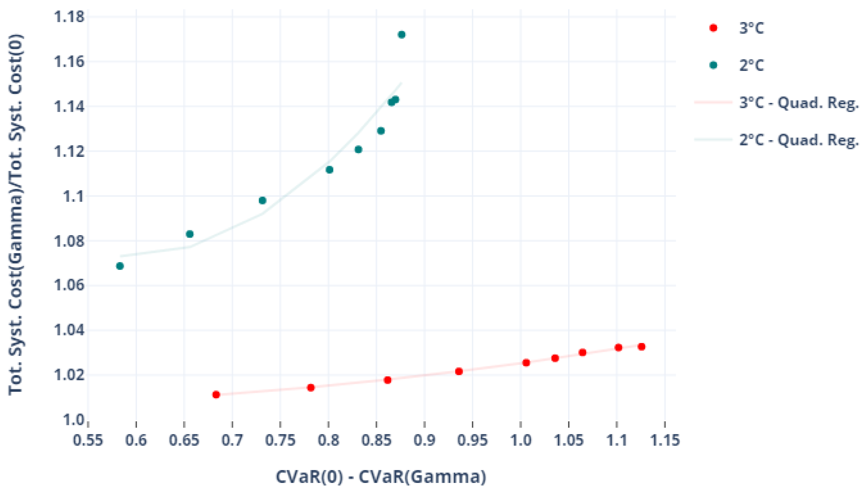
4.2. Robustness Cost

Let us now assess how using a robust model rather than a deterministic one impacts the total energy system cost (TIAM-World’s objective function), which yields the robustness cost. More precisely, we assess the trade-off between optimality (low system cost) and robustness (high protection level) by plotting in Figure 5 the cost increases with the ‘insurance/protection’ level. It has been constructed through Monte-Carlo simulations, using the emission trajectories obtained for each value of Γ with a temperature constraint ( T l i m = 2 °C or 3 °C) (see Figure A5). The climate model parameters considered are uniformly distributed on the previously defined uncertainty ranges. We are then able to derive the VaR and the CVaR95 for the temperature deviation in 2100 for both constraints. Intuitively, we expect the CVaR95 to be lower when the degree of conservatism (and the economic cost) of the solution is increased. Therefore, the incremental cost of insurance could be expressed as the additional system cost per unit of temperature insured:
f ( x * , Γ i ) f ( x * , Γ 0 ) C V a R 95 ( Γ 0 ) C V a R 95 ( Γ i )
On the abscissa, we report the temperature deviation against which we ‘insure’ ourselves using the optimal robust pathway: x ( T l i m , 2100 , Γ ) = C V a R ( T l i m , 2100 , 0 ) C V a R ( T l i m , 2100 , Γ ) ; see Appendix E for plots of the distributions obtained. The ordinate represents the objective function (the total system cost or TSC) obtained for different value of the protection level normalized by the deterministic case objective function.
Figure 5 depicts how the world energy system and its emissions adapt to increasing protection levels with respect to a reference temperature target. It reads as the cost increase to support in order to ‘buy’ a certain amount of protection level given the uncertain response of the climate system: insuring against the risk that the 5%-CVaR of the average temperature increase will not be higher than x x (or reducing it by x x compared to the nominal case).
This function aggregates two elements, namely: (i) the evolution of the total energy system cost with an increasing uncertainty budget (increasing protection level); and (ii) the CVaR-computed protection level associated to the change in global GHG emissions trajectory. Both are by construction concave functions of the uncertainty budget Γ . Indeed, the robust hedging strategies are driven by a worst-case logic, which implies that the incremental cost of increasing the uncertainty budget is necessarily diminishing. The same principle applies to GHG emissions. Interestingly, the process of composing these two functions yields a convex-shaped function. This implies that although both the temperature-expressed protection level and the incremental cost are concave shaped, the incremental cost still grows faster than the temperature hedge acquired.
Overall, this plot is comparable to a ‘standard’ temperature-based marginal abatement cost curve, except that it embeds a consistent risk perspective which combines robust optimization and a simple CVaR metrics for the output GHG emissions pathways. Comparing the two series for different climate constraints, it appears naturally that costs of protection are higher for the 2 °C series, and also more convex, yielding higher marginal costs.

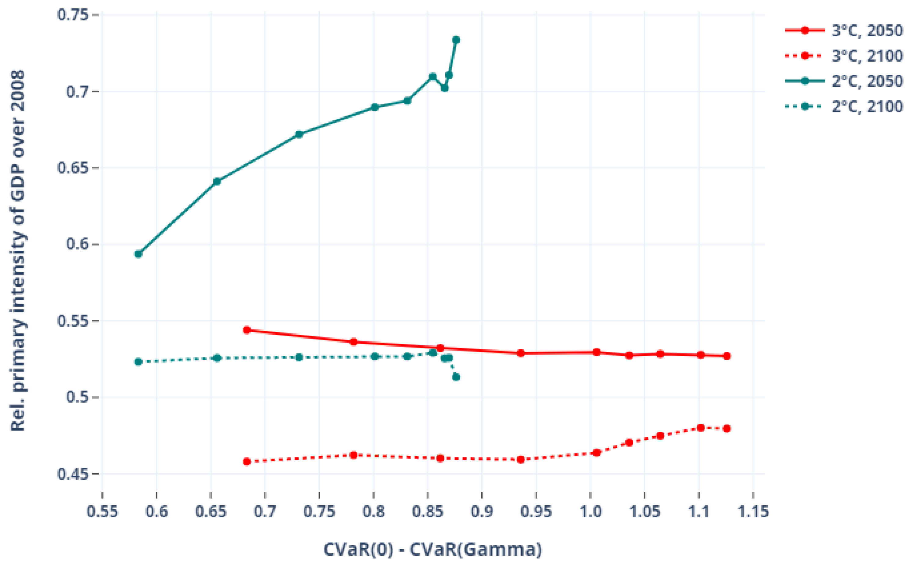
4.3. Robust Energy Transition Pathways

Increasing the required protection level for a given nominal temperature target implies an adaptation of the energy system towards lower GHG emission levels. This section describes salient elements of these robust energy transition pathways.

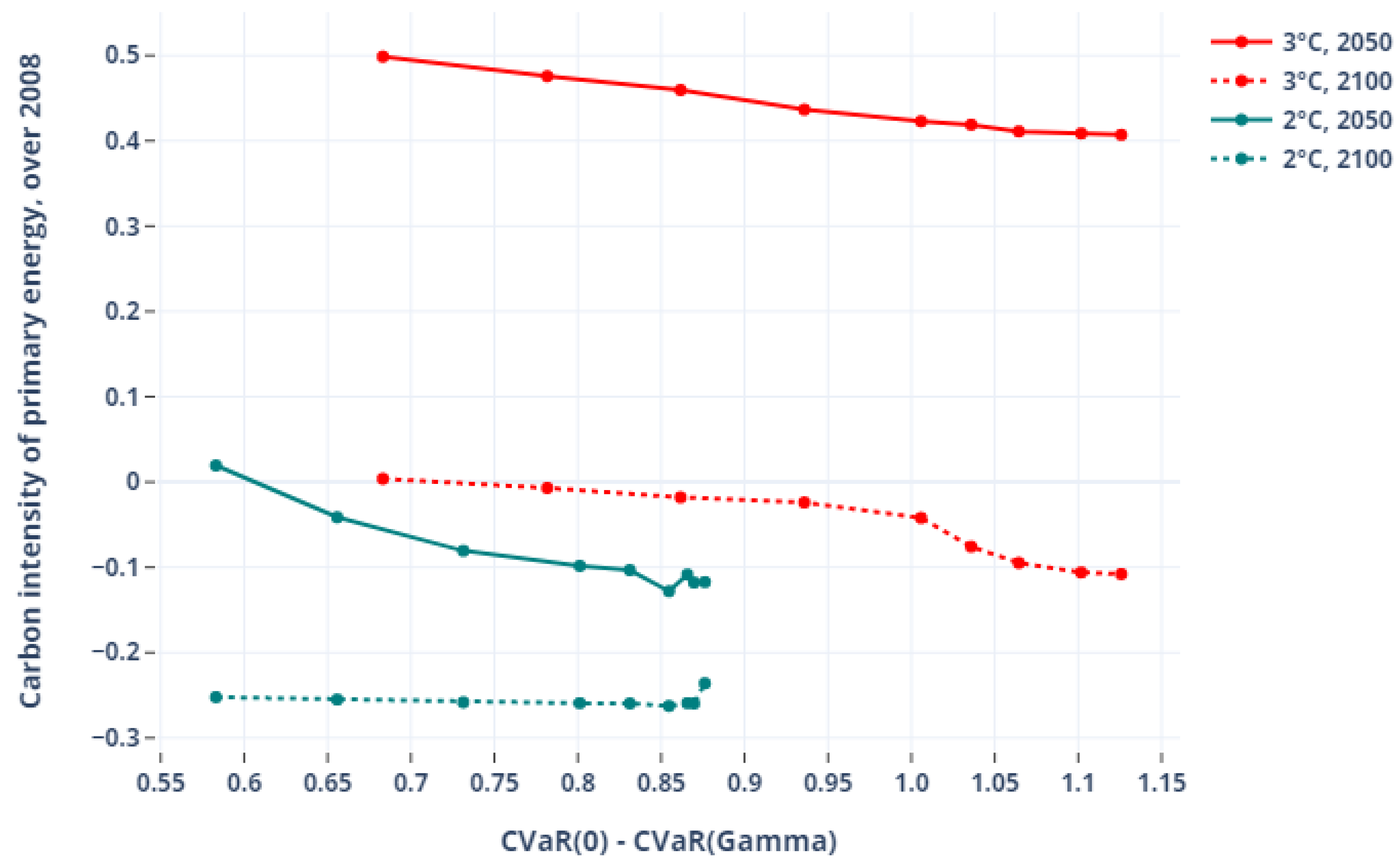
4.3.1. Robust Decarbonization Challenges: A Mesoscopic View

Figure 6 plots the world primary energy intensity of GDP, in 2050 and 2100, for the 3 °C and 2 °C targets (2050: plain lines, 2100: dashed lines; 3 °C: blue dot markers, 2 °C: red square markers) as a function of the protection level and 2008 normalized ( P E I r a t i o = P r i m a r y _ E n e r g y ( Y r ) G D P ( Y r ) × G D P ( 2008 ) P r i m a r y _ E n e r g y ( 2008 ) ). Primary energy consumptions are computed as the sum of coal, crude oil, natural gas, enriched uranium, biomass, solar, and wind energy consumed in the whole energy system. With the same convention, Figure 7 plots the evolution of the carbon intensity of primary energy with the protection level ( C I r a t i o = C O 2 ( Y r ) P r i m a r y _ E n e r g y ( Y r ) × P r i m a r y _ E n e r g y ( 2008 ) C O 2 ( 2008 ) ).
The evolution of these two intensities reflects very different strategies for the 3 °C and 2 C constraints. Hedging against climate uncertainty at the 3 °C level shows a balanced use of energy efficiency and decarbonization of primary energy in 2050; the two indicators show comparable reduction levels (more or less 50%) compared to the 2008 reference. In 2100, the 3 °C scenario hedges with a stronger reduction of carbon intensity, at the expense of primary energy intensity: carbon intensity drops with hedging (−50% to −60%) while energy intensity remains quite flat (−45% to −47%). This is especially true for higher protection levels for which CCS massively penetrates the decarbonization mix (see below). This yields negative carbon intensities, indicating negative net emissions. CCS-ready technologies being less efficient than their non-CCS equivalents, the primary energy requirements increase (moderately) with hedging.
At the 2 °C level, the trade-off between energy intensity and carbon intensity is anticipated as early as 2050. With increased protection levels, the fall of primary energy intensity of GDP is smaller (from −40% to −30% compared to 2008), while the carbon intensity of GDP is reduced by an additional 10% going to negative values and hence negative net emissions. In 2050, a slight instability is visible for the highest protection levels. It is due to the fact that the parameter that deviates when the instability occurs is the adjustment speed for atmospheric temperature, impacting slightly the dynamic of temperature evolution and leading to larger emission reductions in the short term. By 2100, protection strategies have reached a status-quo situation with the amount of climatic uncertainty. Both the primary energy intensity and the carbon intensity have become insensitive to the protection level. The maximum abatement potential is thus reached (reflecting the model limits).
Overall, between the two climate scenarios, comparable strategies are chosen (trade-off between energy intensity and carbon intensity, with the necessity to spend more energy to store carbon) but with a large difference in timing. This result is consistent with the temperature observation and CO 2 emissions paths, which show that protection at the 3 °C level is an endpoint issue (mitigation occurs in the second half of the century), while protection at the 2 °C level is a midpoint question (mitigation is extremely strong by 2050, but final states—2100—show less variability). This raises the question of the economy’s decarbonization speed, and how to reach, e.g., COP21 compliant objectives.

4.3.2. Robust Energy Portfolios

Although the previous results show an aggregate picture of reduction and mitigation strategies in an uncertain climate context, further desegregating the primary energy consumption level (see Figure 8) offers additional insights.
Both the 3 °C and the 2 °C scenario groups show similarities. Naturally, increasing protection and/or imposing a more stringent climate objective tend to reduce the use of the most carbonized energy sources (coal, gas) in favour of renewable energy sources (solar, wind, biomass) (see also Table 3).
As primary energy sources with high carbon contents, gas and coal uses are highly elastic to the protection level. Gas use decreases between 13% and 20% in 2050 and between 32% and 75% in 2100 in the 3 °C scenarios (always compared to the deterministic case in the same target scenario group). At the same time, coal use is diminished by 22% to 36% in 2050 and 53% to 65% in 2100. The scenarios for the 2 °C target show a comparable albeit amplified tendency: both energy source uses diminish by 75% to 90% in 2050 and 2100. At the same time, the use of renewable energy raises in any case, up to 200% in 2050 for the 2 °C scenarios. Although for the 3 °C scenarios, renewable use is tripled between 2050 and 2100. In the renewable group, biomass plays a prominent role since its use coupled with CCS is critical for decarbonization (as it generates negative emissions).
Nuclear is an option for decarbonizing the economy, and more precisely a power intensive economy which relies more on carbon-neutral sources. The use of uranium gradually increases by 2100 in the 3 °C scenarios, and much faster in the 2 °C scenarios (up to 2050) before stabilizing. Lastly, oil plays a particular role: while the use of other fossil energy decreases, the amount of crude oil consumed in the primary energy mix is rather stable across scenarios and protection levels. This tendency to maintain the use of oil products is to be related to the difficulty of reducing transport emissions (high abatement costs) combined with the large availability of low-carbon alternatives in other sectors (nuclear, CCS).

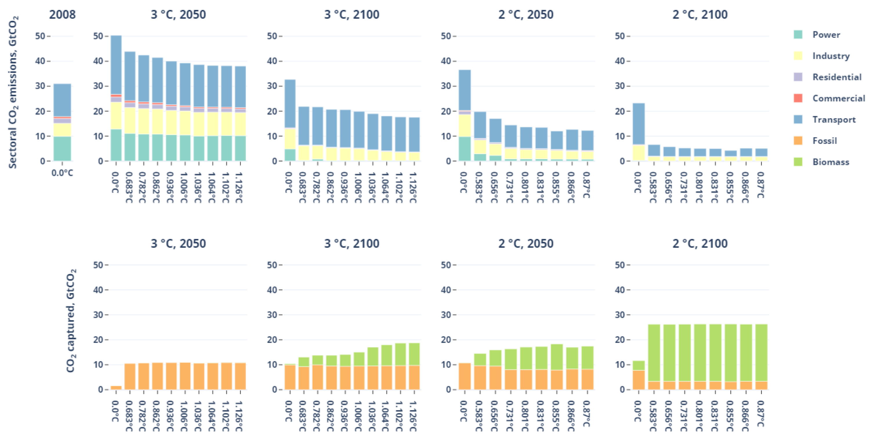
4.3.3. A Sectoral View: The ‘Backstop’ Negative Emissions Pathways against Low-Elastic Transport

Figure 9 presents the role of the various sectors in the decarbonization process.
Regardless of the scenario, transport remains the main CO 2 emitter worldwide. In the 3 °C case, all emissions peak around 2040 before falling—with the exception of the transport sector—alternative technologies penetrate the mix. Electricity and industry are the main contributors to abatement, essentially between 2050 and 2100. In 2100, transport emissions represent between 60% and 90% of the end-use emissions; they are rather stable in absolute terms, so that technology improvements (efficiency, low-carbon fuels) compensate for the demand growth. Although CCS is deployed by 2050 as a hedge for about 10 Gt/yr, transport emissions in the second half of the century are compensated by credits from CCS captured from biomass (negative emissions).
The 2 °C case differs in three ways. First, the need to reduce emissions further to remain compliant with a 2 °C target with uncertainty forces to reduce emissions from the power and industry sectors much faster (by 2050). Second, even transport emissions go down sharply to obtain to a 1.5 °C average elevation level. At this timescale, only transport and industry have some residual emissions. Third, the additional use of CCS from biomass fuelled power plants is not only incremental but also comes as a substitute for fossil CCS pathways. The importance of bioCCS in this picture reveals the importance of estimating biomass potentials and assessing relevant sensitivity analysis on the subject.
The clear-cut arbitrage strategy between biomass-CCS and transport emissions can be explained at the technology level, see Figure 10.
The analysis of the energy mix for transport shows a strong reliance on fossil-based fuels, which represent a large part of the mix except in the longer term for the 2 °C target. In that case, transport fuels have become almost carbon free with a strong reliance on hydrogen. Since transport is a sector with high abatement costs [77], it is only when the protection level is high that the oil trajectory is impacted. The vehicle fleet is progressively electrified, with diesel and gasoline losing market share with time and uncertainty. Electric vehicles appear as a relevant way to mitigate the risk induced by climate uncertainty. In addition, in energy terms, the moderate penetration of electricity as a transportation fuel minimizes a wider reality: while electricity can represent up to 30% of the energy used in transport, the relative efficiency of electric vehicles compared to conventional ones (2 to 2.5 more efficient) implies that, in 2050, more than 50% of the total world mobility is actually electromobility. Yet, the commercial transportation fleet sticks with diesel trucks, leading to a stable diesel consumption.
In the power sector, the protection level increase leads to an early use of CCS, as early as 2030 in most cases (see also Figure 9). The nuclear and the CCS trajectories under uncertainty have large consequences in terms of policy decision. For example, given the current state of R&D on CCS (with various projects shut down this last decade), this result suggests that we may want to reconsider the current R&D budget allocation. The importance of nuclear in the energy mix is also at odds with some nation’s policies, such as Germany. Indeed, they decided some years ago to close all the nuclear plants in a near future (unlike Japan, where nuclear plants are planned to restart in the near future). Negative emission possibility is also something quite abstract and subject to much uncertainty, as the first commercial-scale biomass-fuelled power plant with CCS has yet to be built.

5. Conclusions

Climate modelling is hampered by a considerable amount of uncertainty because of the lack of knowledge of the climate system. As it significantly impacts climate policy making, the need for tools to evaluate robust transition pathways is more and more urgent. In this paper, we present a robust approach to handling climate uncertainty in Integrated Assessment Models (IAMs).
We find that the climate module’s most sensitive parameter is the climate sensitivity. This is consistent with the existing literature on the subject. Climate sensitivity is the most studied parameters and that its value estimations are numerous. Hence, the determination of the climate sensitivity uncertainty range is quite straightforward. Another important point is that this range relies on a large information set unlike the other parameters, for which data are scarce. Indeed, information on the carbon cycle parameters is scarce (few studies in the IAMs climate module literature) and yet the global climate system behaviour is very sensitive to them. Moreover, climate parameters impact diversely the timing of the adaptation: the radiative forcing sensitivity multiplies directly the CO 2 concentration, hence even a small variation of this parameter leads to a strong impact on the CO 2 abatement timing. We then believe that a stronger focus should be put on the other climate model parameters.
To ensure that we comply with a 3 °C constraint, the temperature trajectories we should aim at with the nominal parameters should not exceed 2.4 °C, leading to zero net carbon emissions at the end of the century. With a 2 °C constraint, we should aim at 1.6 °C with negative carbon emissions as soon as 2050. If the insurance cost is quite reasonable for the higher constraint (from 1.5% to 4% of the system total discounted cost), it is less the case with a 2 °C objective. In the latter situation, the total discounted system cost increases by 7% when the protection level is low and up to 14% when it is high. This is because to comply with a stringent target, sectors with high abatement costs have to participate in the global reduction effort. For example, transport is little impacted by the 3 °C target (but as the protection level increases, the vehicle fleet is slightly modified), whereas the introduction of uncertainty leads to major fuel consumption changes for the 2 °C constraint.
Abatement strategies are quite different between the two temperature targets. For the 3 °C target, both the carbon intensity and the primary energy intensity of the economy decrease with the protection level whereas for the 2 °C target, the energy intensity increases and the carbon intensity decreases. This more stringent goal is reached by investing massively in carbon removal technologies such as bioenergy with carbon capture and storage (BECCS) which have yields much lower than traditional fossil fuelled technologies. Another interesting fact of the 2 °C hedging trajectories is the drastic increase in the nuclear electricity production. The massive use of nuclear or carbon removal technology is highly uncertain as BECCS is a very expensive technology that is not competitive in the absence of a high CO 2 price, while the development of the nuclear industry could be hampered by social acceptance issues. The 1.5 °C objective mentioned during the COP21 is obviously very ambitious and reaching it would necessitate strong political and societal ambitions and actions (much stronger than the ones decided during the COP21).
By taking a robust approach to study ways of complying with ambitious climate targets, we were able to bring to light hedging technological trajectories without excessive computational issues. The method presented being quite generic, it could be interesting to perform similar exercises with other IAMs. It would help strengthen the knowledge on technological transition pathways with uncertainty and would allow a better understanding and awareness of the costs of the risks linked to our partial knowledge of the climate system.

Author Contributions

C.N.: conceptualization, data curation, investigation, methodology, validation, visualisation, Writing—original draft, Writing—review & editing, S.T.-M.: conceptualization, investigation, methodology, validation, visualisation, Writing—original draft, Writing—review & editing, E.D.: methodology, validation, Writing—review & editing and O.B.: methodology, Writing—review & editing. All authors have read and agreed to the published version of the manuscript.

Funding

Olivier Bahn and Erick Delage both acknowledge the financial support from the Natural Sciences and Engineering Research Council of Canada (respectively RGPIN-2016-04214 and RGPIN-2016-05208).

Institutional Review Board Statement

Not applicable.

Informed Consent Statement

Not applicable.

Data Availability Statement

Not applicable.

Acknowledgments

The authors thank Alain Ayong le Kama and three anonymous reviewers for their insightful comments.

Conflicts of Interest

Not applicable.

Abbreviations

The following abbreviations are used in this manuscript:
BECCSBioenergy with carbon capture and storage
CCSCarbon capture and storage
EMICEarth System Models of Intermediate Complexity
GHGGreenhouse gas
IAIntegrated Assessment
IAMIntegrated Assessment Model
IPCCIntergovernmental Panel on Climate Change
RCPRepresentative Concentration Pathway
RORobust optimization
SCMSimple Climate Model
TSCTotal System Cost

Appendix A. Model Overview

The TIMES Integrated Assessment Model (TIAM-World) is a detailed, global, multi-region technology-rich model of the energy/emission system of the world. It is based on the The Integrated MARKAL-EFOM System (TIMES) economic paradigm, which computes an inter-temporal dynamic partial equilibrium on energy and emission markets based on the maximization of total surplus (A complete description of the TIMES equations appears in www.etsap.org/documentation). TIAM-World is described in [11,47]. It is used in many international and European projects (for recent applications see: [43,72]).
The multi-region partial equilibrium model of the energy systems of the entire World is divided in 16 regions. Regions are linked by trade variables of the main energy forms (coal, oil, gas) and of emission permits (see Figure A1). TIAM’s planning horizon extends from 2000 to 2100, divided into periods of varying lengths.
Figure A1. TIAM reference energy system.
Energies 14 08595 g0a1
In TIMES, an intertemporal dynamic partial equilibrium on energy markets is computed, where demands for energy services are exogenously specified (only in the reference case), and are sensitive to price changes in alternate scenarios via a set of own-price elasticities at each period. Although TIMES does not encompass all macroeconomic variables beyond the energy sector, accounting for price elasticity of demands captures a major element of feedback effects between the energy system and the economy. Thus, the equilibrium is driven by the maximization (via linear programming) of the discounted present value of total surplus, representing the sum of surplus of producers and consumers, which acts as a proxy for welfare in each region of the model (practically, the LP minimizes the negative of the surplus, which is then called the energy system cost).
The maximization is subject to many constraints, such as: supply bounds (in the form of supply curves) for the primary resources, technical constraints governing the use of each technology, balance constraints for all energy forms and emissions, timing of investment payments and other cash flows, and the satisfaction of a set of demands for energy services in all sectors of the economy.
The nominal formulation of the TIAM problem is a cost minimization and can be written as follows (with some simplifications):
min t c t T x t s . t . L t x t b t , x t R n , L t R m * n , ( technological constraints ) D t x t d t , x t R n , D t R d * n , ( demand constraints ) y t w t , with y t = A y t 1 + F x t , ( recursive climate constraints ) x t R n , y t R w , A R w * w , F R w * n
The objective function is the total cost of the system. It includes, among others: investment costs, operating costs of the various sectors, taxes, transportation costs between geographical zones. Technological constraints cover capacity limits, supply limits, yields, the allowed growth rates of the processes in the various sectors. Demand constraints include each zone’s energy service demands and climate constraints embrace limits on GHG emissions or stocks in the atmosphere or on temperature increase. These latter constraints belong to an endogenous climate module. Note that the CO 2 , CH 4 and N 2 O emissions related to the energy sector are explicitly represented by the energy technologies included in the model. The non-energy-related CO 2 , CH 4 and N 2 O emissions (landfills, manure, rice paddies, enteric fermentation, waste water, and land use) are also included in order to correctly represent the radiative forcing induced by them, but they are exogenously defined. Emissions from some Kyoto gases (CFCs, HFCs, and SF6) are not explicitly modelled, but a special radiative forcing term is added in the climate module.

Appendix B. TIAM-World Climate Module

The climate module used in TIAM-World for this work is an adapted version of the model developed by Nordhaus and Boyer [73]. Greenhouse gas concentration and temperature changes are calculated from linear recursive equations. We briefly present its characteristics here, a detailed description can be found in Loulou et al. [74].
The climate representation in TIAM-World is characterized by three steps. First, the GHGs emitted by anthropogenic activities accumulate in the atmosphere; exchanges with the upper and deep ocean layers occur then for CO 2 , while the dissipation of CH 4 and N 2 O is described with single atmospheric decay parameters.
The terrestrial carbon cycle of this climate module is depicted in Figure A2. Formally, the one-year-lagged dynamics of the three detailed greenhouse gases are the following:
M C O 2 , a M C O 2 , u M C O 2 , l t = Φ C O 2 M C O 2 , a M C O 2 , u M C O 2 , l t 1 + 1 0 0 E t C O 2 , M C H 4 , a M C H 4 , u t = Φ C H 4 M C H 4 , a M C H 4 , u t 1 + 1 0 E t C H 4 , M N 2 O , a M N 2 O , u t = Φ N 2 O M N 2 O , a M N 2 O , u t 1 + 1 0 E t N 2 O , Φ C O 2 = 1 φ a u φ u a 0 φ a u 1 φ u a φ u l φ l u 0 φ u l 1 φ l u , Φ C H 4 = φ C H 4 0 0 1 , Φ N 2 O = φ N 2 O 0 0 1 ,
where M t g , r is the mass of gas g in reservoir r in year t, E t g is the emission of gas g in year t (from the global energy model), φ r o , r i is the transfer coefficient for CO 2 from reservoir r o to reservoir r i , φ C H 4 and φ N 2 O are the decay rates of methane and nitrous oxide in the atmosphere, g G = C O 2 , C H 4 , N 2 O and r R = a = A t m o s p h e r e , u = U p p e r L a y e r , l = L o w e r L a y e r .
This set of equations defining the time profiles of atmospheric GHGs is then used to compute the radiative forcing. It is common [78] to consider that forcings are additive, so that:
Δ F t = g G Δ F t g + E x f t ,
where Δ F t g is the forcing of gas g in period t and E x f t corresponds to an exogenous assumption of forcing for all gases other than carbon dioxide, methane, and nitrous oxide. The current knowledge on radiative forcing suggests that none of these terms is linear in the atmospheric stock of gas; the linearization used here is proposed by [74]:
Δ F t C O 2 = γ A C O 2 + γ B C O 2 M t C O 2 , a , Δ F t C H 4 = A C H 4 + B C H 4 M t C H 4 , a , Δ F t N 2 O = A N 2 O + B N 2 O M t N 2 O , a ,
where γ is the radiative forcing sensitivity to atmospheric CO 2 doubling, and A’s and B’s are constant depending on pre-industrial concentration levels and linearization intervals. Finally, temperature elevation profiles are computed based on the following equations:
Δ T u p Δ T l o t = S Δ T u p Δ T l o t 1 + σ 1 0 Δ F t , S = 1 σ 1 γ C S + σ 2 σ 1 σ 2 σ 3 1 σ 3 .
where Δ T u p is the variation of the atmospheric temperature, Δ T l o the variation of the ocean temperature, C S represents the climate sensitivity, i.e., the change in equilibrium atmospheric temperature due to a doubling of GHG concentration; σ 1 and σ 3 are the adjustment speeds for, respectively, atmospheric and oceanic temperature (lags, in y e a r 1 ); σ 2 is a heat loss coefficient from the atmosphere to the deep ocean.
Figure A2. TIAM climate module.
Energies 14 08595 g0a2

Appendix C. Estimation of Lower/Upper Bounds for Climate Parameters

Overall, and in the course of this estimation exercise, we may classify the climate parameters at stake in this study into three groups. First, one group contains the parameters for the carbon cycle. The terrestrial carbon cycle itself is a rather large field of study in geophysics (see, e.g., [59,60]; for a multi-model approach). One can also find sensitivity analysis on the carbon cycle in IAM-based research [62,64], or are least clues on how uncertain these parameters are [14]. One way of assessing the behaviour of carbon cycle models is to perform the so-called ‘doubling experiment’, where the evolution of an atmospheric CO 2 doubling-concentration pulse in year 0 is followed across the various carbon sinks for the next 100–400 years. Existing multi-models experiments [48,60] point out large response spectra; Ref. [48] additionally shows that simple carbon models (few boxes, simple linear recursive dynamics) such as DICE end up in the low range of possible outcomes: they have, compared to the rest, relatively optimistic carbon cycles. Such an experiment seems to be a good starting point to calibrate a carbon cycle. However, the uncertainty it translates covers both parametric and structural uncertainty. For example, Ref. [48] argues that the PAGE model behaves very differently from the rest of the test population because it includes feedbacks on the carbon cycle. This limitation—carbon cycle models have different structures, hence different parameters—makes it difficult to adopt such a calibration procedure. Therefore, we adopt a calibration procedure similar to that of [66], but for the four IPCC-RCP emissions scenarios ran under the multi-ensemble simulation mode of MAGICC6 [49]. To this purpose:
  • The nominal values of the parameters in the climate module in TIAM-World was left as described in [74];
  • The upper bound of the inter-boxes transfer coefficients were estimated to become close to the 83rd percentile of the MAGICC6 inter-model simulations for the four RCP scenarios. This is done by changing the parameters by identical relative amounts, and computing a simple distance measure (the sum of squares of annual relative distances between the TIAM-climate simulation and the MAGICC6-RCP benchmark).
The result of this experiment is shown in Figure A3. The blue lines and shade represent, in each subgraph, the average, 95% and 90% confidence intervals produced by MAGICC6. The black plain and dotted show the average and 95% confidence intervals obtained with the TIAM-World climate module.
Figure A3. TIAM-World climate module: Uncertainty in the carbon cycle against MAGICC6 ranges for the four RCP scenarios.
Energies 14 08595 g0a3
These variations allow to capture only a minor part of the carbon cycle model variations described by [48] or [60]. Ref. [62] shows that the variations in climate change benefits from a set of IAMs due to the carbon cycle are lower than the MAGICC6 ranges, which seems to indeed indicate that simple carbon cycles do not capture all the ‘volatility’ of outcomes.
A second set of parameters includes the forcing and climate sensitivities, which are likely to be the most well-documented parameters in the climate literature. They traduce the global equilibrium surface forcing and warming after a doubling of atmospheric CO 2 concentration; any climate models includes these parameters. The importance of the equilibrium radiative forcing is widely acknowledged [67]; multi-models comparisons and simulations are also frequent [68]. If issues such as climate feedbacks arise in the estimation of forcing [69], available comparisons indicate plausible range for the forcing parameters (using doubling or quadrupling experiments), with the last IPCC report (AR5-WG1, [70]) providing a central value of 3.7 with a +/− 0.8 99% confidence interval. This estimation is consistent with [71], and is retained for this study. As for the climate sensitivity, the initial value of the TIAM-World calibration corresponds to the [65] synthesize plausible sensitivity ranges for the climate sensitivity for different lines of evidence, and demonstrate how critical it is if the policy objective is to prevent damages caused by certain levels of warming. The IPCC most likely value and upper bound are 3 °C and 4.5 °C, respectively, which is consistent with other papers, such as [50]. Ref. [64] makes a different choice, and end up with a range (upper bound of 8 °C) closer to what [65] refer to as ‘expert elicitation’. Combining different lines of evidence, these authors obtain a range close to the one of IPCC, which we will retain as a basis. Compared to existing literature on IAM-SCM sensitivity analysis in [64], these ranges are high for forcing and low for the climate sensitivity.
Finally, the rest of the parameters, traducing the temperature dynamics, are part of a third group constituted of apparently less studied parameters. There seems to be considerably less available work on these. By default, we proceed as [64], and apply a 10% variation to the annual heat transfer coefficients. The range of temperature responses of TIAM-World are compared against MAGICC6 for the 4 RCPs scenarios, accounting for the uncertainty of all parameters. The results are presented in Figure A4 (it reads as Figure A3).
Figure A4. TIAM-World climate module: Uncertainty in the global mean temperature against MAGICC6 ranges for the four RCP scenarios.
Energies 14 08595 g0a4
The final nominal values and ranges for the climate parameters are presented in Table A1 along with the values kept in [64] for comparison purposes.
Table A1. Nominal values for climate parameters and comparison with [64].
ParameterDescriptionNominal Value (This Paper)Lower/ Upper Bound (This Paper)Nominal Value (Bulter)Lower/ Upper Bound (Butler)
ϕ a u Atmosphere to upper layer carbon transfer coefficient (annual)0.0460.043930.1892880.223288
ϕ u a Upper layer to atmosphere carbon transfer coefficient (annual)0.04530.04733850.097213derived
ϕ u l Upper to lower layer carbon transfer coefficient (annual)0.01460.0139430.050.025
ϕ l u Lower to upper layer carbon transfer coefficient (annual)0.000530.000553850.003119derived
γ Radiative forcing from doubling of CO 2 3.74.53.83.9
C S Climate sensitivity from doubling of CO 2 2.94.538
σ 1 Adjustment speed of atmospheric temperature0.0240.02640.220.24
σ 2 Heat loss from atmosphere to deep ocean0.440.3960.30.27
σ 3 Heat gain by deep ocean0.0020.00180.050.045

Appendix D. Implementation Details for the Worst-Case Oracle in TIAM-World Model

For simplicity of exposure, we describe the procedure for solving Problem (11) when the respective worst-case extreme value (between minimum and maximum) for each parameter can be identified a-priori (either analytically or using common sense). Following the information presented in Table 1, we can describe the uncertainty as follows:
ψ a u : = ψ ¯ a u ψ ^ a u z 1 ψ u a : = ψ ¯ u a + ψ ^ u a z 2 ψ u l : = ψ ¯ u l ψ ^ u l z 3 ψ l u : = ψ ¯ l u + ψ ^ l u z 4 γ : = γ ¯ + γ ^ z 5 ( 1 / C s ) : = ( 1 / C ¯ s ) ( C ^ s / ( C ¯ s 2 + C ¯ s C ^ s ) ) z 6 σ 1 : = σ ¯ 1 + σ ^ 1 z 7 σ 2 : = σ ¯ 2 + σ ^ 2 z 8 σ 3 : = σ ¯ 3 + σ ^ 3 z 9 ,
where the bar annotated parameter refers to the nominal value and the hat annotated parameter refers to the magnitude of the perturbation needed to obtain to the chosen extreme value. We also modelled the perturbation on the term 1 / C s using an additive formulation, namely:
1 / C s : = 1 / C ¯ s if z 6 = 1 1 / ( C ¯ s + C ^ s ) otherwise .
Based on the definitions of A and F, one should notice that these two matrices are not linear functions of the uncertainty z 1 , z 2 ,..., z 9 . This can be remedied by replacing the non-linearities with additional binary variables. In particular, when studying the effect of z on each term of A, one might realize that the following expressions come into play:
γ ψ a u = γ ¯ ψ ¯ a u γ ¯ ψ ^ a u z 1 + ψ ¯ a u γ ^ z 5 γ ^ ψ ^ a u z 1 z 5 γ ψ u a = γ ¯ ψ ¯ u a + γ ¯ ψ ^ u a z 2 + ψ ¯ u a γ ^ z 5 + γ ^ ψ ^ u a z 2 z 5 σ 1 γ ψ a u = σ ¯ 1 γ ¯ ψ ¯ a u σ ¯ 1 γ ¯ ψ ^ a u z 1 + σ ¯ 1 γ ^ ψ ¯ a u z 5 + σ ^ 1 γ ¯ ψ ¯ a u z 7 σ ¯ 1 γ ^ ψ ^ a u z 1 z 5 σ ^ 1 γ ¯ ψ ^ a u z 1 z 7 + σ ^ 1 γ ^ ψ ¯ a u z 5 z 7 + σ ^ 1 γ ^ ψ ^ a u z 1 z 5 z 7 σ 1 γ ψ u a = σ ¯ 1 γ ¯ ψ ¯ u a + σ ¯ 1 γ ¯ ψ ^ u a z 2 + σ ¯ 1 γ ^ ψ ¯ u a z 5 + σ ^ 1 γ ¯ ψ ¯ u a z 7 + σ ¯ 1 γ ^ ψ ^ u a z 2 z 5 + σ ^ 1 γ ¯ ψ ^ u a z 2 z 7 + σ ^ 1 γ ^ ψ ¯ u a z 5 z 7 + σ ^ 1 γ ^ ψ ^ u a z 2 z 5 z 7 σ 1 γ / C s = σ ¯ 1 γ ¯ θ ¯ + σ ¯ 1 γ ^ θ ¯ z 5 σ ¯ 1 γ ¯ θ ^ z 6 + σ ^ 1 γ ¯ θ ¯ z 7 σ ¯ 1 γ ^ θ ^ z 5 z 6 + σ ^ 1 γ ^ θ ¯ z 5 z 7 σ ^ 1 γ ^ θ ¯ z 6 z 7 σ ^ 1 γ ^ θ ^ z 5 z 6 z 7 σ 1 σ 2 = σ ¯ 1 σ ¯ 1 + σ ^ 1 σ ¯ 1 z 7 + σ ¯ σ ^ 2 z 8 + σ ¯ 1 σ ¯ 2 z 7 z 8 ,
where θ ¯ : = 1 / C ¯ s and θ ^ : = C ^ s / ( C ¯ s 2 + C ¯ s C ^ s ) . By making the replacement v 0 j k : = z j z k and v i j k : = z i z j z k , one would instead obtain the following set of linear representations:
γ ψ a u = γ ¯ ψ ¯ a u γ ¯ ψ ^ a u z 1 + ψ ¯ a u γ ^ z 5 γ ^ ψ ^ a u v 015 γ ψ u a = γ ¯ ψ ¯ u a + γ ¯ ψ ^ u a z 2 + ψ ¯ u a γ ^ z 5 + γ ^ ψ ^ u a v 025 σ 1 γ ψ a u = σ ¯ 1 γ ¯ ψ ¯ a u σ ¯ 1 γ ¯ ψ ^ a u z 1 + σ ¯ 1 γ ^ ψ ¯ a u z 5 + σ ^ 1 γ ¯ ψ ¯ a u z 7 σ ¯ 1 γ ^ ψ ^ a u v 015 σ ^ 1 γ ¯ ψ ^ a u v 017 + σ ^ 1 γ ^ ψ ¯ a u v 057 + σ ^ 1 γ ^ ψ ^ a u v 157 σ 1 γ ψ u a = σ ¯ 1 γ ¯ ψ ¯ u a + σ ¯ 1 γ ¯ ψ ^ u a z 2 + σ ¯ 1 γ ^ ψ ¯ u a z 5 + σ ^ 1 γ ¯ ψ ¯ u a z 7 + σ ¯ 1 γ ^ ψ ^ u a v 025 + σ ^ 1 γ ¯ ψ ^ u a v 027 + σ ^ 1 γ ^ ψ ¯ u a v 057 + σ ^ 1 γ ^ ψ ^ u a v 257 σ 1 γ / C s = σ ¯ 1 γ ¯ θ ¯ + σ ¯ 1 γ ^ θ ¯ z 5 σ ¯ 1 γ ¯ θ ^ z 6 + σ ^ 1 γ ¯ θ ¯ z 7 σ ¯ 1 γ ^ θ ^ v 056 + σ ^ 1 γ ^ θ ¯ v 057 σ ^ 1 γ ^ θ ¯ v 067 σ ^ 1 γ ^ θ ^ v 567 σ 1 σ 2 = σ ¯ 1 σ ¯ 1 + σ ^ 1 σ ¯ 1 z 7 + σ ¯ σ ^ 2 z 8 + σ ¯ 1 σ ¯ 2 v 078 ,
Hence, it becomes possible to represent U as:
U : = ( A , F ) w × w × w × n | z 0 = 1 , z { 0 , 1 } m , v { 0 , 1 } | S | i = 1 m z i Γ A = A ¯ + i = 1 m A ^ i z i + ( i , j , k ) S A ˜ i j k v i j k F = F ¯ + i = 1 m F ^ i z i + ( i , j , k ) S F ˜ i j k v i j k z i + z j + z k 2 v i j k ( 1 / 3 ) ( z i + z j + z k ) , ( i , j , k ) S
where
S : = ( 0 , 1 , 5 ) , ( 0 , 1 , 7 ) , ( 0 , 2 , 5 ) , ( 0 , 2 , 7 ) , ( 0 , 5 , 6 ) , ( 0 , 5 , 7 ) , ( 0 , 6 , 7 ) , ( 0 , 7 , 8 ) , ( 1 , 5 , 7 ) , ( 2 , 5 , 7 ) , ( 5 , 6 , 7 )
and where A ¯ + i A ^ i z i + ( i , j , k ) S A ˜ i j k v i j k and F ¯ + i F ^ i z i + ( i , j , k ) S F ˜ i j k v i j k are the respective linear matrix representations of A and F. Furthermore, the set of linear constraints that take the form:
z i + z j + z k 2 v i j k ( 1 / 3 ) ( z i + z j + z k ) ,
are simply a convenient way of representing the non-linear equality constraint v i j k = z i z j z k .
Having this representation for U in hand, Problem (11) can be described as:
max y , z , v y t w t s . t y τ + 1 = ( A ¯ + i A ^ i z i + ( i , j , k ) S A ˜ i j k v i j k ) y τ + ( F ¯ + i F ^ i z i + ( i , j , k ) S F ˜ i j k v i j k ) x τ , τ = 1 , , t i z i Γ z i + z j + z k 2 v i j k ( 1 / 3 ) ( z i + z j + z k ) , ( i , j , k ) S z { 0 , 1 } m , v { 0 , 1 } | S |
which is still a mixed integer non-linear program due to the cross-terms z i y τ and v i j k y τ .
In order to facilitate the resolution, we apply a second step of linearization by employing additional variables Z m × t and V | S | × t , such that Z i , τ : = z i y τ and V i j k , τ : = v i j k y τ . This leads to the following mixed integer linear program:
max y , z , v , Z , V y t s . t . y τ + 1 = A ¯ y τ + i A ^ i Z i , τ + ( i , j , k ) S A ˜ i j k V i j k , τ + F ¯ x τ + i F ^ i x τ z i + ( i , j , k ) S F ˜ i j k x τ v i j k F ¯ x τ + i F ^ i x τ z i + ( i , j , k ) S F ˜ i j k x τ v i j k M 1 z i Z i , τ M 2 z i y τ M 2 ( 1 z i ) Z i , τ y τ + M 1 ( 1 z i ) M 1 v i V i , τ M 2 v i y τ M 2 ( 1 v i ) V i , τ y τ + M 1 ( 1 v i ) i z i Γ z i + z j + z k 2 v i j k ( 1 / 3 ) ( z i + z j + z k ) , ( i , j , k ) S z { 0 , 1 } m , v { 0 , 1 } | S | ,
where M 1 and M 2 are large enough constants that are known to capture M 1 y τ * M 2 . One can easily verify that the big M constraints on Z i , τ and V i j k , τ ear equivalent to imposing that Z i , τ : = z i y τ and V i j k , τ : = v i j k y τ .

Appendix E. Monte-Carlo Simulations of the Temperature

Figure A5. 2100 Temperature delta (2 °C and 3 °C emission pathways with Γ = 0 and Γ = 3 )—Density functions and CVaR.
Energies 14 08595 g0a5

References

  1. IPCC. Summary for Policymakers. In Climate Change 2021: The Physical Science Basis. Contribution of Working Group I to the Sixth Assessment Report of the Intergovernmental Panel on Climate Change; MassonDelmotte, V., Zhai, P., Pirani, A., Connors, S.L., Péan, C., Berger, S., Caud, N., Chen, Y., Goldfarb, L., Gomis, M.I., et al., Eds.; Cambridge University Press: Cambridge, UK; New York, NY, USA, 2021. [Google Scholar]
  2. IPCC. Summary for Policymakers. In Climate Change 2014: Impacts, Adaptation, and Vulnerability. Part A: Global and Sectoral Aspects. Contribution of Working Group II to the Fifth Assessment Report of the Intergovernmental Panel on Climate Change; Field, C.B., Barros, V.R., Dokken, D.J., Mach, K.J., Mastrandrea, M.D., Bilir, T.E., Chatterjee, M., Ebi, K.L., Estrada, Y.O., Genova, R.C., Eds.; Cambridge University Press: Cambridge, UK; New York, NY, USA, 2014. [Google Scholar]
  3. IPCC. Global Warming of 1.5 °C: An IPCC Special Report on the Impacts of Global Warming of 1.5 °C above Pre-Industrial Levels and Related Global Greenhouse Gas Emission Pathways, in the Context of Strengthening the Global Response to the Threat of Climate Change; Masson-Delmotte, V., Zhai, P., Pörtner, H.-O., Roberts, D., Skea, J., Shukla, P.R., Pirani, A., Moufouma-Okia, W., Péan, C., Pidcock, R., et al., Eds.; Technical Report; Cambridge University Press: Cambridge, UK; New York, NY, USA, 2018. [Google Scholar]
  4. Bahn, O.; Haurie, A.; Malhamé, R. A stochastic control model for optimal timing of climate policies. Automatica 2008, 44, 1545–1558. [Google Scholar] [CrossRef]
  5. Bahn, O.; Chesney, M.; Gheyssens, J. The effect of proactive adaptation on green investment. Environ. Sci. Policy 2012, 18, 9–24. [Google Scholar] [CrossRef] [Green Version]
  6. Bahn, O.; Chesney, M.; Gheyssens, J.; Knutti, R.; Pana, A. Is there room for geoengineering in the optimal climate policy mix? Environ. Sci. Policy 2015, 48, 67–76. [Google Scholar] [CrossRef] [Green Version]
  7. Nordhaus, W.D. Estimates of the Social Cost of Carbon: Concepts and Results from the DICE-2013R Model and Alternative Approaches. J. Assoc. Environ. Resour. Econ. 2014, 1, 273–312. [Google Scholar] [CrossRef]
  8. Anthoff, D.; Tol, R.S.J. The uncertainty about the social cost of carbon: A decomposition analysis using FUND. Clim. Chang. 2013, 117, 515–530. [Google Scholar] [CrossRef]
  9. Manne, A.; Mendelsohn, R.; Richels, R. MERGE A model for evaluating regional and global effects of GHG reduction policies. Energy Policy 1995, 23, 17–34. [Google Scholar] [CrossRef]
  10. Hope, C.W. The Marginal Impact of CO2 from PAGE2002: An Integrated Assessment Model Incorporating the IPCC’s Five Reasons for Concern. Integr. Assess. J. 2006, 6, 19–56. [Google Scholar]
  11. Loulou, R.; Labriet, M. ETSAP-TIAM: The TIMES integrated assessment model Part I: Model structure. Comput. Sci. Spec. Issue Manag. Energy Environ. 2008, 5, 7–40. [Google Scholar] [CrossRef]
  12. Loulou, R.; Goldstein, G. Documentation for the TIMES Model PART II; Energy Technology Systems Analysis Programme: Paris, France, 2005. [Google Scholar]
  13. Stern, N. The Economics of Climate Change: The Stern Review; Cambridge University Press: Cambridge, UK, 2007; p. 692. [Google Scholar]
  14. Nordhaus, W.D. A Question of Balance: Weighing the Options on Global Warming Policies; Yale University Press: Yale, CT, USA, 2008; Volume 87, pp. 166–167. [Google Scholar]
  15. Rogelj, J.; Shindell, D.; Jiang, K.; Fifita, S.; Forster, P.; Ginzburg, V.; Handa, C.; Kheshgi, H.; Kobayashi, S.; Kriegler, E.; et al. Mitigation pathways compatible with 1.5 °C in the context of sustainable development. In Special Report on the Impacts of Global Warming of 1.5 °C; Intergovernmental Panel on Climate Change: Geneva, Switzerland, 2018. [Google Scholar]
  16. Huppmann, D.; Kriegler, E.; Krey, V.; Riahi, K.; Rogelj, J.; Rose, S.K.; Weyant, J.; Bauer, N.; Bertram, C.; Bosetti, V.; et al. IAMC 1.5 °C Scenario Explorer and Data Hosted by IIASA; Integrated Assessment Modeling Consortium & International Institute for Applied Systems Analysis: Laxenburg, Austria, 2018. [Google Scholar] [CrossRef]
  17. Pindyck, R.S. Climate Change Policy: What Do the Models Tell Us? J. Econ. Lit. 2013, 51, 860–872. [Google Scholar] [CrossRef] [Green Version]
  18. Stern, N. The Structure of Economic Modeling of the Potential Impacts of Climate Change: Grafting Gross Underestimation of Risk onto Already Narrow Science Models. J. Econ. Lit. 2013, 51, 838–859. [Google Scholar] [CrossRef] [Green Version]
  19. Pindyck, R.S. The Use and Misuse of Models for Climate Policy. Rev. Environ. Econ. Policy 2017, 11, 100–114. [Google Scholar] [CrossRef] [Green Version]
  20. Van Asselt, M.; Rotmans, J. Uncertainty in integrated assessment modelling: From positivism to pluralism. Clim. Chang. 2002, 54, 75–105. [Google Scholar] [CrossRef]
  21. Rotmans, J.; van Asselt, M.B. Uncertainty Management in Integrated Assessment Modeling: Towards a Pluralistic Approach. Environ. Monit. Assess. 2001, 69, 101–130. [Google Scholar] [CrossRef]
  22. Enserink, B.; Kwakkel, J.H.; Veenman, S. Coping with uncertainty in climate policy making: (Mis)understanding scenario studies. Futures 2013, 53, 1–12. [Google Scholar] [CrossRef]
  23. Kanudia, A.; Loulou, R. Robust responses to climate change via stochastic MARKAL: The case of Québec. Eur. J. Oper. Res. 1998, 106, 15–30. [Google Scholar] [CrossRef]
  24. Jensen, S.; Traeger, C.P. Optimal climate change mitigation under long-term growth uncertainty: Stochastic integrated assessment and analytic findings. Eur. Econ. Rev. 2014, 69, 104–125. [Google Scholar] [CrossRef]
  25. Golub, A.; Narita, D.; Schmidt, M.G. Uncertainty in Integrated Assessment Models of Climate Change: Alternative Analytical Approaches. Environ. Model. Assess. 2014, 19, 99–109. [Google Scholar] [CrossRef] [Green Version]
  26. Kunreuther, H.; Gupta, S.; Bosetti, V.; Cooke, R.; Dutt, V.; Duong, M.H.; Held, H.; Llanes-Regueiro, J.; Patt, A.; Shittu, E.; et al. Integrated Risk and Uncertainty Assessment of Climate Change Response Policies. In Climate Change 2014: Mitigation of Climate Change, Contribution of Working Group III to the IPCC Fifth Assessment Report; Edenhofer, O., Pichs-Madruga, R., Sokona, Y., Farahani, E., Kadner, S., Seyboth, K., Adler, A., Baum, I., Brunner, S., Eickemeier, P., et al., Eds.; MinxCambridge University Press: Cambridge, UK; New York, NY, USA, 2014; pp. 151–206. [Google Scholar]
  27. Seneviratne, S.I.; Rogelj, J.; Séférian, R.; Wartenburger, R.; Allen, M.R.; Cain, M.; Millar, R.J.; Ebi, K.L.; Ellis, N.; Hoegh-Guldberg, O.; et al. The many possible climates from the Paris Agreement’s aim of 1.5 °C warming. Nature 2018, 558, 41–49. [Google Scholar] [CrossRef] [PubMed]
  28. Arino, Y.; Akimoto, K.; Sano, F.; Homma, T.; Oda, J.; Tomoda, T. Estimating option values of solar radiation management assuming that climate sensitivity is uncertain. Proc. Natl. Acad. Sci. USA 2016, 113, 5886–5891. [Google Scholar] [CrossRef] [PubMed] [Green Version]
  29. Hwang In Chang and Reynès, F.; J, T.R.S. Climate Policy Under Fat-Tailed Risk: An Application of Dice. Environ. Resour. Econ. 2013, 56, 415–436. [Google Scholar] [CrossRef]
  30. Lemoine, D.; Rudik, I. Managing Climate Change Under Uncertainty: Recursive Integrated Assessment at an Inflection Point. Annu. Rev. Resour. Econ. 2017, 9, 117–142. [Google Scholar] [CrossRef] [Green Version]
  31. Hassler, J.; Krusell, P.; Olovsson, C. The Consequences of Uncertainty: Climate Sensitivity and Economic Sensitivity to the Climate. Annu. Rev. Econ. 2018, 10, 189–205. [Google Scholar] [CrossRef] [Green Version]
  32. Nordhaus, W. Projections and Uncertainties about Climate Change in an Era of Minimal Climate Policies. Am. Econ. J. Econ. Policy 2018, 10, 333–360. [Google Scholar] [CrossRef] [Green Version]
  33. Crost, B.; Traeger, C.P. Optimal climate policy: Uncertainty versus Monte Carlo. Econ. Lett. 2013, 120, 552–558. [Google Scholar] [CrossRef]
  34. Stoerk, T.; Wagner, G.; Ward, R.E.T. Policy Brief—Recommendations for Improving the Treatment of Risk and Uncertainty in Economic Estimates of Climate Impacts in the Sixth Intergovernmental Panel on Climate Change Assessment Report. Rev. Environ. Econ. Policy 2018, 12, 371–376. [Google Scholar] [CrossRef] [Green Version]
  35. Soyster, L.A. Convex Programming with Set-Inclusive Constraints and Applications to Inexact Linear Programming. Oper. Res. 1973, 21, 1154–1157. [Google Scholar] [CrossRef] [Green Version]
  36. Ben-Tal, A.; Nemirovski, A. Robust solutions of Linear Programming problems contaminated with uncertain data. Math. Program. 2000, 88, 411–424. [Google Scholar] [CrossRef] [Green Version]
  37. Ben-Tal, A.; Nemirovski, A. Robust Optimization—Methodology and Applications. Math. Program. 2002, 92, 453–480. [Google Scholar] [CrossRef]
  38. El Ghaoui, L.; Oustry, F.; Lebret, H. Robust solutions to uncertain semidefinite programs. Soc. Ind. Appl. Math. 1998, 9, 33–52. [Google Scholar] [CrossRef]
  39. Bertsimas, D.; Sim, M. The Price of Robustness. Oper. Res. 2004, 52, 35–53. [Google Scholar] [CrossRef] [Green Version]
  40. Ben-Tal, A.; den Hertog, D.; Vial, J. Deriving robust counterparts of nonlinear uncertain inequalities. Math. Program. 2015, 149, 265–299. [Google Scholar] [CrossRef]
  41. Bertsimas, D.; Brown, D.; Caramanis, C. Theory and applications of Robust Optimization. SIAM Rev. 2010, 53, 464–501. [Google Scholar] [CrossRef]
  42. Yue, X.; Pye, S.; DeCarolis, J.; Li, F.G.; Rogan, F.; Gallachóir, B.Ó. A review of approaches to uncertainty assessment in energy system optimization models. Energy Strategy Rev. 2018, 21, 204–217. [Google Scholar] [CrossRef]
  43. Babonneau, F.; Kanudia, A.; Labriet, M.; Loulou, R.; Vial, J. Energy Security: A Robust Optimization Approach to Design a Robust European Energy Supply via TIAM-WORLD. Environ. Model. Assess. 2011, 17, 19–37. [Google Scholar] [CrossRef]
  44. Andrey, C.; Babonneau, F.; Haurie, A.; Labriet, M. Modélisation stochastique et robuste de l’atténuation et de l’adaptation dans un système énergétique régional. Application à la région Midi-Pyrénées. Nat. Sci. Soc. 2015, 23, 133–149. [Google Scholar] [CrossRef] [Green Version]
  45. Ekholm, T. Hedging the climate sensitivity risks of a temperature target. Clim. Chang. 2014, 127, 153–167. [Google Scholar] [CrossRef]
  46. Funke, M.; Paetz, M. Environmental policy under model uncertainty: A robust optimal control approach. Clim. Chang. 2011, 107, 225–239. [Google Scholar] [CrossRef] [Green Version]
  47. Loulou, R. ETSAP-TIAM: The TIMES integrated assessment model. part II: Mathematical formulation. Comput. Manag. Sci. 2008, 5, 41–66. [Google Scholar] [CrossRef]
  48. Van Vuuren, D.P.; Lowe, J.; Stehfest, E.; Gohar, L.; Hof, A.F.; Hope, C.; Warren, R.; Meinshausen, M.; Plattner, G.K. How well do integrated assessment models simulate climate change? Clim. Chang. 2009, 104, 255–285. [Google Scholar] [CrossRef] [Green Version]
  49. Meinshausen, M.; Raper, S.C.B.; Wigley, T.M.L. Emulating coupled atmosphere-ocean and carbon cycle models with a simpler model, MAGICC6—Part 1: Model description and calibration. Atmos. Chem. Phys. 2011, 11, 1417–1456. [Google Scholar] [CrossRef] [Green Version]
  50. Syri, S.; Lehtila, A.; Ekholm, T.; Savolainen, I.; Holttinen, H.; Peltola, E. Global energy and emissions scenarios for effective climate change mitigation—Deterministic and stochastic scenarios with the TIAM model. Int. J. Greenh. Gas Control 2008, 2, 274–285. [Google Scholar] [CrossRef]
  51. Labriet, M.; Nicolas, C.; Tchung-Ming, S.; Kanudia, A.; Loulou, R. Energy decisions in an uncertain climate and technology outlook: How stochastic and robust analyses can assist policy-makers. In Informing Energy and Climate Policies Using Energy Systems Models; Giannakidis, G., Labriet, M., Ó’Gallachóir, B., Tosato, G., Eds.; Springer: Cham, Switzerland, 2015; Chapter 3. [Google Scholar]
  52. Schneider, S. Integrated assessment modeling of global climate change: Transparent rational tool for policy making or opaque screen hiding value laden assumptions? Environ. Model. Assess. 1997, 2, 229. [Google Scholar] [CrossRef]
  53. Sokolov, A.P.; Schlosser, C.A.; Paltsev, S.D.; Kicklighter, D.; Jacoby, H.; Prinn, R.; Forest, C.; Reilly, J.; Wang, C.; Felzer, B.S. The MIT Integrated Global System Model (IGSM) Version 2: Model Description and Baseline Evaluation; Technical Report 124, MIT Joint Program; MIT: Cambridge, MA, USA, 2005. [Google Scholar]
  54. Crassous, R.; Sassi, O.; Hourcade, J. Endogenous Structural Change and Climate Targets Modeling Experiments with Imaclim-R. Energy J. 2006, SI1, 259–276. [Google Scholar] [CrossRef]
  55. Huppmann, D.; Gidden, M.; Fricko, O.; Kolp, P.; Orthofer, C.; Pimmer, M.; Kushin, N.; Vinca, A.; Mastrucci, A.; Riahi, K.; et al. The MESSAGEix Integrated Assessment Model and the ix modeling platform (ixmp): An open framework for integrated and cross-cutting analysis of energy, climate, the environment, and sustainable development. Environ. Model. Softw. 2019, 112, 143–156. [Google Scholar] [CrossRef]
  56. Bosetti, V.; Massetti, E.; Tavoni, M. The Witch Model: Structure, Baseline, Solutions. FEEM Work. Pap. 2007, 1, 1–49. [Google Scholar] [CrossRef] [Green Version]
  57. Edwards, N.; Marsh, R. Uncertainties due to transport-parameter sensitivity in an efficient 3-D ocean-climate model. Clim. Dyn. 2005, 24, 415–433. [Google Scholar] [CrossRef] [Green Version]
  58. Boville, B.; Kiehl, J.; Rasch, P.; Bryan, F. Improvements to the NCAR CSM-1 for Transient Climate Simulations. J. Clim. 2001, 14, 164–179. [Google Scholar] [CrossRef]
  59. Smith, M.J.; Vanderwel, M.C.; Lyutsarev, V.; Emmott, S.; Purves, D.W. The climate dependence of the terrestrial carbon cycle; including parameter and structural uncertainties. Biogeosci. Discuss. 2012, 9, 13439–13496. [Google Scholar] [CrossRef] [Green Version]
  60. Joos, F.; Roth, R.; Fuglestvedt, J.S.; Peters, G.P.; Enting, I.G.; Von Bloh, W.; Brovkin, V.; Burke, E.J.; Eby, M.; Edwards, N.R.; et al. Carbon dioxide and climate impulse response functions for the computation of greenhouse gas metrics: A multi-model analysis. Atmos. Chem. Phys. 2013, 13, 2793–2825. [Google Scholar] [CrossRef] [Green Version]
  61. Ben-tal, A.; El Ghaoui, L.; Nemirovski, A. Robust Optimization; Princeton Series in Applied Mathematics; Princeton University Press: Princeton, NJ, USA, 2009. [Google Scholar]
  62. Hof, A.; Hope, C.; Lowe, J.; Mastrandrea, M.; Meinshausen, M.; van Vuuren, D. The benefits of climate change mitigation in integrated assessment models: The role of the carbon cycle and climate component. Clim. Chang. 2012, 113, 897–917. [Google Scholar] [CrossRef] [Green Version]
  63. Hu, Z.; Cao, J.; Hong, L.J. Robust Simulation of Global Warming Policies Using the DICE Model. Manag. Sci. 2012, 58, 1295–1305. [Google Scholar] [CrossRef] [Green Version]
  64. Butler, M.; Reed, P.; Fisher-Vanden, K.; Keller, K.; Wagener, T. Identifying parametric controls and dependencies in integrated assessment models using global sensitivity analysis. Environ. Model. Softw. 2014, 59, 10–29. [Google Scholar] [CrossRef]
  65. Knutti, R.; Hegerl, G. The equilibrium sensitivity of the Earth’s temperature to radiation changes. Nat. Geosci. 2008, 1, 735–743. [Google Scholar] [CrossRef]
  66. Nordhaus, W.; Sztorc, P. DICE 2013R: Introduction and User’s Manual with; PCHES: University Park, PA, USA, 2013; pp. 1–102. [Google Scholar]
  67. Cao, L.; Bala, G.; Caldeira, K.; Nemani, R.; Ban-Weiss, G. Importance of carbon dioxide physiological forcing to future climate change. Proc. Natl. Acad. Sci. USA 2010, 107, 9513–9518. [Google Scholar] [CrossRef] [Green Version]
  68. Schmidt, H.; Alterskjær, K.; Alterskjæ r, K.; Bou Karam, D.; Boucher, O.; Jones, A.; Kristjánsson, J.E.; Niemeier, U.; Schulz, M.; Aaheim, A.; et al. Solar irradiance reduction to counteract radiative forcing from a quadrupling of CO2: Climate responses simulated by four earth system models. Earth Syst. Dyn. 2012, 3, 63–78. [Google Scholar] [CrossRef] [Green Version]
  69. Block, K.; Mauritsen, T. Forcing and feedback in the MPI-ESM-LR coupled model under abruptly quadrupled CO2. J. Adv. Model. Earth Syst. 2013, 5, 676–691. [Google Scholar] [CrossRef]
  70. IPCC. Summary for Policymakers. In Climate Change 2013: The Physical Science Basis. Contribution of Working Group I to the Fifth Assessment Report of the Intergovernmental Panel on Climate Change; Stocker, T.F., Qin, D., Plattner, G.-K., Tignor, M., Allen, S.K., Boschung, J., Nauels, A., Xia, Y., Bex, V., Midgley, P.M., Eds.; Cambridge University Press: Cambridge, UK; New York, NY, USA, 2013. [Google Scholar]
  71. Zhang, M.; Huang, Y. Radiative Forcing of Quadrupling CO2. J. Clim. 2014, 27, 2496–2508. [Google Scholar] [CrossRef] [Green Version]
  72. Labriet, M.; Kanudia, A.; Loulou, R. Climate mitigation under an uncertain technology future: A TIAM-World analysis. Energy Econ. 2012, 34, S366–S377. [Google Scholar] [CrossRef]
  73. Nordhaus, W.D.; Boyer, J. Warming the World; The MIT Press: Cambridge, UK, 1999; pp. 1–229. [Google Scholar]
  74. Loulou, R.; Lehtila, A.; Labriet, M. TIMES Climate Module (November 2010). In TIMES Version 2.0 User Note; Energy Technology Systems Analysis Programme: Paris, France, 2010. [Google Scholar]
  75. Vanderzwaan, B.; Gerlagh, R. Climate sensitivity uncertainty and the necessity to transform global energy supply. Energy 2006, 31, 2571–2587. [Google Scholar] [CrossRef] [Green Version]
  76. Labriet, M.; Loulou, R.; Kanudia, A. Uncertainty and Environmental Decision Making. In International Series in Operations Research & Management Science; Springer: Boston, MA, USA, 2010; Volume 138, pp. 51–77. [Google Scholar]
  77. Van Dender, K.; Crist, P. Policy Instruments to Limit Negative Environmental Impacts from Increased International Transport; Technical Report; Joint Transport Research Centre of the OECD and the International Transport Forum: Paris, France, 2008. [Google Scholar]
  78. IPCC. Summary for Policymakers. In Contribution of Working Group I to the Fourth Assessment Report of the Intergovernmental Panel on Climate Change; Solomon, S., Qin, D., Manning, M., Chen, Z., Marquis, M., Averyt, K.B., Tignor, M., Miller, H.L., Eds.; Cambridge University Press: Cambridge, UK; New York, NY, USA, 2007. [Google Scholar]
Figure 1. GHG emissions distribution over time for SSP scenarios. Sources: [15,16]. 2 °C/1.5 °C scenarios are defined as having a more than 66%/50% chance of having a temperature change of 2 °C/1.5 °C, according to MAGICC6.
Energies 14 08595 g001
Figure 2. Typical stylized carbon cycle in an SCM. Source: Tim Meko on Flickr: https://www.flickr.com/photos/timmeko/6106058409/in/album-72157621811047263/, accessed on 15 December 2021.
Energies 14 08595 g002
Figure 3. Atmospheric temperature trajectories for different values of the uncertainty budget.
Energies 14 08595 g003
Figure 4. CO 2 emission profiles in the nominal and robust scenarios.
Energies 14 08595 g004
Figure 5. Costs of insurance (TSC: Total System Cost).
Energies 14 08595 g005
Figure 6. Primary energy intensity of GDP against protection level.
Energies 14 08595 g006
Figure 7. Carbon intensity of primary energy against protection level.
Energies 14 08595 g007
Figure 8. Primary energy consumption by type against protection level.
Energies 14 08595 g008
Figure 9. Sectoral emissions and stored carbon (from biomass and fossil fuels).
Energies 14 08595 g009
Figure 10. Energy mix for transport and electricity generation.
Energies 14 08595 g010
Table 1. Nominal values and bounds for climate parameters.
ParameterDescriptionNominal ValueLower BoundUpper Bound
ϕ a u Atmosphere to upper layer carbon transfer coefficient (annual)0.0460.043930.04807
ϕ u a Upper layer to atmosphere carbon transfer coefficient (annual)0.04530.043260.0473
ϕ u l Upper to lower layer carbon transfer coefficient (annual)0.01460.01390.01526
ϕ l u Lower to upper layer carbon transfer coefficient (annual)0.000530.000510.00055
γ Radiative forcing from doubling of CO 2 3.72.94.5
C S Climate sensitivity from doubling of CO 2 2.91.34.5
σ 1 Adjustment speed of atmospheric temperature0.0240.02160.0264
σ 2 Heat loss from atmosphere to deep ocean0.440.3960.484
σ 3 Heat gain by deep ocean0.0020.00180.0022
Table 2. Deviation order of uncertain climate parameters.
Parameters C S ϕ a u ϕ u a σ 2 γ σ 1 ϕ u l ϕ l u σ 3
Order 3 °C123456789
Order 2 °C123497568
Table 3. Primary energy consumption by type.
EJ/yr3 °C Target
Natural GasCrude OilCoalUraniumBiomassSolarWindNon RenewableRenewableTotal
2050Deterministic1896223754971626542139681
Lowest Protection level (0.68 °C)16363185911161727502160663
Highest Protection level (1.13 °C)15163153911391826458184642
2100Deterministic135551001913049752482453935
Lowest Protection level (0.68 °C)938447177444110554016081009
Highest Protection level (1.13 °C)34893616458098583227351057
2 °C Target
2050Deterministic49140901761542026455200655
Lowest Protection level (0.58 °C)1291241643762530292431723
Highest Protection level (0.88 °C)395221655212732286580866
2100Deterministic341315813340910560356574930
Lowest Protection level (0.58 °C)39725134647168792598941153
Highest Protection level (0.88 °C)39621134649179772549051159
Publisher’s Note: MDPI stays neutral with regard to jurisdictional claims in published maps and institutional affiliations.

