1. Introduction
Mid-term energy demand is of known importance to policymakers as well as the full spectrum of energy-related businesses. Energy demand is essential when planning for infrastructure and grid investment [
1]. In order to properly model the demand-side of the energy market, several approaches have been proposed as to the selection of the independent and explanatory variables or features, as called in the AI literature. The approaches are indeed vast and ever-expanding. Electricity price and consumer income have been widely accepted as such potential explanatory variables [
2,
3]. In a research activity carried out in Iran [
4], imports and exports of goods have been introduced as model features together with population, stock indices, and GDP. Finnish researchers have researched the impact of emerging concepts such as the dematerialisation of the economy and rebounding effects [
5]. In Indonesia, the impact of subsidies has been investigated [
6], while in Brazil, the rate of electrification has been introduced [
7]. Price elasticity of demand has been investigated [
8], although the evidence is rather conflicting. In Japan [
9], the price elasticity of electricity demand was found to be significant, a conclusion opposing previous approaches in the country, such as that of the Japan Business Federation [
8] in 2003, which claimed that price elasticity of energy demand is low, and therefore, a carbon tax cannot suppress carbon emissions [
10]. Environmental taxation has also been scrutinised in the EU [
11], although no assessment of its impact on demand has been attempted.
On the modelling side, there is a significant array of approaches pursued. Gheisa R. T Esteves et al. [
12] provides an exhaustive review of these approaches via bibliometric research. Statistical models were found to correspond to 59.3% of the overall approaches, while machine learning is on the rise and accounts for 24%, the rest being end-use models and hybrid approaches. Suganthi L. et al. [
13] provides an exhaustive review of econometric and machine learning models. For the latter, they suggest that GNP, energy price, gross output, technological development, and energy efficiency are the most prominent. They also suggest that a mixed approach, building on both statistics (ARIMA based models) and neural networks, can provide for increased accuracy.
We will discuss below and use a feature selection process. Although accuracy will be a key target, we will also place our emphasis on model interpretability. In yearning for higher accuracy, these essential aspects are often given less interest than they deserve. For example, a very high model prediction accuracy is reported in the literature [
4]; however, the GDP enters their regression equations with a negative sign, implying that its increase impacts negatively on electricity consumption, something that runs contrary to our intuition. It is important to avoid such counter-intuitive situations.
2. Concept and Benefits
We will review and highlight below some important aspects of the data as well as the modelling approach pursued, which will provide a context for the investigation in this paper and highlight its pertinence and novelty.
As far as data are concerned, in the EU there is currently comprehensive and quality energy and macroeconomic data available, which we will discuss below in detail. Indeed, these data are typically available for about the last 30 years. Overall, this may not seem an extensive dataset, yet this is the typical timeframe one can realistically expect in similar inquiries. All country level investigations discussed in the introduction are, at most, of this effective size. In addition, it is important to mention here the recently published EU data with regard to energy efficiency. A new methodology has been developed and published (odyssee-mure.eu) for this purpose and national authority data have been used to calculate the efficiency indicators. Indeed, country or activity macro level indicators on energy efficiency are something novel and bound to show up more and more, as a result of the wide acknowledgement of the significance of energy efficiency. In our work here, we include this new feature, and we have researched as to whether there is any traceable relationship of it with final or electricity demand.
Another important data type is that of electricity and gas prices. There is an ongoing intense debate as to whether demand is elastic to price, and we will elaborate on this below in detail. Residential price data are also available for this 30-year time span, and it is of high quality and split in a base price and a separate component, including the taxes and levies added to the base price. Fortunately, in the case of residences, the same methodology has been used by Eurostat to collect these data throughout the EU and throughout this whole period. In other cases, such as that of industrial consumption, the applicable methodology changed in 1985, resulting in important difficulties in putting the data to use.
Turning now to the modelling methodology pursued, we have opted for a dual scheme, whereby statistical techniques are used to preselect the features driving consumption and then a neural network is constructed for prediction purposes. Neural networks are well known for their superior prediction capacity. However, their essentially black box structure does not allow drawing correct inferences about the underlying data. Thus, our modelling scheme builds on the advantages of both approaches. Arguably, this has not been mandated by higher accuracy purposes; it principally aims at clarity and result interpretability. Indeed, without the statistical preprocessor, we were able to reach higher accuracies; yet they were not as well explainable. Thus, an important underlying aspiration has been to highlight the importance of this explainability concept and demonstrate some practical approaches to it.
In this work, we emphasise the explainable approaches related to data/feature selection. We do however extend explainability also to the model side. There are in the literature various types and levels of model explainability, classified in two categories; global and local. Global explainability is about the explanation of the model as a whole. Local explainability refers to the ability to investigate and understand why a particular model decision was reached, even if the model remains incomprehensible in its operation. Our approach falls in this latter case.
In summary, atop the selected neural network models, we will also introduce a local explainability technique, that of a so-called counterfactual, that, as we will discuss, is most pertinent for our decision support context.
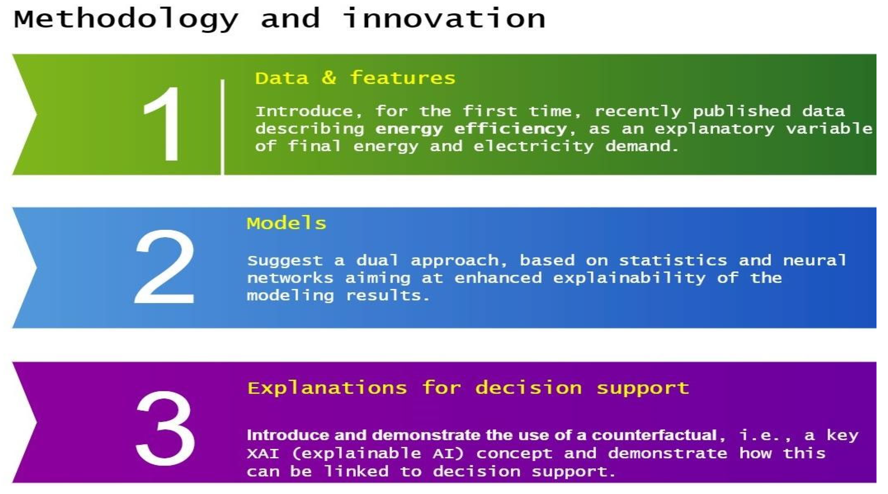
Figure 1 below illustrates the key points of the investigation and the innovation we introduce in dealing with the final energy and electricity forecasting.
2.1. Selecting Features for Total Energy and Electricity Demand Prediction with Interpretability in Mind
Burkart N. and Huber F.M. [
14] stress the importance of data quality and domain knowledge to create better explanations and improve the classification performance of the AI models. They state that ‘Explainability in the form of attribute importance conveys a sense of causality to the system’s target group. The concept of causality can only be grasped when the system points out the underlying input-output relationship’.
What would this mean in our case? How can we best address the feature selection so that we land as closely as possible to interpretable ANN models, to which counterfactual logic may then be applied? Our feature selection process will abide by the following criteria.
We will seek to include all major ‘causes’ of consumption; we will also try to include only one feature for every ‘cause’, avoiding double counting. Similarly, we will consider ‘causes’ as independently as possible, avoiding semantic overlapping as much as possible.
We will try to restrict the investigation to those features that are particularly relevant to our use and mid-term timeframe. For example, we will not include any dematerialisation feature, such as that attempted by Sun J.W. [
5], on the grounds that this will not significantly manifest over the mid-term, which is our key concern here.
We need to place a special interest in actionable features, i.e., features we can tweak and act upon. This is important in the case of decision support. For example, weather parameters are not actionable. They may significantly affect consumption, and may therefore fulfil above criterion 1 and deserve inclusion in our models; however, from the decision support perspective they cannot be acted upon.
Finally, data availability is also important and poses some important constraints. In a short-term investigation, we always have the option to generate the data we consider essential; in our mid-term timeframe, there is little chance to do so. One has to rely on data that can already be registered and trusted.
Following the above guidelines, we will discuss below the possible candidates for the cases of total final energy and electricity consumption.
2.1.1. Weather
The weather has an important causal impact on consumption (criterion 1 fulfiled), especially as regards space heating and cooling, which is a major final use of energy. It is also highly relevant to our mid-term timeframe (criterion 2 fulfiled). Indeed, weather cannot be acted upon (criterion 3 is not fulfiled), but due to its importance and also the easy availability of such data (criterion 4 fulfiled), weather will be included in the models by means of the heating and cooling degree days. Cloud coverage may also have an impact on final consumption as it affects lighting energy. However, this causal relationship is not as pronounced as the case of space heating; also, cloud coverage data are not available aggregated at a country level (criterion 4 not fulfiled).
Therefore, we will restrict the weather impact to the HDD/CDDs. In addition, we have opted to compact the data for HDDs and CDDs in just one indicator, called HCDD. It is well known that, owing to the more efficient thermodynamics (COP up to 4), cooling by one degree is less energy demanding than a respective heating of one degree. Researchers [
15] carried out an analysis of how exactly this difference develops not only in terms of the efficiencies of the end devices but also throughout the full heating/cooling energy generation process. They have proposed a value of two to express the life-cycle energy requirements of one degree of heating/one degree of cooling. Although this figure will certainly depend on the efficiencies of heat and electricity generation schemes in place, for the purposes of the current analysis, it is of adequate accuracy. Therefore, the weather will enter our models via the HCDD feature (1) calculated as follows:
where,
HDD: heating degree days,
CDD: cooling degree days,
HCDD: heating/cooling degree days, a compact indicator for modelling weather as a feature of demand prediction
2.1.2. Socioeconomics
We propose to cluster the socioeconomic features pertinent to our forecasting task in four feature categories: size, price, use intensity, and use efficiency. The first three are well highlighted in the literature discussed above; income is often mostly used for the intensity category, although as we will see below, different options are possible in residential sector investigations. In addition, data on use efficiency have started showing up in the literature and deserve some investigation. Below is a concise presentation of our approach as regards socioeconomic parameters.
Size
The size of the group of consumers/citizens is clearly relevant to consumption. In the ‘Size’ segment, we would use the population. Population is important (criterion 1), pertinent to our use case (criterion 2), and easily available (criterion 4). It is not an actionable feature; therefore, it cannot serve as the basis for counterfactual analysis (criterion 3 not fulfiled).
Price
It is fundamental that price affects demand. Although this is an unquestionable principle, the price elasticity of energy demand is an investigation for which results published and evidence accumulated remain, as we have seen in the Introduction, quite conflicting. Overall price is an important aspect of our investigation here (criterion 1), it is pertinent to our use case (criterion 2), and its historical data are relatively easily available (criterion 4). In addition, it is also an actionable feature (criterion 3 fulfiled), in the sense that a policy maker may act upon it: for example, via environmental taxes.
In addition, Eurostat household energy price data are split up so they show the basic energy price and the various taxes added to it. This allows us to possibly consider these components separately, isolating the impact of the ‘taxes’ applied. This applies both to the gas price as well as the electricity price.
Use Intensity
The intensity in using energy will be principally affected by a measure of development such as GDP per capita (PPP adjusted). This indicator would fulfil criteria 1, 2 and 4. It would bear a clear causal relationship with consumption, would be pertinent to our mid-term investigation, and would be relatively easily tracked as data. It would, however, not be an actionable variable and thus would not be able to support counterfactual analysis.
Intensity is also affected by major trends such as dematerialisation of the economy. Dematerialisation in energy is used to describe that ‘more is being achieved with less consumption of energy’ [
16]. However, as we have hinted in the introduction, this causal path is not likely to manifest in the mid-term and we will therefore not include it in our investigation, restricting solely to GDP per capita (PPP adjusted) figures as far as intensity is concerned.
Use Efficiency
Efficiency is a complex aspect to which citizen awareness, technology, and policies contribute. Odyssee Mure [
17] has developed an elaborate energy efficiency indicator [
18], called ODEX. It has been designed to measure the energy efficiency progress in industry, transport, households, and services as well as for the whole economy (final consumption). For each sector, the index is calculated as a weighted average of sub-sectoral indices of energy efficiency progress; sub-sectors being industrial branches, service sector branches, end-uses for households, or transport modes.
In short, ODEX calculation is based on two requirements. First, by expressing trends in specific energy consumption by end-use or sub-sector, as an index of change. Second, by calculating a weighted average index for the sector on the basis of the share of each end-use/sub-sector in the sector’s energy consumption. Interestingly, the indicator has not remained a theoretical construct but has been calculated and validated in all EU states using 1990 as a baseline. To this extent it is an indicator that fulfils our criterion 4 (data availability).
Though use efficiency may be important (fulfilment of criterion 1) and data of it have started being collected and reported upon (fulfilment of criterion 4), it remains rather unlikely that this impact may manifest at a mid-term timeframe such as the one considered here (unlikely fulfilment of criterion 2). Even more, it is well known that rebound effects may simultaneously occur as an improvement of energy efficiency [
19]. Such rebound effects may also be related to energy prices [
20].
Taoyuan W. and Yang L. [
21] have studied the rebound effects that accompany efficiency improvements. They investigate various types of efficiency and how they affect the flow of energy between production sectors and households, and impact upon the supply of labour and capital. They reached the conclusion that a 10% efficiency improvement will be typically absorbed by rebounding effects up to 68 to 76%. Seen from the emissions point of view, things are even worse. In the case of Japan and China, they estimate an almost similar increase in emissions as those reduced by the efficiency improvement, offsetting any impact of the improvement. In Russia, this emission rebound is lower, amounting to 75%. According to the authors, a well-organised economy would increase effective inputs of other resources in the economy to fully utilize the increasing energy services associated with energy efficiency improvement. In the long term, energy efficiency improvements are significantly reduced, although they may still promote considerable economic growth and social welfare through inducing an additional supply of labour and capital.
Still, the above results are not unanimously accepted. Nadel S. and Lowell U. [
22] also model rebounding in their approach, which they now estimate at a much lower level of 8% (the weighted average of 10% for the residential sector and 5% for commercial and industrial). In this way, they reach a vastly different result when stating ‘energy efficiency can reduce energy-related carbon emissions in the U.S. in 2050 by as much as 57% relative to current projections.’ Somewhere in between lies the approach of Gillingham et al. [
23]. These researchers estimate that the so-called microeconomic rebound is, in most cases, in the order of 20 to 40% when including all substitution and income effects, and perhaps even including the embodied energy in the energy efficiency improvement. They also acknowledge that macroeconomic rebounding is far less understood. They also conclude that while the energy savings from energy efficiency policies will be reduced by the presence of a rebound effect, efficiency-oriented policies are likely to conserve energy, besides of course increasing welfare.
Efficiency is a cognitively different and highly important dimension of energy demand. One should not understate the apparent complexity of the issue, especially as regards the associated rebound effects, and the lack of data to model them. Additional difficulties are introduced by the link of efficiency with pricing and the rather lengthy time horizon over which policy decisions targeting efficiency may turn into tangible results.
The ODEX indicator provides a data-backed approach to efficiency. Indeed, we used the ODEX data in the modelling but, as we will discuss below, failed to track any statistically significant impact.
2.2. Possible Adaptations for the Residential Sector
The approach of the above paragraph can be used in the case of household sector consumption patterns. In the case of ‘weather’, ‘price’, and ‘efficiency’ no changes would be required. In the case of ‘size’ and ‘intensity’ one can also look into alternative feature selections, as discussed below.
In the case of ‘size’, it seems that there are alternative ways to model size, for example in terms of the ‘total floor area of dwellings’. Likewise, in the case of intensity, besides GDP/capita, we would argue that ‘average private household consumption’ could provide an alternative for the energy use intensity. ‘Dwellings’ area per capita’ could also be a valid formulation of the intensity indicator. Data are available for both these alternative features, through the same source referenced above [
11,
17].
2.3. Summary of the Feature Discussion
The following table summarises the data that will be used in the mid-term forecasting of final consumption and electricity in the residential sector. Data sourcing is also illustrated in the table.
The analysis that follows below aims at isolating the most promising features. Arguably no matter how much we have tried to define independent features, there will still be many interdependencies among them, something that will manifest in terms of high collinearity indices. Thus, a number of trials were necessary to end up with the minimal set of features, providing a satisfactory model while suppressing collinearity. The data approach will be discussed below.
3. Evaluating the Features in Terms of Statistical Significance
Data for the candidate features were sourced from EuroStat (energy database) and Odyssee Mure, a project that hosts energy related data and monitors energy efficiency trends and policy measures in Europe. The statistical analysis was based on linear regression and was carried out in JASP. Below we will present the detailed data and analysis in the case of the Netherlands and the compact results for all other countries. However, all data of all countries have been shared on OSF (Open Science Foundation,
www.osf.io, last access 4 July 2021) and are fully accessible under the public project ‘JASP analysis of national energy forecasting’. The results can be directly seen on JASP. Access to the raw data will require first downloading the file and then opening it in JASP.
As far as the statistical treatment is concerned, various feature combinations were tested and a minimal set was retained. No counter-intuitive coefficients showed up in the regression equation; no special action or elaboration was therefore necessary as regards this important aspect of the forecasting.
Additionally, a further important consideration was to retain only features that entered the equations with a low p-value, signalling a good statistical significance of it. Furthermore, features that, upon inclusion, displayed a high collinearity as reported by the SVI indicator were excluded. Collinearity means that the introduction of a new feature does not introduce independent information; it is somehow already correlated with one of the other predictors.
4. The Case of the Netherlands: The Data
Guided by
Table 1, the following table illustrates all the pertinent data collected for the case of the Netherlands from the Odyssee [
17] and Eurostat [
24] databases.
5. The Case of the Netherlands: The Results
Based on the methodology presented in and the data collected and shown in
Table 2, we present below the results for the Netherlands, in the case of residential final consumption as well as electricity consumption.
5.1. The Case of Final Consumption
Table 3 illustrates the results of the analysis for final energy consumption, in the case of the Netherlands.
HCDD, taxes on gas, and the consumption per capita have been found to yield the best results, based on the low p-values, the acceptable collinearity statistic (VIF), and the adjusted R2. Additionally, the predictors enter the regression with the correct sign: negative for the taxes, as their increase will lower consumption; positive for HCDD and the consumption per capita, as a harsh winter and an increase in purchasing power, respectively, are expected to increase final consumption.
5.2. The Case of Electricity
Table 4 illustrates the results of the analysis for electricity consumption, in the case of the Netherlands.
The best fit was achieved via GDP/capita alone. In the case of electricity, taxes, and weather, as well as all other candidates of
Table 1, they did not add to the model quality as
p-values or the VIF statistic rose significantly with no accuracy benefit.
6. The Results for All Countries: Final Consumption and Electricity
Below, the compact results for all investigated countries are presented. Please note that in the case of Greece and Portugal gas-related data were not available so only electricity forecasting was attempted. Below, in
Table 5, the compact results for all investigated countries are presented, for the case of final energy consumption. Please note that in the case of Greece and Portugal gas-related data were not available so only electricity forecasting was attempted, (
Table 6).
Below, in
Table 6, the compact results for all investigated countries are presented, for the case of electricity consumption.
Table 6.
Summary results for the residential electricity consumption forecasting in all six countries investigated (NL, SE, ES, DE, PT, EL).
Table 6.
Summary results for the residential electricity consumption forecasting in all six countries investigated (NL, SE, ES, DE, PT, EL).
| Country | Best Predictors | Standardised Coefficients | Adjusted R2 | p-Value | VIF |
|---|
| NL | | | 0.936 | | |
| 1 | GDP/capita | 0.968 | | <0.001 | 1 |
| SE | | | 0.639 | | |
| 1 | HCDD | 0.730 | | <0.001 | 1.079 |
| 2 | Population | 0.620 | | <0.001 | 1.079 |
| ES | | | 0.981 | | |
| 1 | Taxes Electricity | −0.180 | | 0.001 | 3.489 |
| 2 | Dwellings’ Area | 1.138 | | <0.001 | 3.489 |
| DE | | | 0.422 | | |
| 1 | Taxes Electricity | −1.065 | | <0.001 | 2.935 |
| 2 | Dwellings’ Area/capita | 1.141 | | <0.001 | 2.935 |
| PT | | | 0.935 | | |
| 1 | Dwellings’ Area | 0.749 | | <0.001 | 4.495 |
| 2 | Taxes Electricity | −0.423 | | <0.001 | 2.606 |
| 3 | Consumption/Capita | 0.557 | | <0.001 | 2.483 |
| EL | | | 0.884 | | |
| 1 | HCDD | 0.208 | | 0.027 | 1.526 |
| 2 | Dwellings’ Area/capita | 0.809 | | <0.001 | 1.526 |
7. The Neural Network (NN) Based Prediction Model
Following the above analysis, we constructed neural network models based on what the statistical analysis revealed as the best predictors. In this way, statistical analysis served as a first level of result interpretability, allowing us to highlight and gain insight into the inferences in place. After this, the prediction power of NNs was called upon to calculate prediction accuracies.
The Tensorflow machine learning library [
25] was used to assist this investigation. Neural networks were created with the above-discussed input and output layers, with two hidden layers in-between. The data were split in two parts; 70% were used as training data to develop the model and 30% as testing data to calculate its accuracy. The results are presented in the following table.
In the above table, MAPE is the mean average percentage error and RMSE is the root mean square error. They are calculated with the following formulae
where
At is the actual test value,
Ft the related forecast value of the model, and
n the size of the test data.
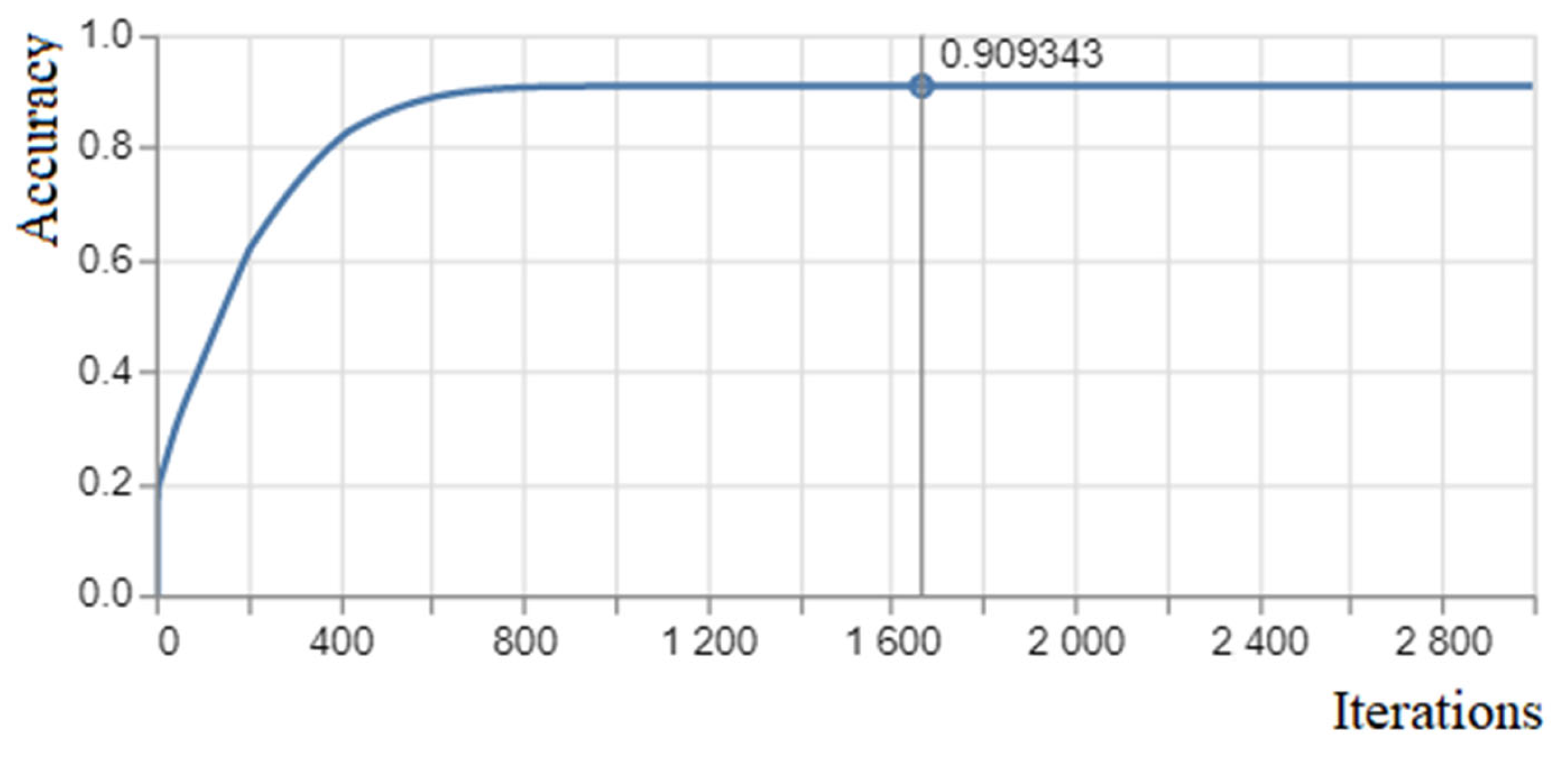
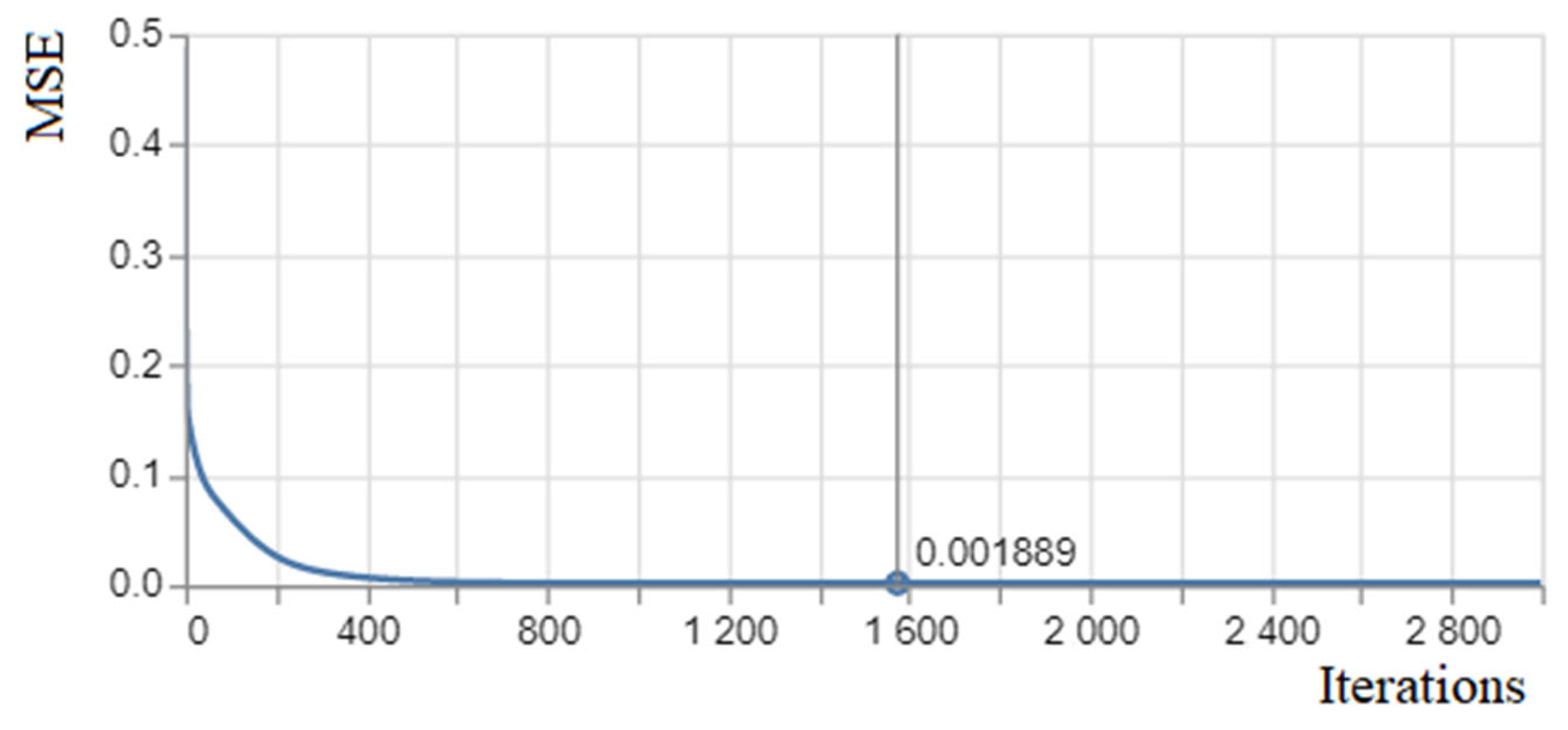
Convergence typically required between 500 and 1000 iterations following which the model error metrics ceased to change. The figure below illustrates this in the first of the cases reported above (final consumption/NL). Similar results apply across all models developed.
The software produced diagrams of the MSE, which when square rooted yielded the RMSE figures reported in
Table 7.
8. Results and Discussion
As expected, the ODEX energy efficiency indicator did not introduce quality or accuracy to the modelling. For example, in the case of Germany, when introduced as an additional parameter in the case of final consumption, the
p-values and the VIF statistic deteriorated, as shown in the table below. Additionally, the sign on the taxes reversed to a positive number, which is counter intuitive and therefore unacceptable.
Table 8 illustrates the results when the energy efficiency indicator was used as an exploratory variable.
As regards the other four broad candidate predictors of
Table 1, in no case did all four of them result in the best possible performance. In most cases, collinearity rose significantly, indicating that no true independent information was introduced to the model. Thus, the best number of predictors varied between two and three, and in one case was as low as one. In most cases, the intensity of use and the size-related features were found to be strongly correlated, and one of them had to be removed. Only in the case of electricity in Portugal did a size-related feature (dwellings’ area) appear in the best model along with an intensity feature (consumption/capita).
The accuracy of the ten linear regression models (four for final consumption and six for electricity) was generally high, with the notable exception of Germany. A possible reason for this is that in the 1990s and during the integration of the Eastern regions of the country, Germany experienced a rare transition period whose socioeconomic characteristics were fluid and very particular to the moment. Another case of relatively low accuracy (adjusted R2 = 0.639) was that of electricity in Sweden. Indeed, a good understanding of the local socioeconomics and markets is required in order to have more insight in the results, not only with regard to the accuracy but also to the features that prevailed as key drivers of consumption, final and electricity alike.
Weather appears to be an important predictor of final consumption in all four countries. In particular, in two countries (Germany and the Netherlands), it appears to be the most important predictor, when considering the values of the standardised coefficients of the regression. In the case of electricity, this correlation is pronounced only in the case of Sweden and in Greece; in the other four countries, the weather was not found to add true explanatory value to the models. This is quite predictable, as weather affects heating and cooling, which typically runs on gas and not on electricity.
An important result is related to the impact of energy taxes. As we have argued above and illustrated in
Table 1, this feature is the only actionable one. In this work, we have found that taxes burdening the energy price appear to be an important predictor. They demonstrated a strong correlation with final consumption in all four countries. In no case was the base price of energy found to be a better predictor than that of the taxes burdening the energy. However, in the case of electricity, the tax impact is not as clear. Only in three of the six countries did taxes introduce accuracy without undermining the model quality via high
p-values or VIF statistics.
The neural network-based regression produced results in line with the statistical regression. With the exception of Germany again, the accuracy achieved in all the other cases, nine in total, was good.
As expected, in this case of the NN regression, accuracy was improved. As JASP reported an RMSE based on all the data, without splitting the data into modelling and testing sets, we had to carry out this exercise manually. For example, in the case of electricity consumption in Sweden, JASP reported an RMSE value of 0.078. Then we split the dataset in the years 1996 to 2010 for the model development and used the model to predict the remaining data (2011 to 2018). The RMSE naturally increased to 0.118. The respective ‘true’ RMSE for the NN model was found to be 0.095, which is about 25% lower than this figure.
This confirms that the NN approaches are superior in terms of accuracy. However, by using first a statistical approach to better understand the underlying inferences, we combined the advantages of both worlds: insight and accuracy.
8.1. Linking to Decision Support
A possible important decision that could be supported by means of the above investigations would be:
‘What is the best action that I should take in order to achieve an x% reduction of greenhouse emissions in the mid-term horizon?’
Such questions are typically addressed using counterfactual analysis. A counterfactual explanation of a prediction describes the smallest change to the feature values, which changes the prediction to a predefined output. Counterfactual analysis is also referred to as local interpretability in the sense that it does not aim to propose some general surrogate and more transparent model in the place of the typical black box of the neural network. Instead, it aims at addressing ‘what if’ type questions and finding the minimal tweak of the model features that could secure this new goal.
A first step towards interpretability is the selection of features via a statistical analysis, as shown above. This process allows us to gain insight into what really matters. An NN model would not provide any such service. A next step for local interpretability would be to lay out a counterfactual analysis allowing us to address questions such as the one above.
If we are to realistically tweak model features to perform ‘what if’ analyses, it is critical to identify the actionable features. One cannot possibly change the weather by reducing the GDP/capita. In our case, the only possible actionable feature pertinent to our decisions here is that of energy taxes. Indeed, taxes in our analysis appeared in most cases as a key driver of consumption.
At this point, we should recall that there is an ongoing debate in the literature as to if and how much taxes can affect consumption. First, we have to acknowledge that not all societies respond in a similar way to taxes. Then there is always the possibility that there is a confounder to taxes; some other parameter that is truly causing the change, but as it moves in line with prices, one may end up with the wrong impression that it is prices that are driving consumption.
Along this line of thought, a good example is provided by Borestein Severin (2019) [
26], who is in favour of using the energy pricing mechanism. He argues: ‘accounting for externalities requires introducing the 50 usd/ton CO2. The trend that taxes have shown convinces this will have an impact. Perhaps not direct—by immediate behavioural change—but by long-term driving for more innovation.’
Indeed, prices bundle together three types of impact: the immediate behavioural response, a gradual behavioural change, and an impact on innovation. Perhaps the immediate response is not as strong, and perhaps this is why in the literature, there is often a claim for an essentially inelastic demand. However, how inelastic can demand be to price if it can trigger innovation or more mid-term behavioural shifts? Can we really claim that consumption is inelastic to prices if prices are driving innovation?
Below, we perform some counterfactual analysis on the results achieved via tweaking energy price/taxation. The table below illustrates the taxation change that would result in a 5% reduction of consumption in the seven cases overall, where taxation was found to be a driver of consumption. Both linear regression and NN models are reported.
The counterfactual analysis has been performed using the DiCE (Diverse Counterfactual Explanations) framework [
27]. The framework generates counterfactual explanations for any machine learning model, including the neural networks.
8.2. What-If Scenario for a 5% Decrease in Final Consumption via Taxation
Table 9 presents the results of the taxation counterfactual analysis for both modelling approaches (linear regression, NN). Taxation appeared to be an important predictor in all four cases investigated for residential final consumption.
8.3. What-If Scenario for a 5% Decrease in Electricity Consumption via Taxation
Table 10 presents the results of the taxation counterfactual analysis for both modelling approaches (linear regression, NN). Taxation appeared to be an important predictor in three out of six cases investigated for residential electricity consumption.
Counterfactual analysis showed that the hardest change to decrease final consumption is for Sweden, which requires a 72.3% tax increase. The electricity consumption case showed that Germany requires the biggest tax increase of 69.2% to obtain a lower electricity consumption estimate, whereas Portugal needs only a 3.2% increase.
The NN counterfactual analysis for Germany failed to converge, something related to the poor models for this country, especially in the case of electricity.
Last, counterfactuals on the linear regression and the NN models yielded quite similar results, although it is notable that the NN models required higher levels of tax increase in all but one case, where the results were exactly the same (electricity consumption in Spain).
Above, we have restricted the analysis to households. However, imagine we could have similarly constructed models for the other two broad categories of energy consumption: transport and business/industry. In this case, our decision would also be informed by the other two models and would require cross model counterfactuals, able to tweak all actionable features they may include, to find the least change and action required in order to achieve our end goal, as articulated at the beginning of this section. It would be able to support energy policy decisions in a much more comprehensive way.
One should also note that while the residential counterfactual presented above is, from a technical point of view, easy to elaborate and implement, this multi-model counterfactual would represent an AI challenge.
9. Conclusions and Policy Implications
This paper provides data and modelling insights into final energy and electricity consumption in the residential sector, with the main and practical end purpose to support mid-term energy planning. All pertinent and available data from six countries from various parts of the EU have been collected and put together to develop the models.
In the analysis, we have tried to introduce and highlight the emerging concept of model interpretability: the idea that now we must not blindly rely on black box approaches typical of machine learning and especially pronounced in the case of neural networks but strive to gain insight into the model workings. This underpins the model construction where we have carried out a preliminary statistical analysis to understand the underlying inferences, before engaging in neural network-based predictions. The latter have indeed resulted in satisfactorily high prediction accuracies. Interpretability also includes the so-called counterfactual analysis, whereby one seeks to define the least tweaking of actionable features required to produce a given output (consumption reduction in our case).
We have attempted to introduce energy efficiency into the models, as encapsulated in the recently defined ODEX indicators. However, this did not add to the quality and accuracy of the models. Apparently, rebound and dematerialisation effects are in action and counteract the efficiency gains. This is particularly the case in the current residential context. We suspect that this might not be the case in transport or industry consumption, where the high residential rebound effects might be less pronounced, and we look forward to soon carrying out this investigation.
Price and its elasticity is a much-debated issue; in the six countries studied, we have found in most cases quite a significant impact, in terms of the respective, standardised regression coefficient, of energy taxes on consumption. However, it is hard to say to what extent this is owing to immediate consumer response, more mid-term behaviour change, or the triggering of innovation, all of which receive some credit in the literature.
In view of the energy transition and the growing pressure to curb carbon emissions, a fully-fledged energy policy support scheme in this direction would require similar investigations and developments also in the direction of transport and industry. Putting in place forecasting models in all three energy categories (households, transport, and business/industry) is the first requirement to run so-called ensemble model counterfactuals, ending up with suggestions as to the most promising actions (see
Figure 4). As the word implies, action will require actionable features, and taxes is an especially prominent one. In the case of households, in fact, it is the only one; the other two cases are still under investigation.
Of course, to expand decision support beyond sheer energy demand forecasting to also encompass greenhouse reduction considerations would also require the local energy system layout. Indeed, greenhouse gas emissions are not related only to energy consumption; more precisely, they are related to fossil-fuel-driven energy consumption. Thus, possible environmental taxes should take account of this layout and burden consumers according to the life-cycle emissions per consumed kWh.


