1. Introduction
Appropriate water management is essential for implementing Sustainable Development Goals (SDGs). Management of surface water includes maintaining its desired quality. Often, surface water is the only source of water supply for cities and villages [
1], where low water pH value may lead to serious problems in the water treatment system. Such water contains increased concentrations of pollutants due to sediment dissolution in the lake bottom, frequently needing additional resources (chemical reagents, additional purification equipment) for the water treatment stations [
2] required to purify surface waters following the existing standards. The issue can be solved using natural limestone, a secondary product of limestone quarries [
3]. The use of limestone to maintain water pH within the neutral values will allow the water treatment plant to operate without the use of additional resources [
4,
5]. In addition, the application of dispersed, thermally active limestone may help reduce the accumulation of secondary products of limestone quarries. Thus, land use (use of secondary products of limestone quarries) has an impact on water use, with a cascading effect on reducing the use of additional resources for water purification.
Low pH of surface water can be a consequence of anthropogenic influence (eutrophication) and is one of the most common causes of water quality deterioration [
6]. The problem of low pH value can be solved using CaO, Ca(OH)
2, Na
2CO
3, and limestone CaCO
3 additives [
7,
8]. The use of limestone CaCO
3 has several advantages over CaO due to the fact that the addition of CaO increases water temperature since its interaction with water is an exothermic reaction. The use of Ca(OH)
2 also has a number of limitations associated with the preparation of its solution and the use of dispensers. Moreover, when added to water, its pH value can increase sharply and lead to chemical burns of flora and fauna. Na
2CO
3 is also applied for the neutralization of natural waters [
9]. The disadvantage of using this material is its high price compared to natural limestone. The use of CaCO
3 provides longer-lasting changes in water pH value compared with other neutralizing materials such as CaO, Ca(OH)
2, Na
2CO
3.
When in water, limestone dissolves slowly and therefore, the increase in water pH does not cause chemical burns of flora and fauna [
10]. In addition, carbonate can be an important source of CO
2 for photosynthesis in water, and thus crucial for the bioavailability decrease in toxic divalent cations of heavy metals (e.g., Ni, Cd, Cu, Pb, Zn) due to the formation of insoluble complexes with metals [
11,
12,
13,
14]. Furthermore, accurate liming practices often result in decreased mercury contents in fish [
15].
Limestone is the best and most frequently used neutralizing agent for treating acidified surface waters worldwide, and the recommended limiting doses are indicative. The most commonly used doses of fine-grained limestone are in the range of 750–1000 kg/ha (for the typical depth of natural lakes at 1.0–1.2 m). The dose of limestone from the proposed range depends on water pH level and sediment type in the reservoir bottom. A smaller dose is applied when the bottom is sandy and a higher dose when the bottom is muddy [
16].
The Swedish Liming Programme recommended another approach to determine the dose of limestone [
17]. The dose depends on water pH and retention time; for lake water, the dose is 10–75 g/m
3, and for watercourses—10–30 g/m
3. Liming of lakes by adding doses of 10–30 g/m
3 should be repeated before the pH level exceeds 6. Mathematical models can be applied to calculate limestone dosages [
18].
Liming of surface water is not always mandatory, but EPA recommendations should be followed if necessary. According to these recommendations, with a single application of limestone, the pH increase should not exceed 1.5 [
19]. It is very important to consider that when limestone is added to water, the pH increase can also be high. Therefore, before adding limestone to surface water, all factors that increase the pH value [
20] must be considered. These factors include initial pH values, total mineralization, redox potential, and limestone dose [
21,
22]. The pH value and total water salinity affect the solubility of minerals. When the initial pH value is lower, more minerals are dissolved, resulting in a pH increase. The same pattern is observed when the mineral is dissolved in water characterized by different mineralization. Analysis of these factors coupled with experimental studies helps determine the optimal dose of limestone needed to reduce water pH following EPA recommendations.
Trach et al. [
23] studied the change in water pH in relation to the dose of natural limestone. With the increase in the initial water pH values (from 3 to 7) and mineralization (from 0.01 to 0.53 g/dm
3), the required dose of limestone decreased. The results of experimental studies have shown that with lower initial water values (pH and mineralization), the required dose of limestone is also lower. To increase water pH to a neutral value (pH ≈ 7) and ensure the safety of this process, the limestone must be added to water several times at specific intervals. Such interval is necessary for adapting flora and fauna after the increase in pH and water salinity. In addition to water pH and salinity, the pH change with limestone also depends on water Eh [
18]. The value of this water parameter depends mainly on the amount of organic matter.
Next, the existing experience of using ANN in ecological engineering was analyzed. The application of ANN for modelling time series of total phosphorus concentration was described for the Odra River conditions [
24]. Using sensitivity analysis, a relationship was established between phosphorus concentrations and other water quality variables. Two models were created to predict phosphorus concentrations, with one input variable and fourteen input variables. Both ANN models showed good predictive ability with new datasets.
Furthermore, the ANN model was applied to forecast the concentration of total nitrogen and total phosphorus in the lakes from the United States [
25]. ANN models were trained, tested, and validated using three inputs (pH, conductivity and turbidity) that were statistically correlated with the output data. The study results showed that ANN modelling is a good tool for assessing nutrient concentrations in lakes.
Van et al. [
26] predicted the concentration of dissolved oxygen in a river setting based on hydrological parameters (temperature, pH, turbidity, conductivity, chemical oxygen demand, biological oxygen demand, nitrate and phosphate). Multivariate regression (MLR) and backpropagation neural network (BPNN) methods were used to establish these relationships. The results of their study showed that the BPNN might accurately predict the concentration of dissolved oxygen in the water.
Stamenković et al. [
27] developed an ANN model to predict the concentration of nitrates in river water. Their model was trained and tested on 26 input water quality parameters. The results obtained showed the ability of ANN models to predict the concentration of nitrates with an average absolute error of 0.53 and 0.42 mg/dm
3 for the test data.
Krtolica et al. [
28] constructed a multilayer feed-forward ANN model using macrophytes as independent variables for each water quality variable (dissolved oxygen, nitrate-nitrogen, and orthophosphates). They selected 28 macrophytes as key water quality indicators by sensitivity analysis for one environmental variable. The developed ANN architecture presented a modelling approach that can be applied in different biological systems.
Gebler et al. [
29] performed ANN modelling of macrophyte indicators depending on the physicochemical water parameters. They analyzed several indices of macrophyte diversity (species richness-N, Shannon’s index-H, Simpson’s index-D and Pielou’s index-J), as well as the ecological status index (macrophyte index for rivers-MIR). Alkalinity, conductivity, pH, nitrate and ammonium nitrogen, reactive and total phosphorus, and biochemical oxygen demand were used as the input variables. The quality of the constructed models was assessed using the calculated errors and the Pearson correlation coefficient.
Chen et al. [
30] developed three models for estimating the concentration of dissolved oxygen: backpropagation neural network (BPNN), adaptive neural fuzzy inference system (ANFIS), and multilinear regression model (MLR). The input variables of the neural network were water temperature, pH, conductivity, turbidity, suspended solids, total hardness, total alkalinity, and ammonia nitrogen. The performance of the models was assessed using the mean absolute error, root-mean-square error, and correlation coefficient. Comparative analysis of the models showed that ANN had the best performance characteristics.
In the study performed by Wen et al. [
31], the authors used a three-level backpropagation ANN with a Bayesian regularization learning algorithm. The input variables of the neural network were pH, conductivity, chloride (Cl
−), calcium (Ca
2+), total alkalinity, total hardness, nitrate-nitrogen (NO
3−N), and ammonia nitrogen (NH
4−N). The values of obtained correlation coefficient and root-mean-square error showed the effectiveness of the ANN model.
Singh et al. [
32] described the training, validation, and application of ANN models to calculate dissolved oxygen levels and biochemical oxygen demand. Their models used eleven input water quality variables measured in river water. The efficiency of ANN models was assessed using the coefficient of determination (
R2) and root-mean-square error, calculated based on values of the output variables measured and calculated in the models. The authors summarized that ANN models could be used to calculate water quality parameters.
Csábrági et al. [
33] aimed at predicting the concentration of dissolved oxygen based on easily measurable parameters of water quality (pH, temperature, conductivity) and runoff. Four linear and nonlinear models were adapted, i.e., multivariate linear regression model, multilayer neural network (perceptron), radial base function neural network, and general regression neural network model. The performance of the models was evaluated using various statistical indicators. Nonlinear models gave better results than linear ones. To determine the parameter that had the most significant impact on the performance of the models, the authors conducted a sensitivity analysis, which showed that for all three neural network models, pH played the most important role in estimating the content of dissolved oxygen.
As indicated above, ANN has been successfully used for modelling various physicochemical processes in different site conditions. This is because most environmental processes are nonlinear due to their complex chemical and physical nature. Nevertheless, the task of assessing the permissible pH level when adding limestone to water has not been fully accomplished.
This article is an interdisciplinary research paper aiming at:
- (1)
Determination and comparison of the doses of new dispersed, thermally activated limestone and natural limestone,
- (2)
Finding the relation of dose value to initial water parameters (pH, Eh and total mineralization values).
- (3)
Creation of a model using artificial neural networks (ANN) to predict changes in water pH values in line with EPA recommendations.
The doses of dispersed, thermally activated limestone were determined, taking into account EPA recommendations, the use of which has an advantage over natural limestone. The limestone application helped to reduce the accumulation of secondary products of limestone quarries.
In addition, the systematization of various scientific directions in one study is the scientific novelty of this research.
2. Materials and Methods
2.1. Materials
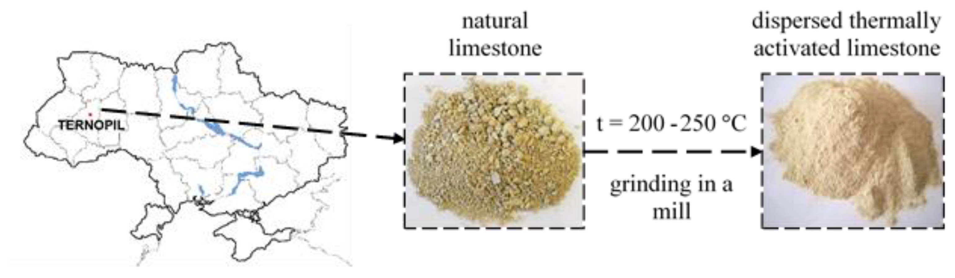
The material used in the study was dispersed, thermally activated limestone mined in a quarry in Ternopil, Ukraine (
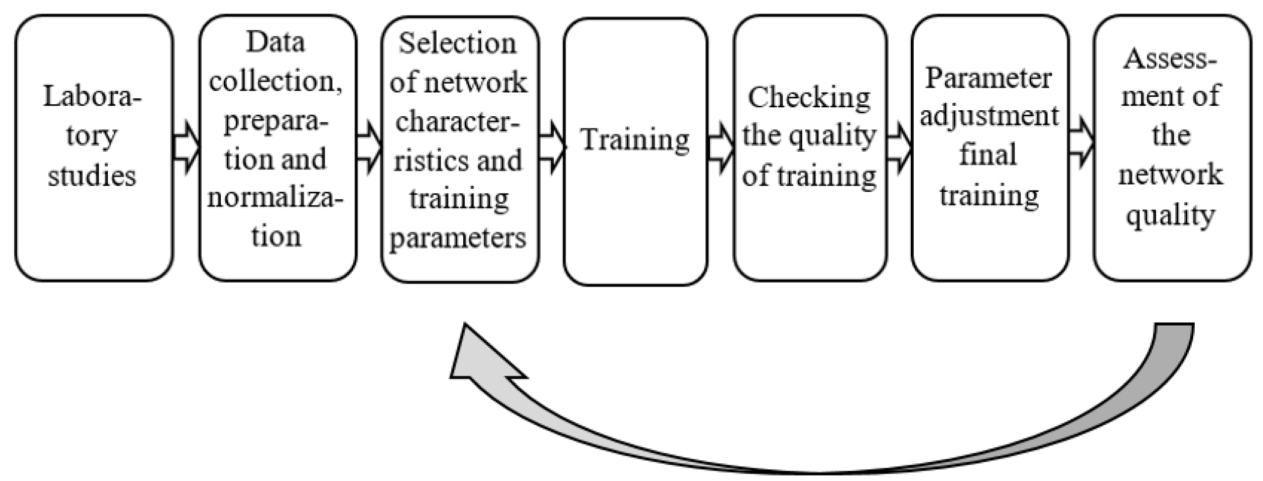
Figure 1). Preparation of such limestone in the Ternopil Quarry enterprise is carried out according to a specific algorithm (
Figure 2). Directly at Ternopil Quarry is an accumulation of fine fractions (0–40 mm) of carbonate rocks, which do not satisfy the requirements for building mortar fillers and are unsuitable as building stone. Therefore, the enterprise produces dispersed limestone from unused limestone screenings. Such limestone is used as a Ca-rich mineral fertilizer.
The raw materials for the production of dispersed limestone are primary and secondary crushing screenings with sizes up to 40 mm. Wet limestone is loaded into a shaft dryer. The gas temperature at the dryer entrance is 200–250 °C, and at the dryer exit-100–120 °C. A pipe is used for drying and separating the material that is 1 mm in size. Particles larger than 1 mm settle in the pipe and are sent for grinding in a hammer mill, after which they return to the drying pipe. This technological process produces dispersed, thermally activated limestone with a grain size below 0.001 mm.
2.2. Methods
As input values of the model, the following parameters were used: pH, redox potential (Eh), total dissolved solids (TDS), and various doses of dispersed, thermally activated limestone. For experimental studies, the applied doses of limestone were at 0.025, 0.05, and 0.1 g/dm3. Initial water pH values were 4.0, 5.0, and 6.0, Eh was 120, 280, and 420 mV, TDS was 0.02, 0.240, and 0.56 g/dm3. Experimental studies were performed at a temperature of 15 ± 0.5 °C.
Experimental studies were carried out under static conditions. A magnetic stirrer (model JNE FK-25W) was used to mix water and the analyzed limestone at a mixing speed of 0–2400 rpm and a maximum mixing volume of 3000 mL.
The changes in pH and TDS were determined using a multimeter (Milwaukee MW802, Rocky Mount, NC, USA). Eh was measured using an ORP meter (Milwaukee MW500 PRO, Rocky Mount, NC, USA). The MW802 has TDS measuring ranges up to 4000 ppm (4 g/dm3). The pH measuring ranged from 0.00 to14.00. Graduation was set as 0.10 pH, 10 ppm (0.01 g/dm3). Accuracy (25 °C): ±0.20 pH, TDS: ±0.02% of full scale. MW500 PRO measures Eh in a ±1000 mV range. The accuracy is at (25 °C): ±5 mV. Total dissolved solids (TDS) represent a measure of the dissolved combined content of all inorganic and organic substances present in a liquid in molecular, ionized, or microgranular (colloidal sol) suspended form (g/dm3). TDS concentrations are often reported in parts per million (ppm) or mg/L. Water TDS concentrations were determined using a digital meter. Before starting a series of measurements, the multimeter was calibrated using three buffer solutions (pH values at 4.00, 6.86 and 9.01), according to the recommendations for their use to ensure measurement accuracy. To adjust the required initial pH values, Eh and TDS, 0.1 M HCl, 0.1 M NaOH, and a potassium humate solution were applied. For experimental studies of the dependence of limestone dissolution on water Eh, a 10% solution of potassium humate was prepared. Chemical characteristics of potassium humate were as follows: water solubility (dry basis) —100%, humic acid (dry basis)—60%, fulvic acid (dry basis)—10.0–15.0 %, and potassium (K2O dry basis)—10.0%–12.0%, moisture—15.0%.
2.3. ANN Modelling
ANN can be thought of as a system of interacting artificial neurons. Connected in a large network with controlled interactions, neurons can solve fairly complex problems. The advantage of neural networks over mathematical methods is that they can look for patterns in fuzzy data, learn and systematize solutions. A neural network can generalize and highlight hidden dependencies between input and output data. Once trained, the network can predict future values based on previous values and various existing factors.
Within the framework of this study, data were collected, analyzed, and prepared, four ANN models were created, and a comparative analysis of their effectiveness was carried out. Normalization of input variables and ANN modelling, training, and testing were performed using the Keras library in the Python programming language. The results were visualized using the Matplotlib library in the Python programming language.
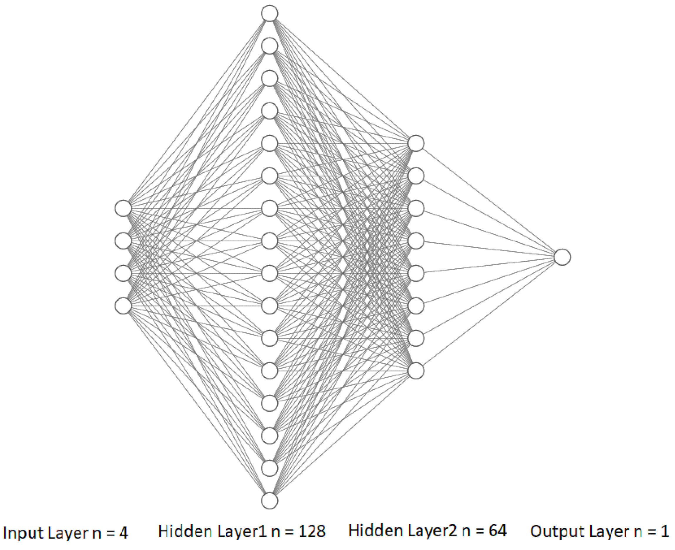
The ANN architecture proposed in this study has one input layer, two hidden layers and one output layer of neurons. The neural network architecture is a specific neuron arrangement and connection. The scheme of ANN architecture used in this study is shown in
Figure 3. The input layer consists of four variables, the first hidden layer has 128 neurons, the second hidden layer has 64 neurons, and the output layer consists of one neuron.
The number of hidden layers and neurons was determined empirically. Initially, one hidden layer of neurons was used (n1 = 128); in this case, the model showed a large error (MAPE = 48.3%). It was decided to increase the number of hidden layers and neurons (n1 = 128, n2 = 64). This led to an improvement in the ANN model performance with a slight increase in the calculation time.
In the first stage of ANN use, input layer neurons get an input signal and send an output signal to the hidden layer neurons. The neurons in the hidden layer calculate activation and send a signal to the neurons in the output layer. For an ANN, the total input signal is calculated by the formula [
34]:
where:
are input variables,
are weights.
The neurons of the output layer calculate activation and send the input signal. The activation function is used to calculate the neuron activation. In this study, ANN models were tested using two activation functions: the sigmoid (logistic) function and the ReLU (Rectified Linear Unit).
The sigmoid function is a smooth, monotonically increasing nonlinear function, which is defined as [
34]:
This function can be used in neural networks with many layers, as well as train these networks using the backpropagation method. The sigmoid function has the advantage of normalizing the output to the range (0, 1). This is useful when the resulting layer value must represent the probability of a random variable.
Recently, the ReLU activation function has gained wide popularity. If the argument takes a negative value when calculating this function, then the function is equal to 0; in the case of a positive value of the argument, the function returns the number itself:
The advantage of ReLU is activation sparsity. In networks with a large number of neurons, the use of the sigmoid function entails the activation of almost all neurons, which can affect the model performance. When using ReLU, the number of included neurons becomes smaller due to the function characteristics, and the network itself becomes more productive.
The next stage of ANN operation is the calculation of the loss (error) function. The loss function measures “how good” the neural network is for a given training set and expected responses. The loss function is responsible for assessing how well the model predicts the real value, and building the model comes down to solving the problem of minimizing the value of this function at each stage. The calculation of the loss (error) includes comparing the actual and target values for each neuron. The ANN learns until it achieves the global minimum error between the actual and target data.
In this study, the Mean Square Error (
MSE) was used to calculate the loss function:
where:
is the output calculated by the model, is the target output.
The squared deviation is calculated for each dataset, after which the resulting values are summed up and divided by the total number of datasets. The closer the obtained value is to zero, the more accurate the model is. This calculation method is highly sensitive to outliers in the sample or samples where the range of values is large.
For the appearance of overfitting, the early stop method was used [
35]. Training the network stops when the monitored metric no longer shows improvement. The monitored metric was validation loss. A training loop checks whether the loss no longer decreases at the end of every epoch. In such a case, the training stops.
Various methods can be used to minimize the loss function. In this study, two gradient descent methods were tested to optimize ANN training: Stochastic Gradient Descent (SGD) and Adaptive Moment Estimation (Adam).
The SGD algorithm updates the neural network weights using a single training sample at each step [
36]. SGD does not perform unnecessary calculations since the loss function is calculated not for the entire training set but only for one example. This contributes to the algorithm learning much faster. However, because at each step of the algorithm, the gradient is calculated based on different sets of initial data, updates of the weight coefficients are accompanied by frequent fluctuations of the objective function. Thus, on the one hand, SGD allows to move to potentially better local minima quickly, but on the other hand, large fluctuations significantly slow down the convergence.
According to Kingma and Ba [
37], Adam’s method is computationally efficient, requires little memory, is invariant to diagonal scaling of gradients, and is well suited for large data and parameter problems. The rule for updating the weights in Adam’s method is determined by using estimates of two different moments; the first uses the previously calculated values of partial derivatives, and the second uses their squares.
In this study, to assess the performance of the ANN models presented, the quality metric Mean Absolute Error (
MAE) was used.
MAE is the average sum of the absolute values of the difference between the real and predicted values [
38]:
The metric functions are similar to loss functions, except that the results of the use of the metric function are not applied in the model training.
MAE is similar to MSE in many ways but is less sensitive to outliers. The main reason is that in MSE when squaring errors, the outliers (which usually have higher errors than other samples) dominate the final error and affect model parameters.
One of the primary tasks of this study was the choice of the optimal ANN model. For comparative analysis of the accuracy of four neural networks, the Mean Absolute Percentage Error (MAPE) and the Coefficient of determination (R2) were used.
MAPE is a ratio defined by Formula (6) [
39]:
R2 is a statistical measure used in various models, for example, for predicting future outcomes or testing hypotheses based on other related information.
R2 provides a measure of how well the observed results are reproduced by the model, based on the proportion of the total variation in the results explained by the model. The values of the coefficient of determination belong to the interval [0, 1].
R2 can be calculated by the formula [
40]:
where:
—is the mean of the target output data.
After ANN training, the process proceeds to the validation stage.
The aim of this stage is to guarantee that the ANN can settle resumptive data on the training stage [
41]. The next phase is the testing stage that involves checking the network’s performance on data that was never seen during the previous steps [
42].
3. Results and Discussion
The results of the experimental studies carried out using the described methodology were assembled in tables. A fragment of the research results is presented in
Table 1.
The obtained results show the possibility of using dispersed, thermally activated limestone to increase the pH of surface waters. The increase in water pH was influenced by initial water pH, TDS, and the dose of limestone. The prepared model solutions with different water Eh values did not significantly affect the increase in water pH when limestone was added at various doses to water with different pH and TDS values. Thus, analysis of the obtained results made it possible to establish the recommended doses of the studied limestone, presented in
Table 2.
It is important to remember that each water body is unique and individual in terms of its physical and chemical composition. In addition, the terrain, climate, and anthropogenic factors affect the physicochemical composition of the reservoir. Therefore, when deciding on the implementation of reservoir liming, in addition to the proposed doses of dispersed, thermally activated limestone (
Table 2), the results of monitoring a specific water body should also be considered. By combining monitoring data and results of experimental studies, it is possible to make a determination regarding the required dose of the limestone.
After laboratory studies, a matrix was formed from the obtained data, which contained 336 rows and five columns (four columns (pH, Eh, TDS, doses CaCO
3) input variables, one column (ΔpH) target output data). The ANNs model effectiveness is depended on the data and their preparation. After the stage of data collection, they were normalized. Normalization is a procedure of data processing when the values are brought to a certain specified range [
43]. To normalize the data, the arithmetic mean and standard deviation were calculated for the input data. Then the arithmetic mean was subtracted from the input data, and the result was divided by the standard deviation. The data matrix was split into three datasets: 60% was the training set, 20% was the validation set, and 20% was the testing set. The data were trained, validated, and tested using four ANN models.
Table 3 shows the characteristics of the ANN models and a comparison of their performance. Model performance testing was carried out for 20, 50, and 100 epochs. The number of epochs indicates how many times the model was exposed to training. Thus, an epoch is one pass forward or backwards for all learning examples. An increase in the number of epochs over 100 did not lead to any improvement in the model performance.
Analysis of MAPE and R2 indicators showed that the ANN 3 network achieved the best performance results (lowest Mean Absolute Percentage Error and highest Coefficient of determination). This network used the ReLU activation function for neurons hidden layers and the Adam loss function optimizer. The best performance was achieved for 100 epochs: MAPE = 14.1%; R2 = 0.847.
The research results are presented for the ANN 3 network and allow assessment of its adequacy and possible use in forecasting new datasets.
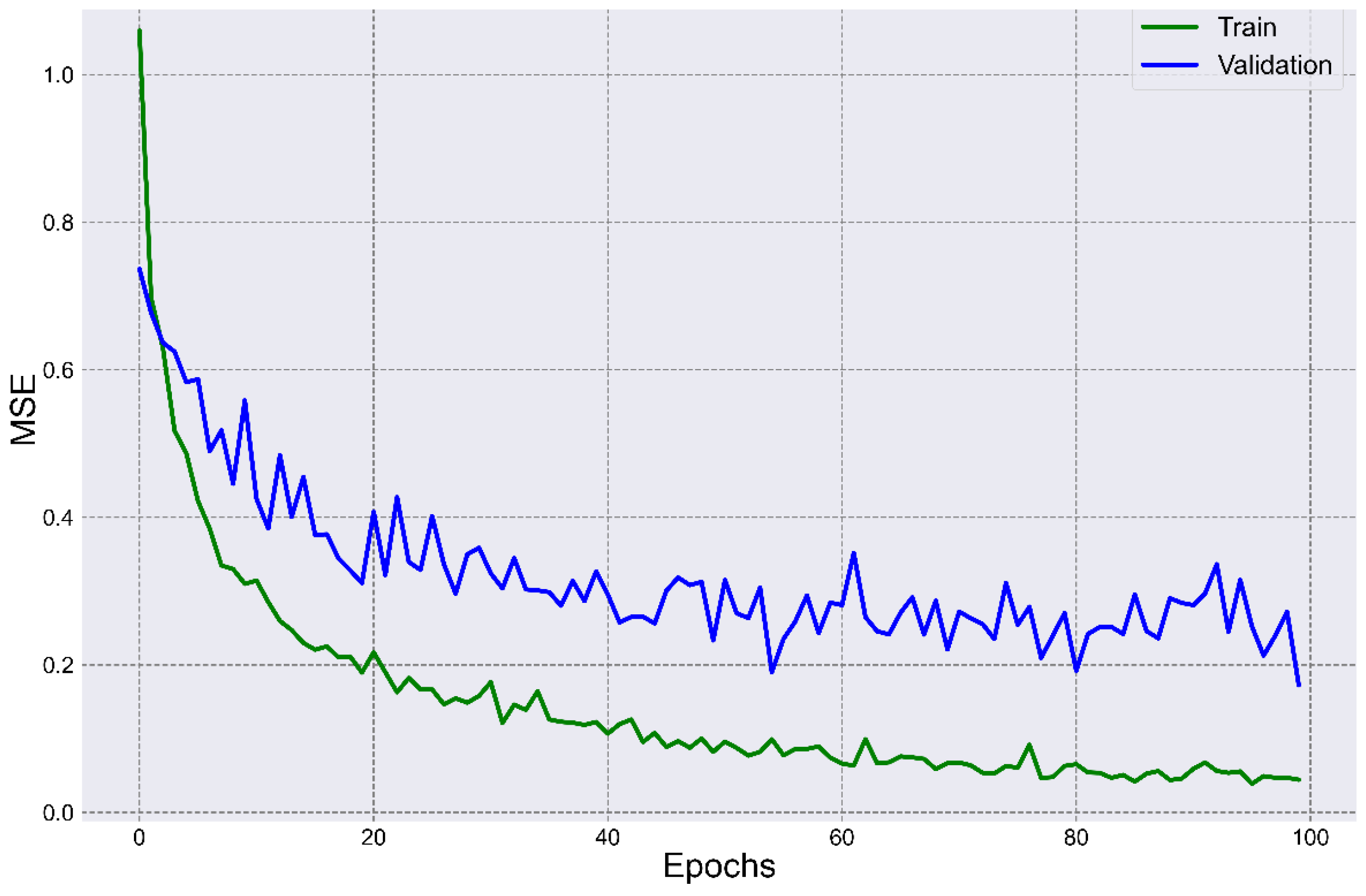
Figure 4 shows the comparison of the loss function results for the training and validation datasets. The maximum
MSE in the first epoch was: training set—1.0597; validation set—0.7914. The minimum
MSE in the 100th epoch were training set—0.0443 and validation set—0.1725.
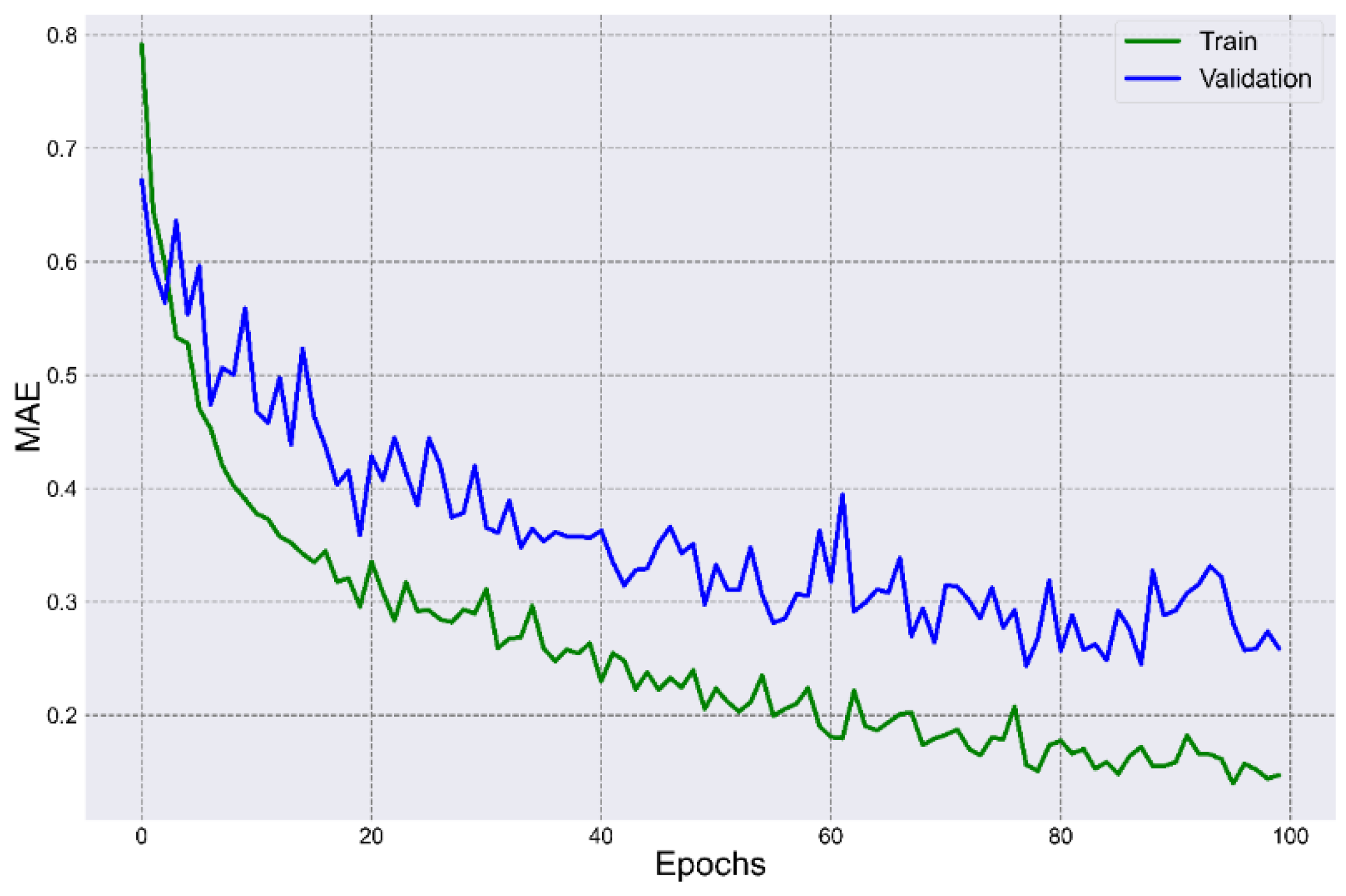
Figure 5 shows a comparison of the results of calculating the quality metric for the training and validation datasets. The maximum
MAE value in the first epoch was training set—0.7914 and validation set—0.6721. The minimum
MAE for the training set (0.1399) was reached in epoch 96 and the validation set (0.2439) in epoch 78.
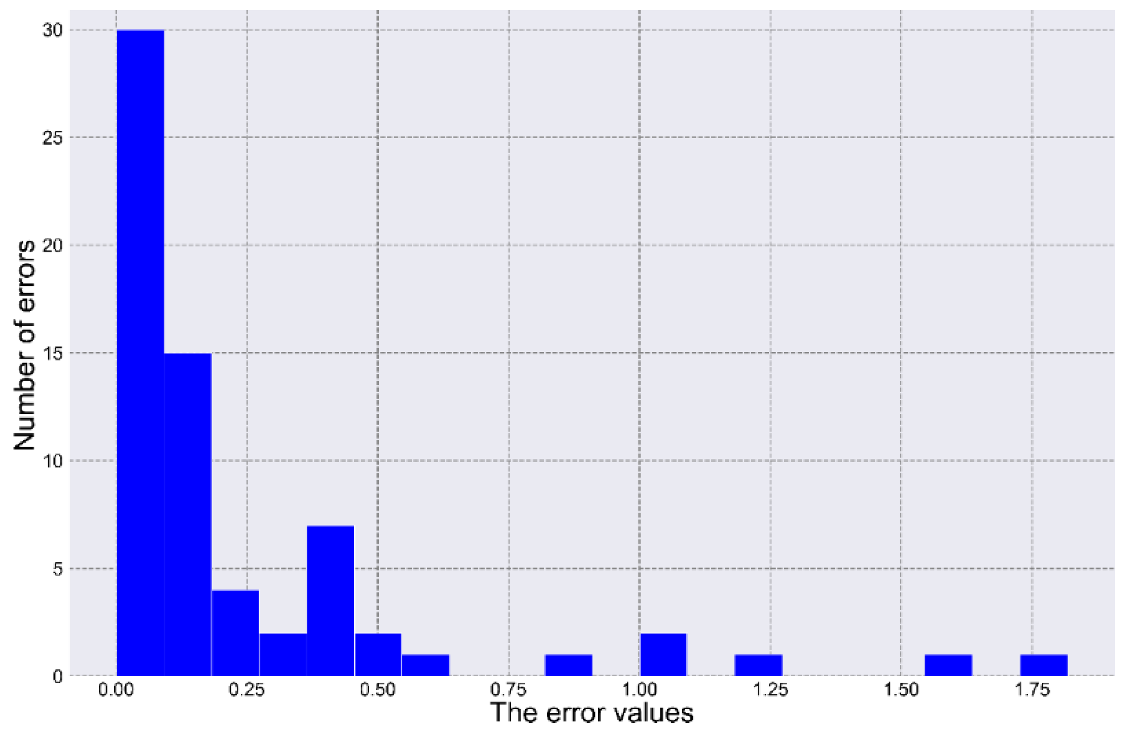
The histogram of errors (
Figure 6) shows that most of the errors fall within the range from 0 to 0.25, although there are some anomalous errors.
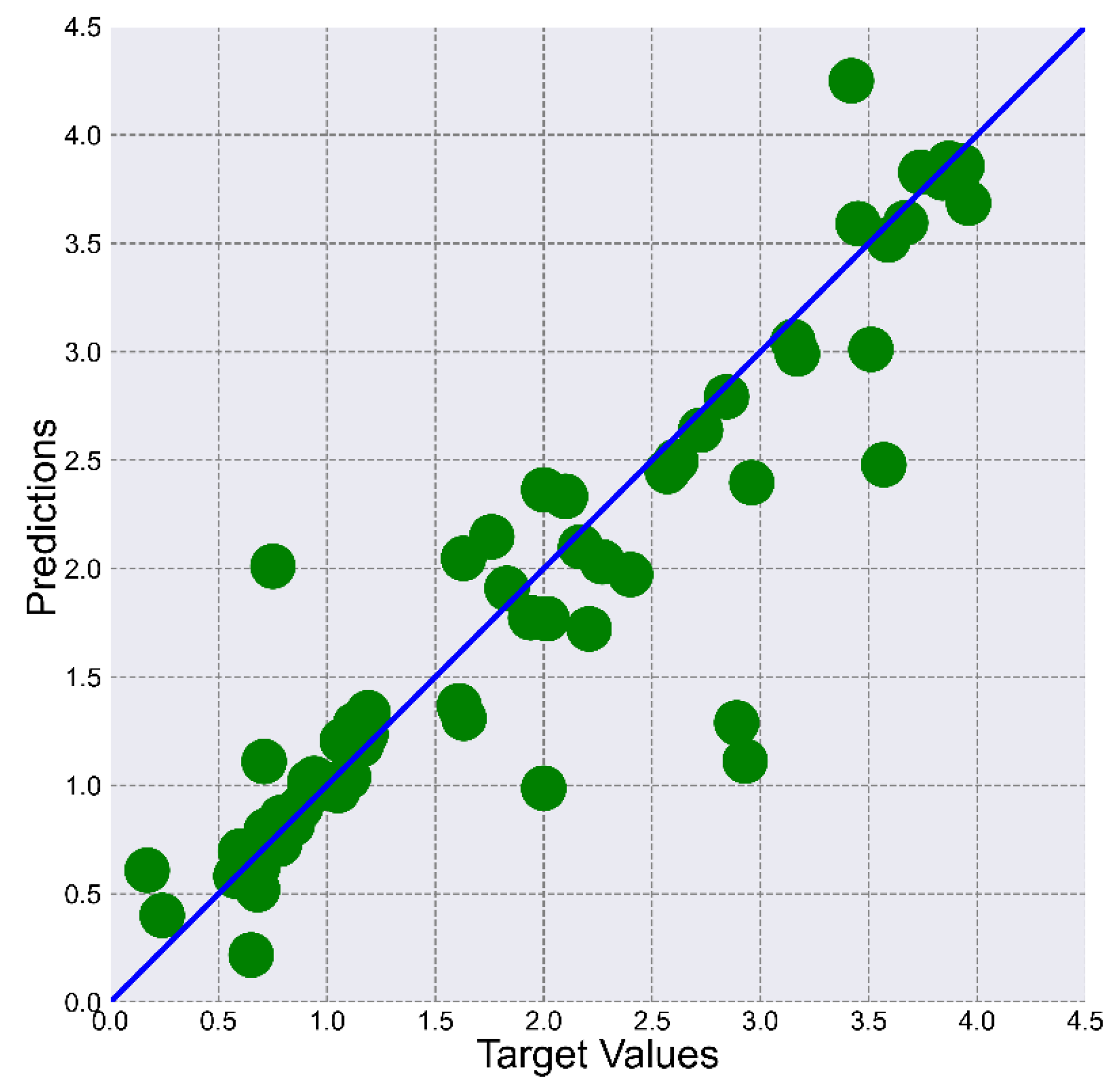
Figure 7 shows the scatter of the predicted values relative to the target values.
In general, the prediction values fit reasonably well against the target values, except for a few outliers. Most likely, there are significant anomalies in the output for these values that require data cleanup. The results of the R2 calculation also serve as indirect confirmation of the anomalies in the data. For example, there are input datasets whose R2 values are −4.73 and −1.60.
One of the main methods to analyze the ANN model is the comparison of various indicators (mean absolute percentage error,
MAPE; root mean square error,
RMSE; mean square error and
MSE), and the coefficients of determination (
R2) and regression (
R). Tijanić, Car-Pušić and Špera [
44] argued that
R2 and
MAPE are the most often applied estimators of the model accuracy. The authors set the goal of their study to predict the cost of road construction. The values of
R2 and
MAPE indicators were 0.959 and 13%, respectively. Mounter et al. [
45] investigated the capabilities of ANN to improve the accuracy of long-term predictions of building energy consumption. The
MAPE indicator was 12.03%. Kulisz et al. [
46] aimed to study ANN ability to model the water quality index in groundwater. They used the coefficient of determination (
R2 = 0.998) as a measure of ANN accuracy. Szul, Nęcka & Mathia [
47] used five different ANN to predict energy consumption. To assess the quality of the developed models, the
MAPE and
R2 indices were used, the values of which were 13.7% and 0.8, respectively. Ding et al. [
48] used the ANN model to predict the power output of a PV system. Their results showed 10.06% and 18.9%
MAPE forecast errors during sunny and rainy days, respectively.
Thus, comparing the MAPE and R2 indicators of the created ANN model (MAPE = 14.1%; R2 = 0.847) with other cases, it can be stated that, in general, the degree of agreement between the measured and modelled data is satisfactory.
The low level of the ANN model results (MAPE and R2) were associated with two causes. Firstly, the peculiar ability of limestone to increase pH values faster at lower doses. When limestone is added to water, such water becomes a complex dynamic system.
The water pH value is the ratio of H
+ to OH
−. The peculiarity of such a system is as follows:
The pH value increases due to CaCO3 dissolution. The peculiarity of the CaCO3 property is that its dissolution occurs up to a certain point. Then, a reverse process begins, which is the interaction of Ca2+ with CO32− and the formation of CaCO3. Secondly, the measurement of the values of water quality parameters (pH, Eh, TDS) was influenced by the permissible metrological errors of the measuring instruments.
Based on the data obtained, the authors believe that the created ANN can be used to achieve the study task and could later be applied to predict changes in the water pH value when adding various doses of limestone.


