Online System for Power Quality Operational Data Management in Frequency Monitoring Using Python and Grafana

Abstract

This article proposes a measurement solution designed to monitor the instantaneous frequency in power systems. It uses a data acquisition module and a GPS receiver for time stamping and traceability. A Python-based module receives data, computes the frequency, and finally transfers the measurement results to a database. The frequency is calculated with two different methods, which are compared in the article. The stored data is visualized using the Grafana platform, thus demonstrating its potential for comparing scientific data. The system as a whole constitutes an efficient, low-cost solution as a data acquisition system.

1. Introduction

The static and dynamic characterization of power systems is essential in order to assess the quality of the electricity supply (Power Quality, PQ). One of the most critical parameters is frequency, since its stability has a decisive influence on the operation of electrical machines. Special mention requires those that operate in synchronized mode, for which the deviations that occur with respect to their nominal value required for correct operation, are inadmissible [1].

As the characteristic parameters of the network can oscillate within a permitted range without being inappropriate for the equipment, it is essential to monitor whether they fall within these limits. In fact, in reality, the European frequency (50 Hz) is quite unstable, since the delivered signal is not perfectly sinusoidal, its admissible limits being 50 ± 0.1 Hz for systems with synchronous connection and 50 ± 2 Hz for isolated networks. [2,3,4].

Frequency shifts depend on a number of external factors. Common causes are lightning strikes, connection and disconnection of huge loads, nonlinear loads, and groundings or short circuits in transmission lines [2]. Some well-known solutions have been developed to track the frequency, based on multiple procedures, for instance Zero Crossing (ZC) methods, Quadratic Forms (QF), Demodulation, Discrete (Fast) Fourier Transform (DFFT) with Phase Compensation (PC), etc. [3].

However, in the modern and increasingly intelligent electrical network (smarter grid) there are numerous distributed resources that, although a priori independent, require synchronized monitoring in order to evaluate the mutual influence and the global effect of their connection in the network. In response to this need, ad hoc measurement equipment was developed, the most relevant being the phasor measurement units (PMUs) [5,6,7,8,9,10].

PMUs are used to estimate the magnitude and phase of electrical magnitudes (e.g., voltage or current) [6,7,8,9,10,11]. Synchronization features are provided via GPS or IEEE 1588 Precision Time Protocol (PTP), designed to allow real-time synchronization of several remote points in the grid. PMUs capture samples of the power line signal and rebuild the so-called phasor quantity (magnitude and phase), which constitutes the mathematical model of the waveform under test. The result is a time-synchronized measurement quantity known as syncrophasor [10,11].

PMUs are capable of detecting abnormal waveform shapes. For instance, if both supply and demand do not match perfectly, the associated frequency imbalances cause “tightness” within the grid, which is a potential cause for power outages. PMUs are also designed to measure the frequency in the power grid. Indeed, a typical commercial PMU can report measurements with very high temporal resolution, up to 120 measurements per second (30, 60 and 120 are common reporting rates) [10]. This helps with analyzing dynamic events in the grid, which is not possible with traditional SCADAs that generate one measurement every 2 or 4 s. Therefore, PMUs with enhanced monitoring and control capabilities are considered as one of the most important measuring devices in the current and future design of power systems [7,8,9,10,11,12].

Besides the high prices (the average overall cost per PMU—the cost for procurement, installation and commissioning—ranges from USD 40,000 to USD 180,000), in most cases PMUs measure the voltage magnitude and the phase angle, assuming that the frequency remains constant [6]. This starting hypothesis is precisely disregarded in PMU’s indirect measurements. These operations are essentially based on the formulation of a mathematical problem whose purpose is to fit the measurements to a sinusoidal curve. Consequently, when the sinusoidal curve is not ideal, the PMU fails to make exactly that adjustment. In this way, the less sinusoidal the voltage supply signal, the worse the adjustment made and the lower the quality of the phasor generated. This situation is very common in the modern grid, in which distributed and random generation, and the presence of nonlinear loads, make it necessary to adopt new strategies in order to complement the existing ones based on PMUs [13,14].

Considering all of the above, the present work proposes a monitoring solution for the frequency of the electrical network (grid frequency), which is complementary to the existing ones, based on PMUs, in the following double sense that constitutes the core essence of the contribution of this work. On the one hand, it provides a more precise frequency measure, based on the Allan variance, and thus contributes to the enhancement of the characterization of the network. On the other hand, the system is capable of managing large volumes of data (big data) that flood the electrical network [15], allowing the user to extract the necessary information at all times for a better and less subjective way of understanding the energy management and quality of the supply (PQ).

The instrument hardware is based on the GPS receiver-data acquisition (DAQ) system binomial; the latter driven by a computer program developed in Python. The first one provides traceable time stamping, with the help of the 1 pulse per second (PPS) signal, and a precision of 1 ppm. In this way, the developed system adapts to what is established in the PQ regulatory framework [2], obtaining frequency values every 10 s, with a temporal resolution better than 20 ms [5,6], minimizing delays associated with heavy software diagrams and programming codes.

Another proposal and challenge of the present work is the use of Grafana as a visualization tool for massive data related to the quality of the supply, and specifically to the frequency of the network. The work is part of an emerging trend of development of low-cost data acquisition frameworks, which often constitute alternative solutions and complementary functionalities to those offered by SCADAs [9]. Commercially named PyFreqDAQ, this DAQ-F system incorporates an easy-to-use graphical user interface, allowing a simple control and automation of a huge variety of experimental setups for frequency measurement.

This is the motivation of the work and the general context of the research. The rest of the paper is structured as follows. Section 2 provides details regarding the system description and arrangement. Then, in Section 3, PyFreqDAQ operation is detailed along with the frequency calculation. Section 4 displays and explains graphical results of data analysis from Grafana. Finally, conclusions are drawn in Section 5.

2. System Description and Arrangement

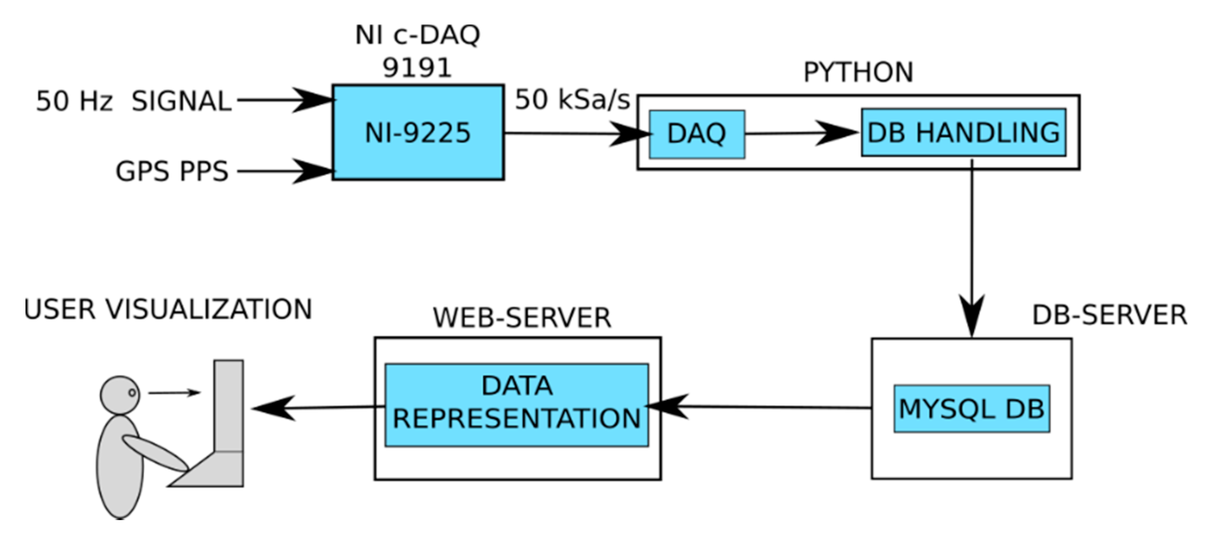
From here onwards, the proposed distributed instrument will be described. The hardware consists essentially of a chassis and a data acquisition card (DAQ) from the manufacturer NI™, which receives, on the one hand, the voltage input (50 Hz, 220 V_rms) from the electrical network and, on the other, the pulsed signal (1 PPS) from the GPS receiver (Symmetricon™) disciplined clock. The pulses of the latter are used as traceable references for time domain stamping and as references to calculate the frequency according to the Allan variance (Figure 1). The data are transferred from the acquisition card to the computer via Ethernet. Later, they are processed, and the processing results transferred to the database. All this is performed by software programmed in Python. Using these data, it is possible to graph the evolution of the frequency in the required time interval, in order to carry out the monitoring of the electrical network [13].

The monitoring solution developed according to this strategy allows for obtaining data from multiple measurement sources, and putting them in common in a database, which is available on the display. With this, since a large amount of signal data from different points can be observed and analyzed (compared), the maintenance of the network can be carried out using spatial and temporal compression strategies, which offer a simplified and truthful statistical vision of the huge amount of initial data (big data).

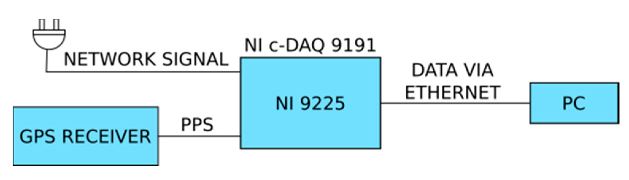
In order to obtain an overview of the measurement solution, Figure 1 shows a block diagram, which indicates the direction of the signal flow and the interactions between the different elements that make up the system.

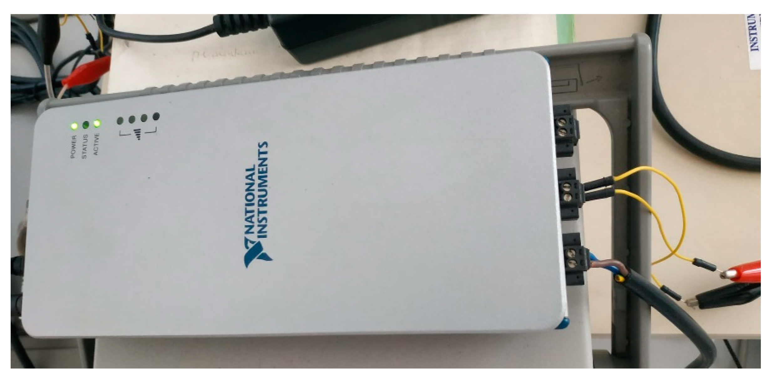
The PyFreqDAQ measurement chain consists of a GPS receiver for the synchronization, a plug connected to the network responsible for acquiring the signal, and a DAQ card that receives both signals and sends them to the PC. This can be seen in detail in Figure 2.

Figure 3 shows the connections of the GPS-PPS and the voltage signals to the card NI 9225 (simultaneous, channel-to-channel isolated). This three-channel module allows up to 300 V_rms, with a sampling frequency of 50 kS/s and 24 bits. Data are used to calculate frequency later. The card NI 9225 is allocated inside the chassis NI 9191. The chassis controls timing, synchronization and data transfer between I/O modules and the external server.

The equipment, model Symmetricom™ TrueTime XL-AK GPS synchronized receiver, assures ultraprecise time and frequency delivery. This configurable piece of instrument provides timing outputs within 40 ns of UTC/USNO and frequency outputs accurate to less than 1 × 10⁻¹². It includes 1 PPS output that provides a reference for the frequency calculation using the Allan variance.

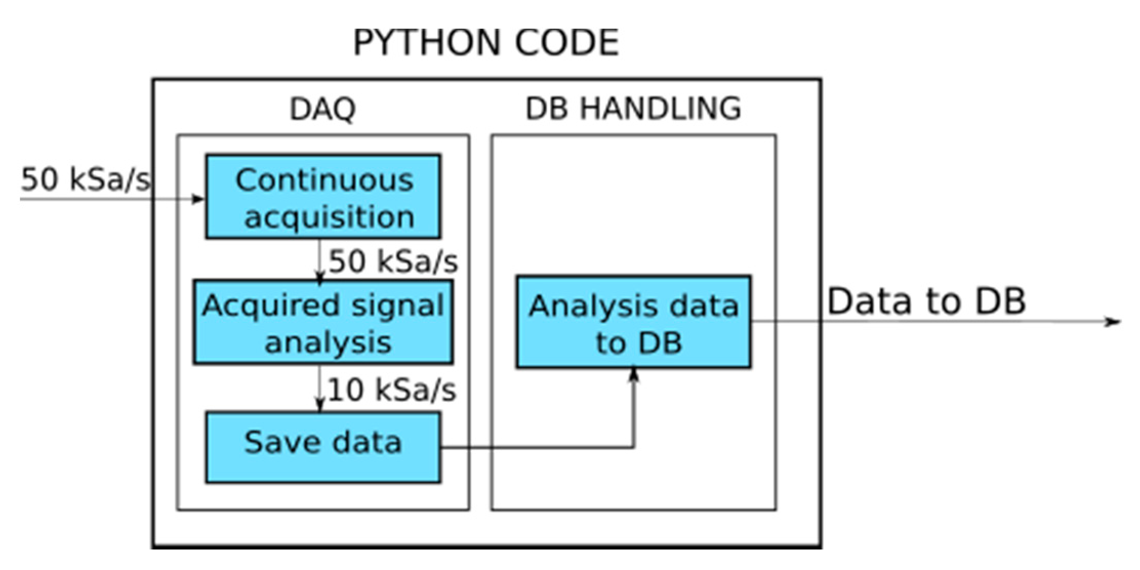
For data processing, calculations, as well as sending information to the database, two Python software projects are constantly running in parallel. The first one is responsible for receiving data transmitted from the NI 9225, calculating frequency and sending the results to the second one. First project is referred to as “DAQ”; the second project being responsible for receiving data from the DAQ and organizing it within the database. This part is referred to as “DB handling”. 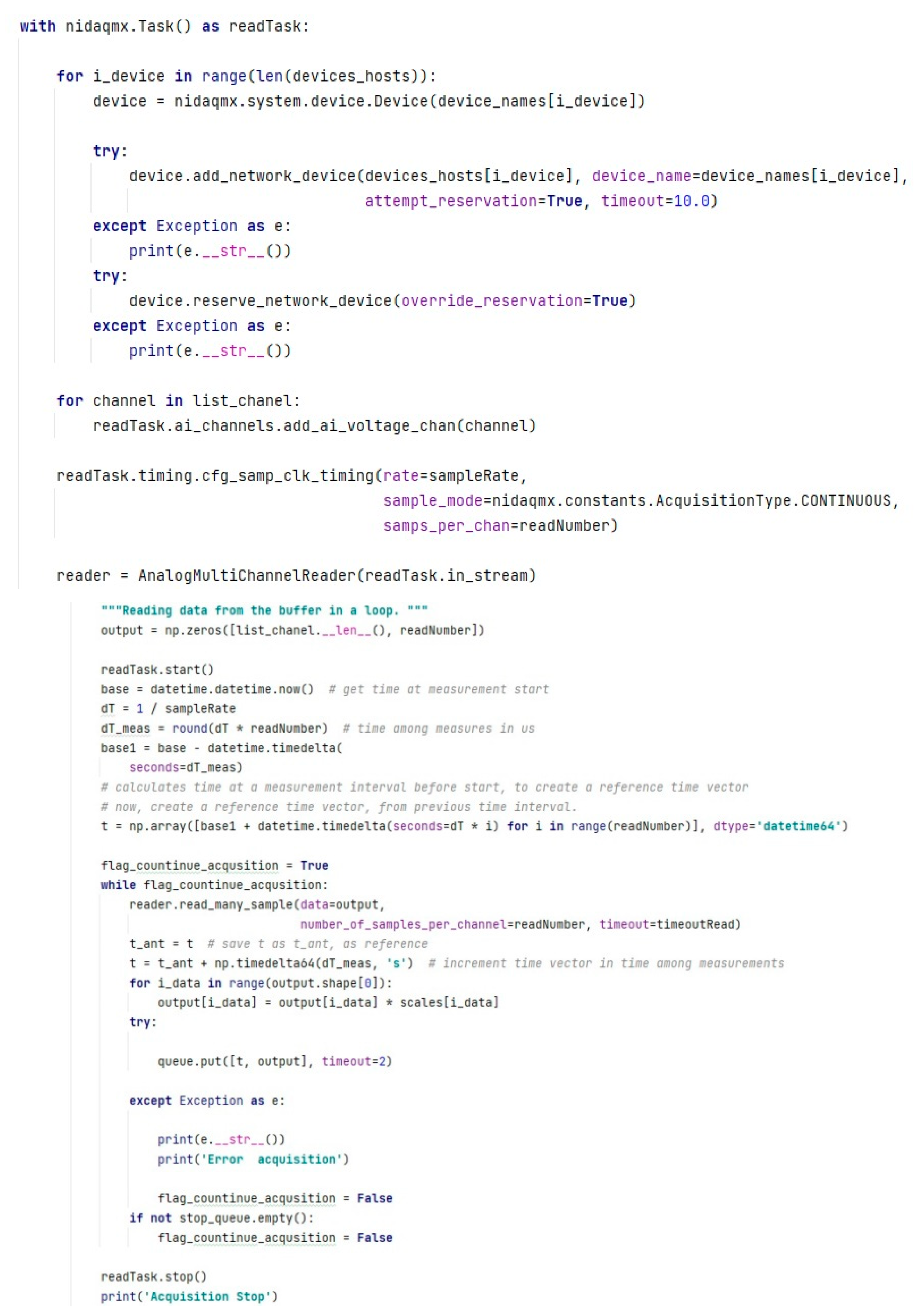Figure 4 shows, in a simplified way, the workflow of the projects, and Figure 5 shows the Python codes associated with data acquisition.

Finally, data is represented on Grafana, a well-known, multiplatform, open-source analytics and interactive visualization web application. It provides charts, graphs, and alerts for the web when connected to supported data sources. As a visualization tool, Grafana is a very popular component in monitoring stacks, often used in combination with time series databases and monitoring platforms. In this work, it allows for user data surveillance.

3. PyFreqDAQ Operation and Frequency Calculation

The card NI 9225 receives data from two inputs (sampling frequency is 50 kS/s): the voltage line signal by connecting directly to a wall plug, and the GPS-PPS signal that allows an absolute time reference. Raw data are then transferred via Ethernet to the software running on the PC.

The first of the two projects, referred to as “DAQ”, is constantly reading signal data acquired from the NI 9225. Calculations are performed in two ways. The PPS is used for the calculations contemplating the theoretical frequency of 50 Hz, so each theoretical cycle lasts 20 ms.

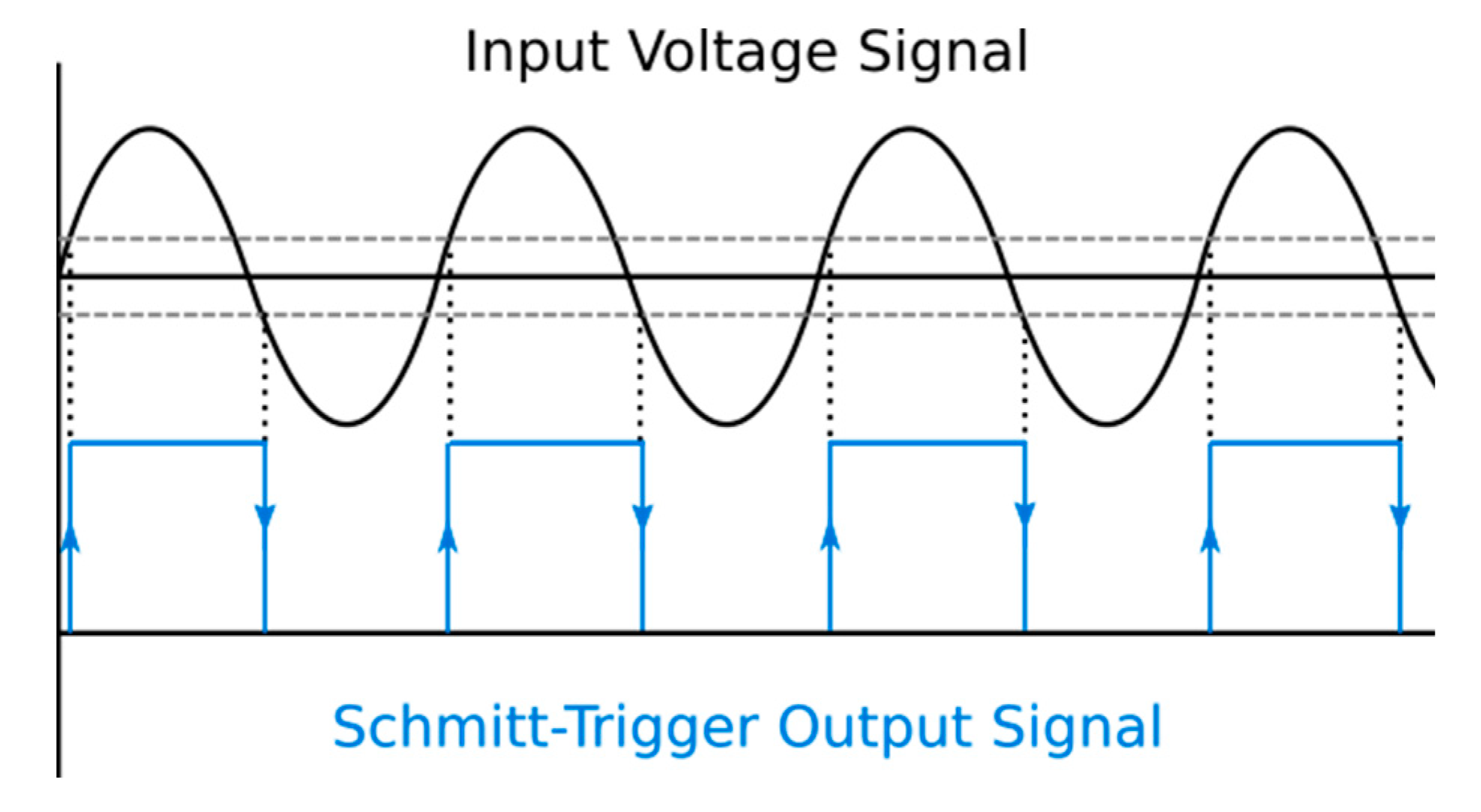
The voltage line is driven to a Schmitt trigger in order to be conditioned (it returns a square waveform with the same frequency as the input signal). When the input voltage is higher than a chosen upper threshold, the output is high, and when the input falls below a lower level, the output is low. If the input voltage is between both thresholds, the output remains in the same previous state (Figure 6). Then, calculations can be performed by fragmenting this square waveform into its cycles.

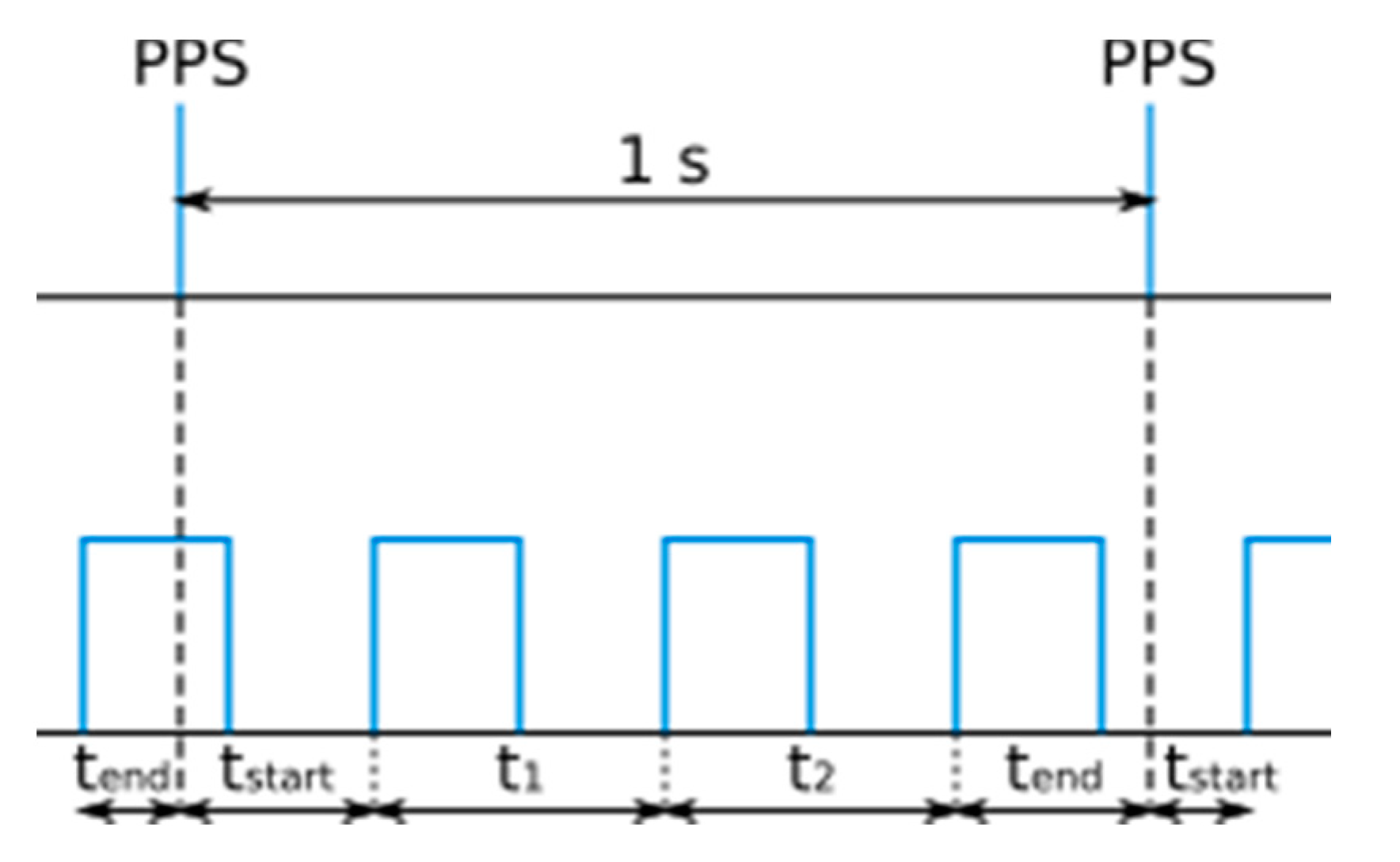
Between every two pulses coming from the GPS (1 PPS signal), complete periods of the signal boxed by the Schmitt-trigger can be found, as well as part of them, which have been interrupted by the 1 PPS signal. The sum of all of them must be equal to one second. Figure 7 shows an example of this circumstance that shows the exact behavior of the signal processing.

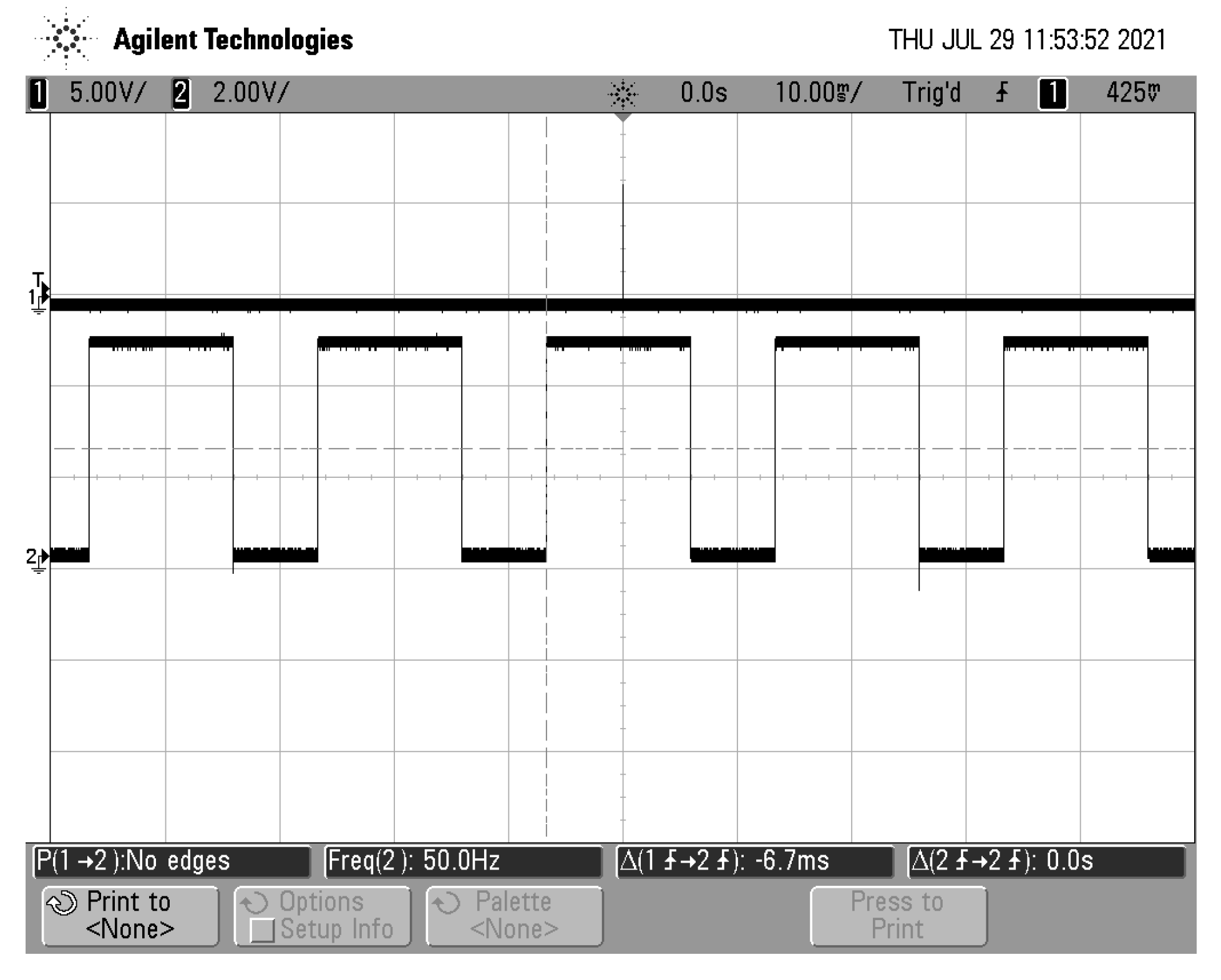
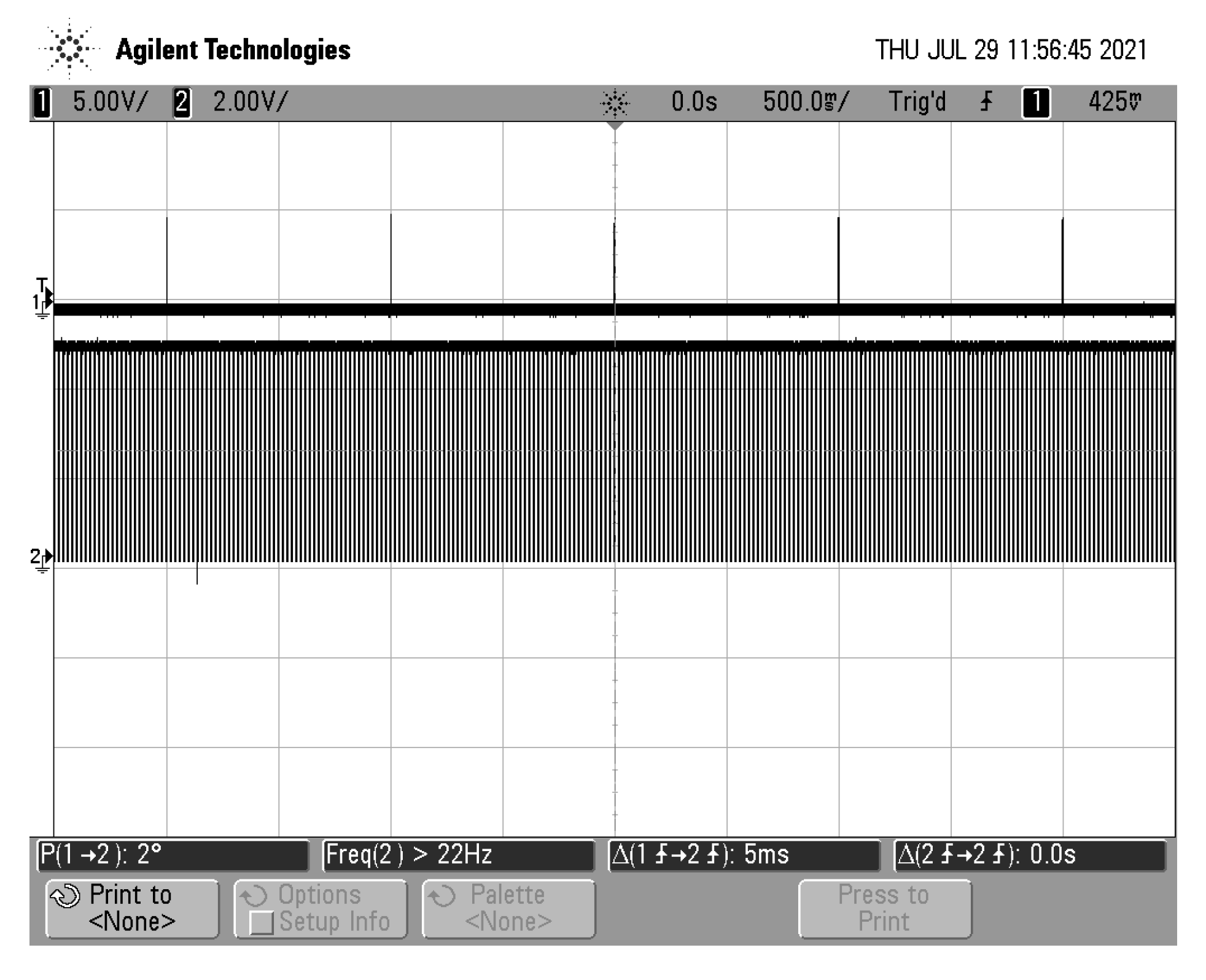
For those cycles that contain a GPS-PPS signal, the phase is measured, bearing in mind that each cycle corresponds to a phase shift of 360°. The next two illustrations, Figure 8 and Figure 9, show the real PPS signal from the GPS receiver and Schmitt-trigger signals, at different sampling rates, from the lab oscilloscope.

Using the signal phase, hereinafter Allan variance is calculated. It has exhibited efficient performance in frequency stability characterization of precision sources in authors’ previous works [13]. Furthermore, frequency. The first parameter to be considered in the computation scheme is known using the Allan variance, we can calculate frequency using frequency deviation from a reference as the fractional frequency deviation:

$$\mathrm{y}\left(\mathrm{t}\right)=\frac{\mathrm{f}\left(\mathrm{t}\right)-{\mathrm{f}}_0}{{\mathrm{f}}_0}$$

(1)

This depends on the actual frequency and the base frequency, f₀. In this case, f₀ corresponds to the ideal network frequency of 50 Hz. It is calculated by the deviation from the actual frequency with respect to f₀, in a relative or fractional form.

Time deviation is also calculated, starting from the base frequency. At an instant t, the signal advances a phase of ϕ(t). If the frequency was equal to the base one:

$$\mathsf{\varphi }\left(\mathrm{t}\right)=2\mathsf{\pi }{\mathrm{f}}_0\mathrm{t}$$

(2)

So, if ϕ(t) is divided by 2π${\mathrm{f}}_0$, and the frequency is ideal, it would result “t”. Then, if we subtract “t” from that fraction, time deviation can be obtained for an instant t but also instant t + 1:

$$\mathrm{x}\left(\mathrm{t}\right)=\frac{\mathsf{\varphi }\left(\mathrm{t}\right)}{{2\mathsf{\pi }\mathrm{f}}_0}-\mathrm{t}$$

(3)

So far, as each increment of +1 corresponds to an increment of τ in time, it can be determined as a fractional time increment, which would be equal to the frequency increment:

$$\begin{gathered} {\overline{\mathrm{y}}}_{\mathrm{k}}=\frac{1}{\mathsf{\tau }}\left({\mathrm{x}}_{\mathrm{k}+1}{-\mathrm{x}}_{\mathrm{k}}\right) \\ =\frac{1}{\mathsf{\tau }}\left(\left(\frac{{\mathsf{\varphi }}_{\mathrm{k}+1}}{2\mathsf{\pi }{\mathrm{f}}_0}-\mathrm{t}\left(\mathrm{k}+1\right)\right)-\left(\frac{{\mathsf{\varphi }}_{\mathrm{k}}}{2\mathsf{\pi }{\mathrm{f}}_0}-\mathrm{t}\left(\mathrm{k}\right)\right)\right) \\ =\frac{1}{\mathsf{\tau }}\left(\frac{{\mathsf{\varphi }}_{\mathrm{k}+1}-{\mathsf{\varphi }}_{\mathrm{k}}}{2\mathsf{\pi }{\mathrm{f}}_0}-\mathrm{t}\left(\mathrm{k}+1\right)+\mathrm{t}\left(\mathrm{k}\right)\right)=\frac{1}{\mathsf{\tau }}\left(\frac{\Delta \mathsf{\varphi }}{2\mathsf{\pi }{\mathrm{f}}_0}-\mathsf{\tau }\right) \end{gathered}$$

(4)

The phase increment is computed using the start and ending phases, before and after the PPS signal:

$${\mathsf{\varphi }}_{\mathrm{end}}=2\mathsf{\pi }·\frac{{\mathrm{t}}_{\mathrm{end}}}{{\mathrm{t}}_{\mathrm{start}}{+\mathrm{t}}_{\mathrm{end}}}$$

(5)

$${\mathsf{\varphi }}_{\mathrm{start}}=2\mathsf{\pi }·\frac{{\mathrm{t}}_{\mathrm{start}}}{{\mathrm{t}}_{\mathrm{start}}{+\mathrm{t}}_{\mathrm{end}}}$$

(6)

Additionally, with them, the phase increment of each second is:

$$\Delta \mathsf{\varphi }={\mathsf{\varphi }}_{\mathrm{start}}+2\mathsf{\pi }\mathrm{N}+{\mathsf{\varphi }}_{\mathrm{end}},$$

(7)

N being the number of cycles. All in all, the instantaneous frequency at instant t for the kth-measure obeys the following equation:

$$\frac{{ \overline{\mathrm{f}}}_{\mathrm{k}}}{{\mathrm{f}}_0}{-1=\overline{\mathrm{y}}}_{\mathrm{k}}; \frac{{\overline{\mathrm{f}}}_{\mathrm{k}}}{{\mathrm{f}}_0}{=\overline{\mathrm{y}}}_{\mathrm{k}}{+1; \overline{\mathrm{f}}}_{\mathrm{k}}{=\mathrm{f}}_0\left({\overline{\mathrm{y}}}_{\mathrm{k}}+1\right)$$

(8)

Expression of ${\overline{\mathrm{y}}}_{\mathrm{k}}$ from Equation (4) is replaced in Equation (8):

$${\overline{\mathrm{f}}}_{\mathrm{k}}{=\mathrm{f}}_0(\frac{1}{\mathsf{\tau }}\left(\frac{\Delta \mathsf{\varphi }}{{2\mathsf{\pi }\mathrm{f}}_0}-\mathsf{\tau }\right)+1)$$

(9)

If $\mathsf{\tau }$ = 1, we have:

$${\overline{\mathrm{f}}}_{\mathrm{k}}{=\mathrm{f}}_0(\frac{1}{1}\left(\frac{\Delta \mathsf{\varphi }}{2\mathsf{\pi }{\mathrm{f}}_0}-1\right){+1)=\mathrm{f}}_0\frac{\Delta \mathsf{\varphi }}{2\mathsf{\pi }{\mathrm{f}}_0}=\frac{\Delta \mathsf{\varphi }}{2\mathsf{\pi }}$$

(10)

$\Delta \mathsf{\varphi }$ is then replaced using Equation (7):

$${\overline{\mathrm{f}}}_{\mathrm{k}}=\frac{{\mathsf{\varphi }}_{{\mathrm{start}}_{\mathrm{ant}}}+2\mathsf{\pi }\mathrm{N}+{\mathsf{\varphi }}_{\mathrm{end}}}{2\mathsf{\pi }}$$

(11)

Splitting into simple fractions and replacing ${\mathsf{\varphi }}_{\mathrm{start}}$ and ${\mathsf{\varphi }}_{\mathrm{end}}$ by their expressions in Equations (5) and (6) yields:

$${\overline{\mathrm{f}}}_{\mathrm{k}}=\frac{{\mathrm{t}}_{{\mathrm{start}}_{\mathrm{ant}}}}{{\mathrm{t}}_{{\mathrm{start}}_{\mathrm{ant}}}+{\mathrm{t}}_{{\mathrm{end}}_{\mathrm{ant}}}}+\mathrm{N}+\frac{{\mathrm{t}}_{\mathrm{end}}}{{\mathrm{t}}_{\mathrm{start}}{+\mathrm{t}}_{\mathrm{end}}}$$

(12)

As is observed in Figure 6, ${\mathrm{t}}_{\mathrm{start}}$ is the time elapsed from the initial PPS to the end of the cycle which is broken by this pulse, and ${\mathrm{t}}_{\mathrm{end}}$ is the time elapsed from the beginning of the last cycle (considered between the two PPS) and the final PPS.

The frequency is calculated according to two different methods. On the one hand, a specific method is used in which the frequency and its associated uncertainty are calculated every second using the method based on Allan variance. On the other hand, a traditional method has been used, regulated in accordance with the UNE 50160 standard, which calculates the frequency every 10 s.

Once the calculations are performed, data results are transferred to the second Python project (DB handling). This project is responsible for saving and organizing MySQL database, with the aim of being rapid. Grafana obtains data directly from the database and represents it with timescales and other resources so that the user can visualize the evolution of the variables.

4. Results

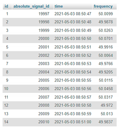
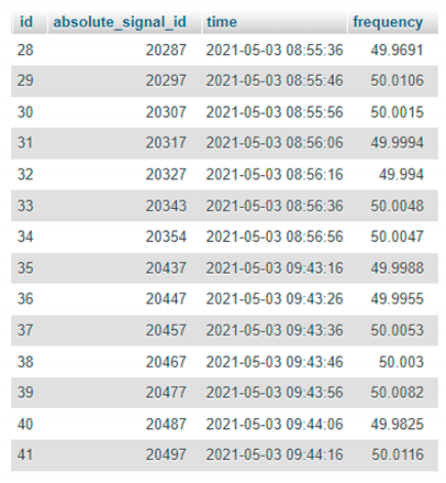
The database is organized according to different tables. If necessary, the information could be stored in the same table, but this would lead to very heavy data matrices, which would slow down the search engine, and consequently all the operations derived from it would entail a high computational cost. To emphasize this size, putting the focus on the Allan frequency, which is the most loading case of the two measurement strategies compared in this work, one result is sent to the database every second, resulting in 86,400 rows generated per day; 604,800 per week; in one month, 18,748,800 and in one year 31,536,000. To solve the above-mentioned big-data issues, this is programmed directly by the DB handling, for both Allan and regulated frequencies. As examples,

Table 1. Allan frequency table (offline measurements) for one month, extracted from Grafana database. It keeps its original format.

and

Table 2. Frequency measurements (according to norm 6100-4-30) table extracted from Grafana.

show the measurements corresponding to the month of May. Each table preserves its original design in order to show a Grafana perspective.

It can be verified that one frequency datapoint has been generated each second just looking at the “time” column.

Additionally, it can be verified that frequency is registered in 10-second periods, as is stated. In both tables there are four columns, labeled: “id”, “absolute signal id”, “time” and “frequency”. “id”: primary key of the correspondent table, autoincrement, serves to enumerate the rows of the monthly table. “Absolute signal id”: foreign key from the global signal list table. “Time”: date in which the measurement was taken. Format: YYYY-MM-DD HH:MM:SS. “Frequency”: calculated frequency value in Hz. Following these critera, it is faster to make the queries that are aligned with Grafana. Indeed, Grafana uses data stored in tables for implementing the desired graphics. The graphics are called “Dashboards” and the users can create as many as desired using available data [15].

The platform is capable of selecting data from the tables according to certain search criterion. For example, in the present work, for the sake of representing the evolution over time of frequency values, the table of a specific month for a specific time interval to be represented can be selected. In this case, the platform extracts only the columns of time and frequency from the tables.

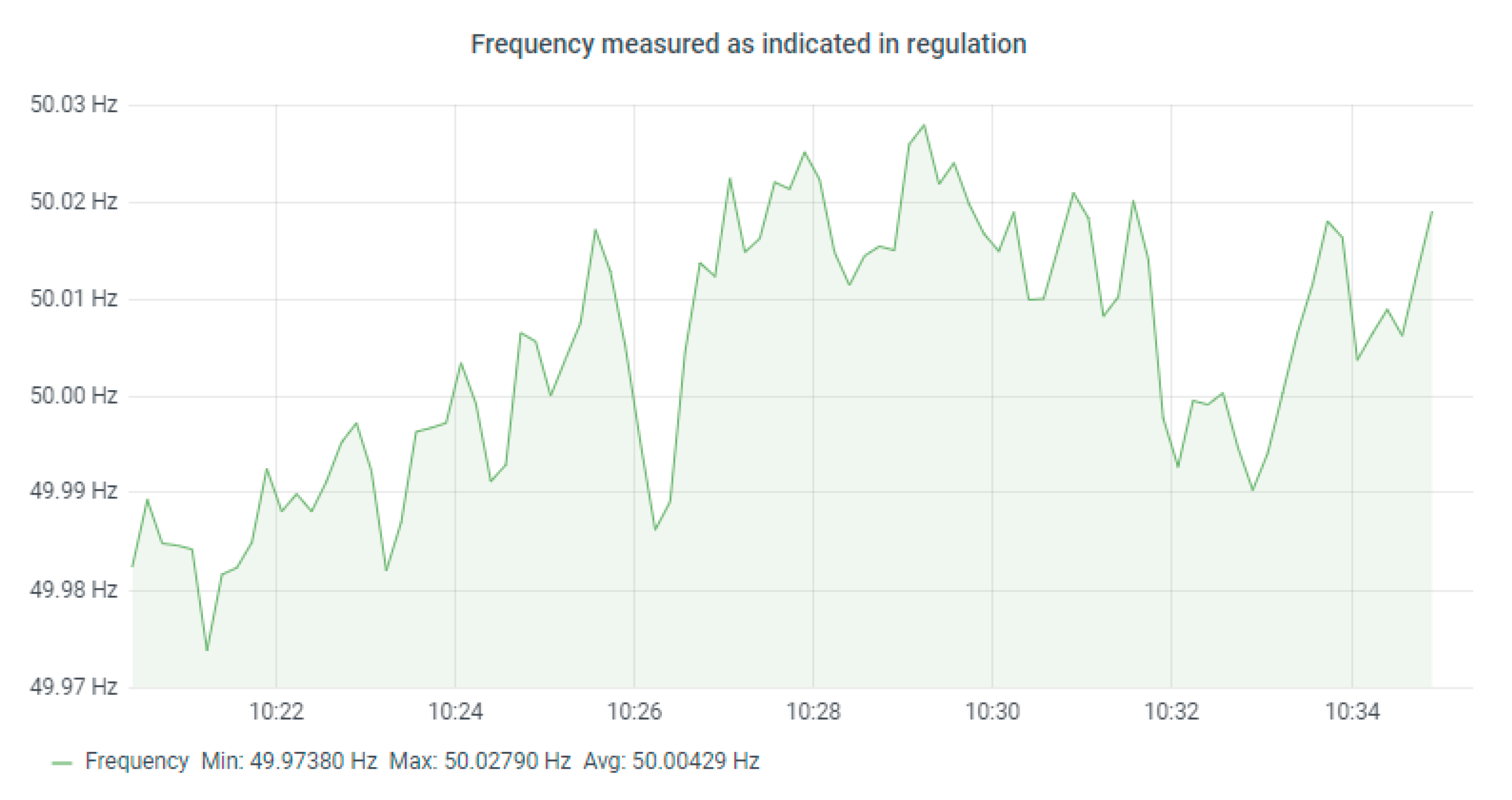
The standard UNE-EN 50160:2011 establishes the limits that the frequency cannot overtake, and mentions that the frequency has to be measured using 10-s periods [2]. Figure 10 shows the evolution of the frequency over 15 min, measured as indicated by the norm.

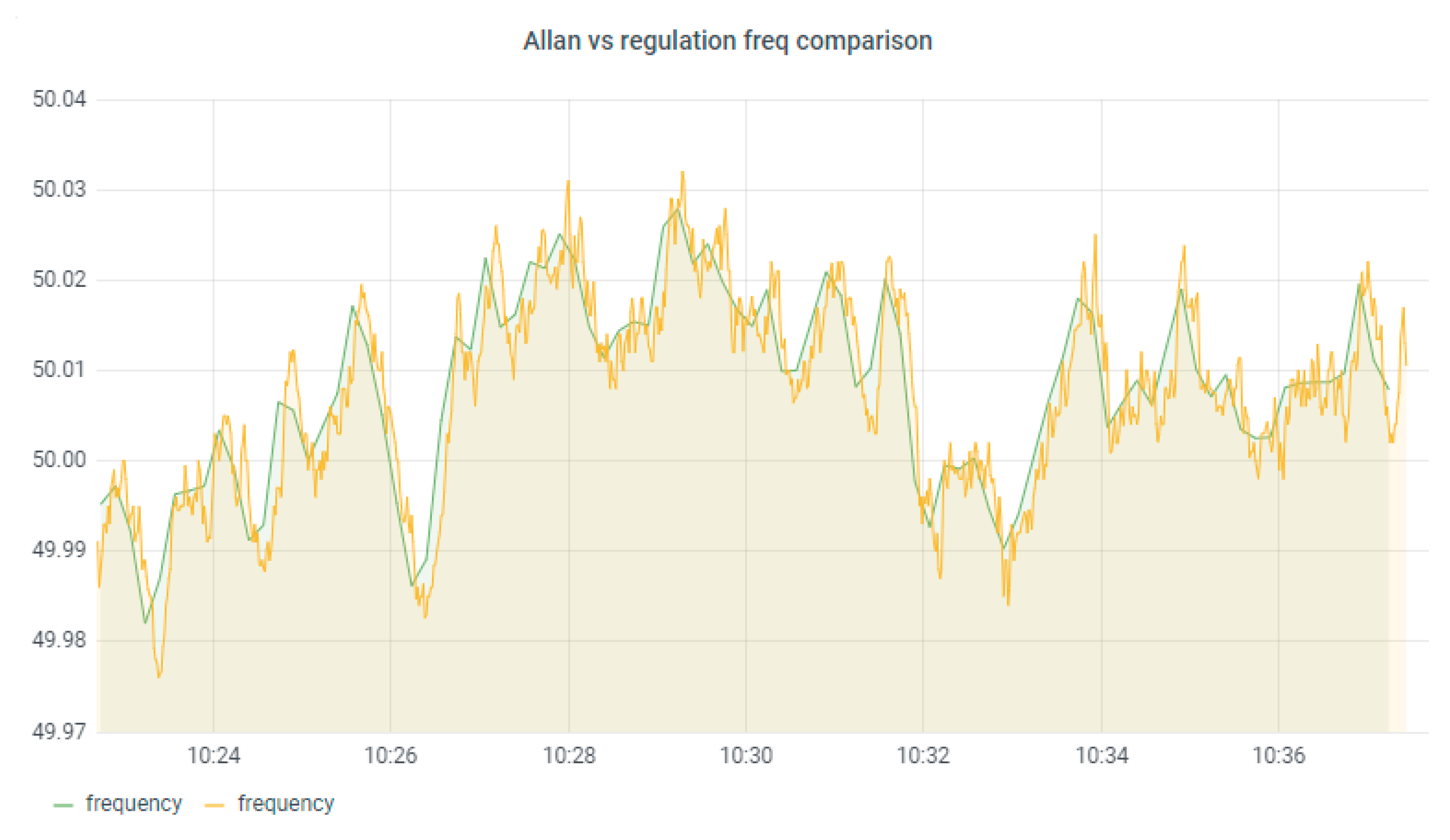
To study the difference between the two frequency calculation methods, the following dashboard on Grafana compares the evolution of both frequencies. A time interval of 15 min has been chosen, as can be observed in Figure 11.

Looking at Figure 11, the difference between the results the two methods is clear. First, the evolution of frequency measured by the regulation method looks softer than the other one. The reason is clear; with the method that establishes the regulation, the frequency calculation is conducted for periods of 10 s, so one measure is available for each 10 s. With the Allan algorithm, frequency is calculated each second, so the number of measures available is 10 times greater, thus there is a tendency for a lot of peaks compared to the other one.

In addition to this, Allan frequency is totally synchronized thanks to the GPS-PPS signal, so it can be stated that this method is more accurate that the one that regulation establishes.

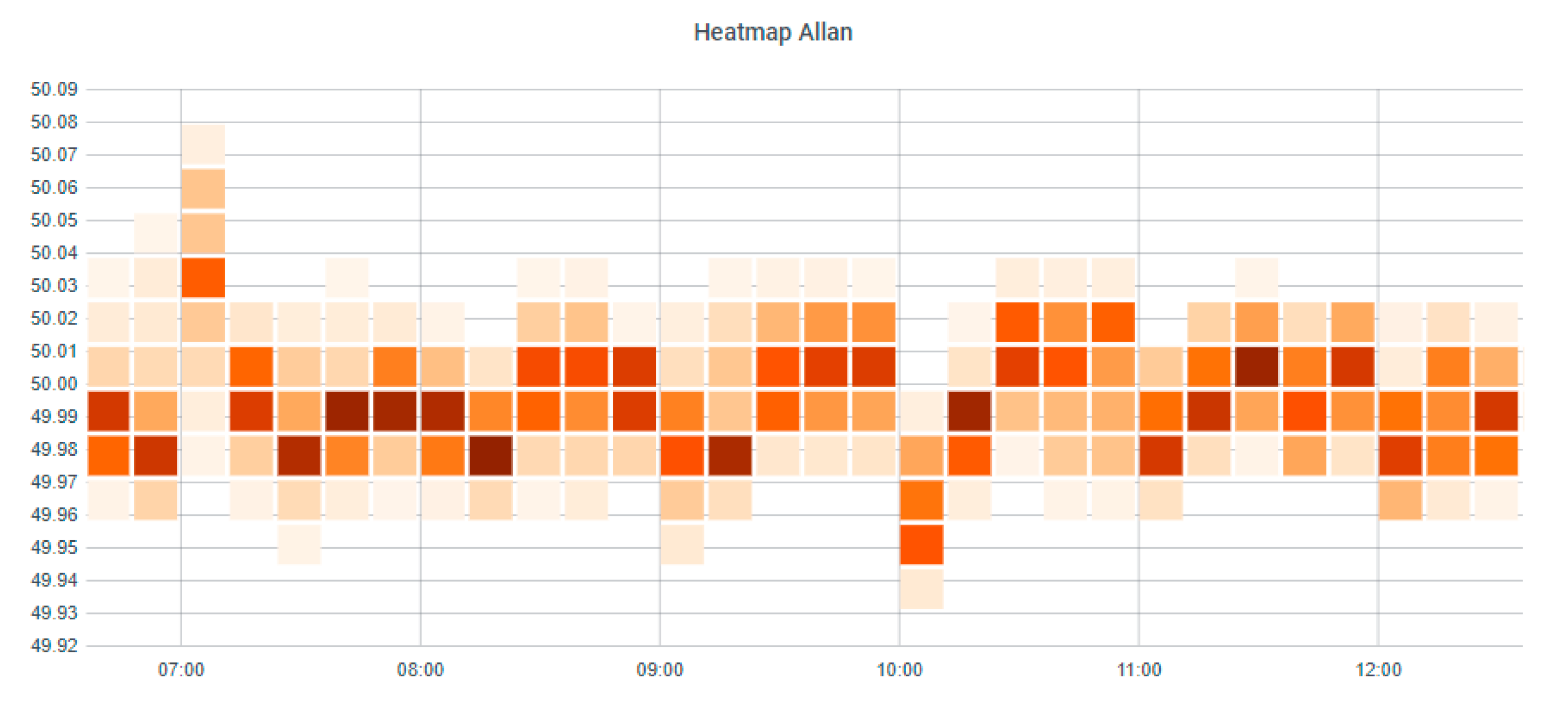
Observing the measures over time, it has been proven that frequency did not exceeded the established limits for at least 10 s, in which case, frequency would be out of what current regulation dictates. A Grafana a heat-map showing the distribution of Allan frequency through time is also presented (Figure 12).

The horizontal axis corresponds to the timescale. Figure 12 is divided into one-hour intervals. Each interval contains five columns of squares, so each column corresponds to an interval of twelve minutes. The vertical axis corresponds to the frequency scale. As the Allan frequency is measured each second and each square in column corresponds to twelve minutes, for each column we have 720 measurements. To indicate the distribution of these measurements, in each column there are various squares of different colors. The darker the square, the more measurements have been recorded within the considered frequency interval. It can be observed that data continuously fluctuate around 50 Hz. The rest of the measurements are assumed to be outliers, as observed in fluctuations that fall outside the frequency range of 49.95–50.03 Hz, approximately.

5. Conclusions and Future Work

In this work, a low-cost measurement solution (called PyFreqDAQ) has been proposed to monitor the frequency of the electrical network, considered as a quality parameter of the electrical supply, and at the same time offer a more precise result thanks to the use of the Allan variance. The hardware is managed by Python, and open-source software (Grafana) is available that allows for monitoring the evolution of the frequency, in order to study the limits between which it is maintained. This measurement solution is original in that it does not use high-level visual programming software for data acquisition and data management (e.g., labVIEW™), thus lightening the computational load, an issue that could be the subject of future work.

In order to show its operating power, the frequency has been calculated according to two different methods. The first is in accordance with the regulations of the IEC 61000-4-30 standard. The second uses an algorithm that provides the measured frequency with greater precision and a reference traceable via GPS, which is the Allan variance-based algorithm.

Among the many benefits of the Allan variance-based method it is worth citing its better precision, lower error, faster calculations, and a wider range of measurements available to users.

The use of Python to program the data acquisition card and manipulate the database has shown much greater flexibility than other applications (e.g., labVIEW™). In effect, Python is a more powerful programming language, and consequently, it allows operations and calculations to be carried out using simple codes, while allowing for a low computational load and consuming much less working memory. In future works, a Python vs. labVIEW™ comparative could be studied, which would be unique research, to date.

All in all, the joint use of Python and Grafana to receive and process, perform operations on and visualize the data, has proven to be very efficient in the sense of perfectly adapting to the regulations and at the same time offering a flexible measurement solution, which is adapt to the modern and smart electrical grid.

Finally, the emerging Grafana monitoring solution in the field of distributed instrumentation, not considered to date in power-supply quality studies, allows for a much easier visualization of the data within a web environment. In future works, the performance of Grafana against other web programming environments should be compared for a monitored variable, which could be the frequency of the network or the industrial frequency. Research could look at comparing computation times, flexibility and ease of choice of the variables to be displayed. Indeed, with Grafana and the measurement platform developed by simply choosing a set of parameters and connecting them to the database, the visualization is interactive and immediate, constituting a simple task that requires little time, that can be carried out by an operator plant with a very basic training.