Abstract
This article contains a review of essential control techniques for maximum power point tracking (MPPT) to be applied in photovoltaic (PV) panel systems. These devices are distinguished by their capability to transform solar energy into electricity without emissions. Nevertheless, the efficiency can be enhanced provided that a suitable MPPT algorithm is well designed to obtain the maximum performance. From the analyzed MPPT algorithms, four different types were chosen for an experimental evaluation over a commercial PV system linked to a boost converter. As the reference that corresponds to the maximum power is depended on the irradiation and temperature, an artificial neural network (ANN) was used as a reference generator where a high accuracy was achieved based on real data. This was used as a tool for the implementation of sliding mode controller (SMC), fuzzy logic controller (FLC) and model predictive control (MPC). The outcomes allowed different conclusions where each controller has different advantages and disadvantages depending on the various factors related to hardware and software.
1. Introduction
The International Plant Protection Convention predicted in 2021 a possible climate scenario for 2050 in which the global surface temperature will increase between 1.5 C and 2 C unless deep reductions of CO are achieved in the following decades [1]. Based on the latest report conducted by the international energy agency, this would imply that renewable energies should cover at least 70%, where the half is expected to be supplied by wind and sun [2]. There is an implication that we will use PV systems, one of the fastest growing industries of renewable energies in recent years [3]. Benefits are related to null emissions, avoidance of mechanical moving parts, and no generation of noise during its operation [4].
A PV system is composed of several solar cells made of semiconductor materials where the role of these is to absorb photons to generate an electron-hole pair through a p-n junction [5]. This action, which exposes an electron diffusion to produce voltage, is a complex process since not all the solar light spectrum is possible to be captured [6]. Actually, this effect induces a PV conversion efficiency that tends to be lower than 20% [7].
Solar cell technologies consider semiconductor materials such as types of crystalline, such as polycrystalline Silicon (poly-Si) and thin film type which are frequently produced from cadmium telluride (CdTe) or copper indium gallium selenide (CIGS). The CdTe’s major feature is its chemically stable composition which provides different production methods where the most popular at the moment is thin PV films [8]. The CIGS is capable of providing a long-term reliability in terms of their degradation [9]. Silicon solar cells can reach the highest among the three types which is around 15% [10]. Considerable advances in efficiency improvement allowed the invention of Interdigitated back contact (IBC) n-type solar cells which reported a value up to 24.4% [11]. However, IBC cells present a complex and expensive production method due to its novelty [12]. Not only the efficiency of PV systems can be low but also, the end-user voltage is unstable and depends on the light intensity [13].
A DC-DC converter can be linked to a PV to adjust the output voltage and current in a suitable operating point [14]. As reported by Raghavendra et al. [15], there are two main categories, which are isolated and non-isolated. The first mentioned refers to an electrical limit (such as a transformer) amid the inputs and outputs which allows the usage for high voltages. Examples of these types are flyback, forward, resonant, push-pull and bridge [16,17,18,19,20]. In the non-isolated, the configuration indicates that the mentioned barrier is vanished and therefore, the efficiency tends to be higher since the number of components is lower [21]. Known non-isolated architectures are Cuk, SEPIC, boost, buck-boost, positive superlift Luo, and ultra-lift Luo [22,23,24,25,26,27].
Since a PV setup has a low efficiency, the MPPT is an essential step because it helps the system to achieve the best overall performance [28]. This can be generated through a designed control technique that can be embedded in a DC-DC converter [29]. Therefore, in this paper, a revision of different MPPT for photovoltaic systems techniques are examined. Despite that, several authors provided reviews about MPPT methods for PV systems [30,31,32], a major contribution of this work is the implementation of four of the revised algorithms in a real platform in combination with a neural reference generator. In regards to the PV test rig, because the solar panel had a low output-voltage, it increased with a boost converter that is known for this main feature [33].
The article is summarized as follows. Section 2 contains the analysis of different MPPT techniques with their advantages and disadvantages, Section 3 shows the implementation of selected algorithms in a real PV rig which details are explained, Section 4 exhibits the obtained results during the experiments and Section 6 concludes with the major outcomes of this study.
2. Overview of MPPT Control Strategies
In 1954, a group of scientists from Bell Laboratories patented the first commercial solar cells with an efficiency of 6% [34,35]. Therefore in the same year, the MPPT was the objective of researchers to increase the efficiency and enhance the performance of this invention [36]. Another involved reason was that the electricity produced by the PV system which changes along the time as the position of the sun is variable. Furthermore, the electricity produced by the PV system is dependent on solar light (irradiance) and environmental temperature [37]. Thus, it becomes a significant challenge to harvest the MPPT of a PV system [38].
Figure 1 summarizes the algorithms that had been highlighted in this review. Mainly there are two types of MPPT trackers: mechanical and electrical [36]. In regards to the first type mentioned, which is also known as a “solar tracker”, it can increase the energy production up to more than 40% on average [39]. Nevertheless, this configuration is recommended for industrial applications rather than for domestics due to the excessive cost involved of the mechanical tracking devices [40].
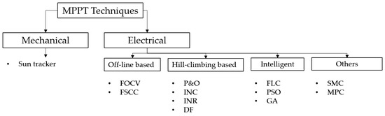
Figure 1.
Overview of the analyzed methods in this article.
On the other hand, electrical MPPT techniques are dependant on the power-voltage and linked to current-voltage curves to track the optimal operative point [41]. Conventional curves for a PV system are revealed in Figure 2 where the nonlinear feature is showed. Additionally, the MPP increases its complexity when the temperature, irradiation and partial shadowing vary to produce different curves with alternative shapes [42,43,44]. Therefore, to force a PV system to work at the MPP, many algorithms were introduced by the researchers.
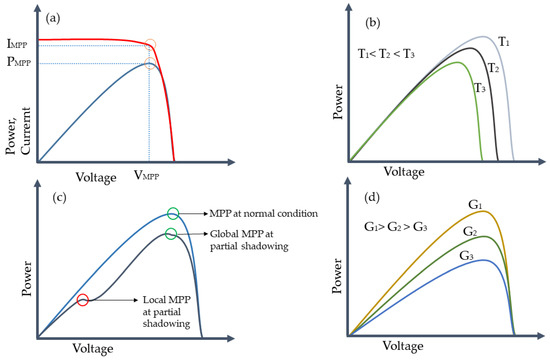
Figure 2.
Typical curves for a PV system where: (a) is a conventional power-voltage and power-current graph with the MPP highlighted; (b) shows how the power-voltage curves change with different temperature at constant irradiation; (c) displays the change due to partial shadowing in power-voltage curves; (d) exhibits the variation of the power-voltage curves with constant temperature and variable irradiation.
2.1. Offline Techniques
Known offline calculation algorithms advantages are related to their simplicity to be embedded and low computational demand [45]. The mechanism is based on constant linear approximations to achieve the MPP. Fractional open-circuit voltage (FOCV) belongs to this group and focuses on the MPP through a proportional relation between the MPP voltage () and the open circuit voltage () [46]. A similar approach is fractional short-circuit current (FSCC), which as its name suggests, it is related to a relation between the current at the MPP () and the short circuit current () [47]. The accuracy of these methods is highly dependant on the proportional constant in which the FSCC has on a vastly with greater inaccuracies for MPPT [48].
The FOCV method was implemented in experiments by Frezzetti et al. [49] for a PV system. In this research, the authors used an adaptive scheme based on the irradiation to achieve acceptable results. FSCC has also been used in real time for a PV system based on the research made by Sher et al. [50]. In the latter, a hybrid scheme linked to a P&O even-thought that the efficiency was lower than the conventional P&O.
2.2. Hill-Climbing Algorithms
Hill climbing (HC)-based algorithms are widely employed in research and industry due to their high efficiency with low computational requirements [51]. These methods have the ability of avoiding the usage of empirical data for voltage and/or current tracking. Therefore, it is possible to achieve the MPP without a former knowledge of the PV features [45]. The principle of HC is schematically explained through Figure 3 where the slope calculation between power and voltage would give an idea about the position on the graph and thus, an action to be taken such as increasing or decreasing the voltage. In this section, main hill climbing algorithms like perturbation and observation (P&O), incremental conductance (INC), incremental resistance (INR), and drift-free (DF) are reviewed.
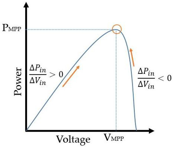
Figure 3.
Principle of the hill climbing algorithms for MPPT.
2.2.1. Perturb and Observation
This algorithm is based on an intentional and periodical perturbation on the control command with a following observation and evaluation of the system output [52]. Applied to PV systems, the perturbation is generated through a change in the voltage and current , such that the power of the PV is measured. This implies that the slope can be calculated, which helps with knowing whether the MPP is achieved, as Figure 4 shows.
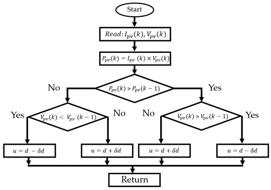
Figure 4.
Flowchart of P&O algorithm.
Based on the previous description and on the detailed logic of Figure 4, the knowledge of and and its delay in allows for the calculation of the slope. Therefore, if the latter mentioned value is positive, the duty cycle d will increase such that the algorithm output and aims to reach the MPP; on the contrary, when the position is at the right side of the MPP, the control signal decreases through .
An interesting example of simulated implementation of P&O was carried out by Murtaza et al. [53], where they used this algorithm for a two-stage coordinated PV system. Despite that this study lacks of experimental results, the authors showed that it is also effective in distributed systems. Another case where experiments were involved in a PV system showed that conventional P&O techniques are very sensitive to step size (which is related to the disadvantages of this method) [51].
Despite the fact that P&O is one of the most popular MPPT algorithm in industry due to its simplicity [54,55]. Regardless of these assets, the major downsides are high chattering when the MPP is reached and the lack of success to achieve this point [56]. The latter are majorly related to the changes in temperature and solar irradiance [57].
2.2.2. Incremental Conductance
The incremental conductance technique is widely used for MPPT applications because it has higher accuracy in comparison to P&O. The calculation of the incremental change in conductance by evaluating the effect of voltage change [58]. The conventional INC uses the slope of the P–V curve [59]. The slope P–V curve at MPP is zero; the slope is positive when MPP is on the right side and negative when MPP is on the left side. The controller injects a slight change in the duty cycle and observes the behavior of the conductance [60]. This algorithm was implemented in experimental conditions by authors of [61], where they provided a regulated step size routine and the results showed a suitable performance. Disadvantages related to this scheme are reported to the trade-off between the system dynamics and the steady state accuracy that is managed within the controller tuning [62]. The flowchart of the whole algorithm is shown in Figure 5.
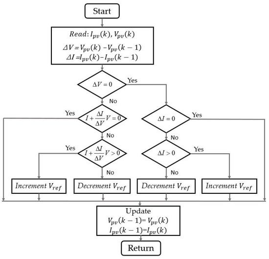
Figure 5.
Flowchart of INC algorithm.
2.2.3. Incremental Resistance
Previously described algorithms worked in the power-voltage curve but alternatively, INR employs the power-current to determine the sign of the following perturbation [63]. Differently to INC, the evaluation in this case is through the current change. Research by Raedani and Hanif conducted experimental implementation [64]. The authors found that the convergence is slower than P&O and INC. The reported downsides of this method are related to the associated scaling factor for the change of reference voltage which can be complex to accomplish [65]. A descriptive flow mechanism of this tool is displayed in Figure 6.
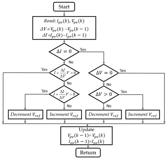
Figure 6.
Flowchart of INR algorithm.
2.2.4. Drift-Free
If a sudden change in irradiation occurs with any of the previous algorithms, it can happen that the new operative point lies on the opposite side of the MPP. For instance, an operative point that is in the left side of the MPP (based on a power-voltage curve), it can switch to the right side due to an irradiation change or likewise for the opposite situation. This effect is known a drift which can be harsh if large step-sizes are used [63]. Nevertheless, Kili et al. [66] proposed a modified P&O algorithm to overcome the drift where the mechanics is based on the addition of a new parameter that figures if the power change is produced by intentional (due to algorithm) or by irradiance. The procedure of this algorithm is explained in Figure 7. A basic experiment carried by Mathew et al. was found where they used a drift-free algorithm [67]. The authors found that the algorithm behaved better than INC under changing operative conditions.
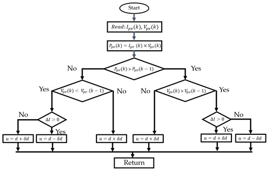
Figure 7.
Flowchart of Drift-free algorithm.
In regards to the advantages, this algorithm can deal with unexpected irradiance variations with high efficiency in terms of the lost power [68]. Nevertheless, the downsides occur when the load varies since it is ignored. A solution for this problem was proposed by Jately et al. [63], although the algorithm and number of variables are higher.
2.3. Intelligent Techniques
Intelligent techniques are aimed to provide high performance in comparison to previous described ones. In this sense, the features are related to fast responses, overshoot avoidance and low fluctuations in irradiance or temperature changes so that the operative point can stay at the MPP [69]. In this section, the algorithms to be revised are fuzzy logic control (FLC), particle swarm optimization (PSO) and genetic algorithm (GA).
2.3.1. Fuzzy Logic Control
FLC is based on the human experience rather than knowledge of the system’s mathematical model [70]. In this review paper, type-1 fuzzy (which structure is displayed in Figure 8) sets are revised which mechanism comprises a fuzzification, an inference and a defuzzification block [71]. The fuzzification role is to map the inputs to a fuzzy variable [72]. Later the inference block is where the real data from an expert takes places through membership rules within if-then statements [73]. Finally, the output takes places in a defuzzification process where the linguistic rules of the inference are translated into numerical crisp values [74].
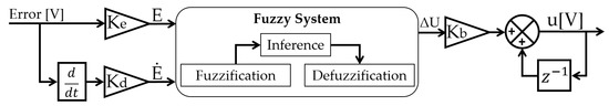
Figure 8.
FLC Structure.
The authors of [75] showed (through a simulation case) that FLC combined with P&O is capable of dealing with drifting. In real-time systems, Bakkar et al. made an implementation in a commercial PV [76]. In this case, they used a commercial PV with a flyback converter, commonly employed for low power applications [77]. Results of this experiment showed that the stability and fast response could be achieved.
The mentioned features of FLC allows concluding that a main advantage of this approach is that a mathematical model is unnecessary for the control tuning since it can be based on trial and error made by the designer [78]. Disadvantages are dependant on the available computational resources since the requirements will be higher as long as the number of rules are higher [79]. An example of this is with adaptive neuro-fuzzy inference system (ANFIS) which is a fuzzy approach based on neural networks [80]. In this latter, an improved simulation results were obtained for an MPPT approach in a PV system. Nevertheless, the computational costs are too high for implementation in real-systems [81].
2.3.2. Particle Swarm Optimisation
This stochastic method was developed on basis of the biological behavior of fish and bird flocks during travel when they are seeking food [82]. The animals are represented by multiple particles that are looking for a suitable path while they exchange information about the search among themselves [31]. Therefore, each particle position converges to a particular solution for a right path which are all evaluated and the best particle experience () within the best global one () [83]. Equations (3) and (4) are the mathematical representation for the velocity and position of each particle where and are the cognition coefficients to accelerate the particles to the suitable paths [84]. The parameter is called the inertia weight whereas and are arbitrary variables that belong in the range [0, 1] [85].
In the case of a PV system, the particle position is considered to be the duty cycle of the DC-DC converter and the velocity is the duty-cycle change [86]. The PSO algorithm is used for solving complex problems and optimization through a simple procedure that achieves high speed convergence [87]. However, one of the main issues is related to the high probabilities to fall in a local optimal point [88]. Additionally, the implementation in real time systems is complex since optimization algorithms require high computation time [89]. A particular solution can be through offline tuning in a high fidelity model. Al-Majidi et al. [90] provided this solution with a neural model trained with experimental data. Parameters were obtained through PSO and later an experimental test was configured to confirm the reliability of the strategy.
2.3.3. Genetic Algorithm
Based on Darwin’s natural principle, GA mechanics choose random potential solutions within a compatibility criterion [91]. This heuristic search method chooses a random generation for the creation of a later one and each is concerned with a fitness value [92]. There are two main operators for this case where the first one is the selection, in which the procedure is to pick the best chromosomes (bad ones are neglected) that will propagate a forward generation. The following operator is the reproduction that chooses two chromosomes from an ongoing generation to obtain individual for a future generation [93].
The mathematical mechanics are described in Equations (5) and (6), where an objective function is has constraints till the total number m as shown and a modification of this function defined as [94]. The constant K penalises the influence the following generation. As an example, the integral of the absolute error (IAE) can be a suitable objective function for MPPT [95].
The GA is capable of avoiding being stuck in local MPP as it works with condition which can be related to this condition [96]. This implies that it is able to work under a partial shadowing condition [97]. Nevertheless, this algorithm requires a huge amount of computational resources due to the iterative and constrained calculation [98]. This can also be mirrored at hardware implementation as in Attarmoghaddam et al. [99] where they only implemented one GA module.
2.4. Other Techniques
In this section, additional techniques are summarized. The structures described in this section are sliding mode control (SMC), which is as a robust controller widely used in uncertain systems, and model predictive control (MPC), as a prediction-optimization scheme. Since an error is involved in these schemes, the explanations were based on current tracking to achieve the MPPT. The error is defined in Equation (7) where and are MPP current and the PV output current, respectively.
2.4.1. Sliding Mode Control
SMC belongs to a robust control category since it is capable of dealing with parameter uncertainties, the design is simple and it has finite time convergence [100,101,102]. Based on Kihal et al. [103], three steps are necessary to achieve a suitable design:
- Selection of a surface for the sliding motion.
- Control Law design.
- Guarantee the reaching condition.
Equation (8) is the surface used for the following explanation. It is a proportional-integral surface that should accomplish with the Hurtwitz condition to guarantee that the error tends to zero when the system reaches a null value surface [104]. The parameter is a design value that should be tuned during experiments.
The control signal of a SMC is composed of an equivalent and a switching term , which are established in Equation (9). The first mentioned is achieved based on the condition [28]; the switching, which guarantees robustness, is expressed in Equation (10).
Based on the DC-DC boost converter model that was used in previous research [105], obtaining the equivalent control signal implies that the surface derivative should be equal to zero. Therefore, as the error was formerly expressed in Equation (7), and with the usage of the system (gathered from the authors previous work [24], the equivalent control term is achieved as follows.
In the experimental field, this method was tested in PV systems by authors of [106]. In this research, the authors implemented a SMC on a distributed MPPT that belonged to an electrical grid. Outcomes showed a proper accomplishment of the MPP with a correct control signal to avoid the system damaging.
Despite the mentioned advantages at the beginning of this section, disadvantages of SMC are related mainly to the switching feature of this method. Chattering is one of the most well-known disadvantages and it is caused because the switching is finite in real systems and due to unmodeled dynamics [107]. This effect not only increases the energy consumption of the system but also the actuators detriment [108].
2.4.2. Model Predictive Control
MPC is a method of constrained control that is based on the principles of feedback structures and numerical optimization [109]. Through the usage of a system that is capable of capturing the involved dynamics, MPC uses this tool to predict future states and select an optimized control action that can accomplish a determined performance index and defined constraints [110].
For this case, a discrete state-space model of the boost converter is obtained by means of the forward Euler approximation [111] given in Equation (12). Therefore, the discrete-time state-space model of the boost converter can be written as Equation (13).
The designed MPC seeks for the error minimization among the predicted current value and the desired reference. The future path of the states is achieved by the established dynamical system which are controlled through the prediction horizon. In this case, it was settled at a value of 2. The usage of Equations (14) and (15) allows the calculation of the controlled variable at each time . Thus, a cost function is associated with this objective which can be achieved through the numerical reduction of J, expressed in Equation (16). Since the authors applied an MPC in previous works, further mathematical details can be found in [112].
In terms of implementation, it was found that this method was implemented for a PV grid system by authors of [113]. They used an MPC, which was contrasted against a PID and outcomes displayed an increment of performance even during the appearance of disturbances.
MPC advantages are related to its robustness because it is capable of dealing with constraints and uncertainties [114]. Additionally, as it depends on a mathematical system, it is an intuitive method [115]. Nevertheless, since several operations are being performed at the same time such as optimization and prediction, this method is very sensitive to time parameters (like prediction horizon) because it can increase dramatically the computational time [116].
2.5. A Brief Resume of the Reviewed Techniques
Previous analysis settled to conclude a brief summary of MPPT techniques. The assets and weaknesses of each structure of the mentioned frameworks are concise in the following Table 1. Nevertheless, extra details were obtained in the following sections where experiments were performed in a real PV system.

Table 1.
Summary of advantages and disadvantages of the analyzed MPPT algorithms.
3. Experimental Case Study
In this section, four different MPPT algorithms were implemented and studied in a real PV system. The selection of the algorithms was based on the review previously made. In this sense, from the HC techniques, we selected the most used one that is P&O) which was compared with FLC, SMC, and MPC. Offline was not considered to be sufficient as non-linearities were expected during the experiments. Since SMC and MPC required a reference current/voltage that corresponded to the MPP, this was obtained via different techniques of previous works [117,118,119,120,121,122,123]. However, most of these approaches have a lack of accuracy which results in a low tracking efficiency. In this work an artificial neural network (ANN) was designed to obtain the reference current that corresponded to the MPP. First, different structures such as feed forward (FF), radial basis (RB), deep FF, etc., were tested to obtain an accurate prediction of . However, a recurrent neural network (RNN) was finally selected since it provided high accuracy for both training and validation performance.
3.1. Hardware Description
The hardware workflow involved in the experiments is shown in Figure 9. The PV panel was a commercial type manufactured particularly for residential and small industrial installations. The technical information of this device is listed in Table 2. Regarding the power converter, a DC-DC high step up type TEP-192 manufactured by the research group of Huelva University (Spain) was used. This hardware is an adaptation stage circuit that is inserted between the load and the PV generator. It is usually desired not only for boosting the PV low voltage, but also to provide regulated output voltage for end use. The characteristics of the device used in this work are provided in Table 3. To test the performance of the controllers, a programmable load resistance type 8500B manufactured by BK Precision Corporation (Yorba Linda, CA, USA) was used. The technical specifications of this device are listed in Table 4. A MicroLabBox dSPACE DS1202 (DT Techsolutions Pte Ltd., Singapore CITY, Singapore) also was used for the acquisition and control signal generation. This device has various channels for the communication with the host PC and the converter. The configuration of these channels can be made via its real-time-interface libraries. Additional equipment such as the irradiation and temperature sensors, as well as the ControlDesk software for the visualisation, were also used in the experiments.
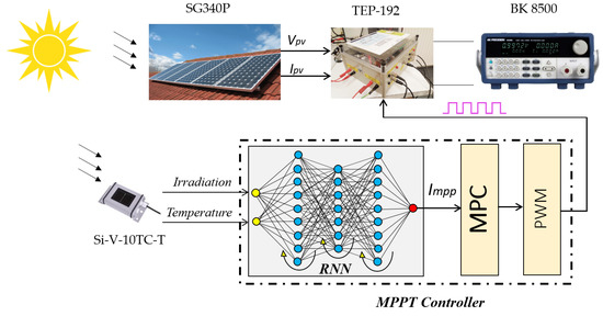
Figure 9.
Implementation architecture of the MPPT controller.
Table 2.
Technical data of PEIMAR SG340P.
Table 3.
TEP-192 Details.
Table 4.
BK 8500B Specifications.
3.2. Recurrent Neural Network
A RNN is a class of artificial neural networks that uses information from the previous iteration to ameliorate the performance of the NN in current and future inputs. In comparison with other networks, it can be said that RNN is unique because is the only network that contains a hidden state (memory) and loops. This structure allows the RNN to store past information in the hidden state and operate on sequences. In other words, it gets part of its output as an input for the next time step. These features are well suited for solving different problems with sequential data of varying length. Different RNN architectures, such as fully recurrent (FRNN), long short-term memory (LSTM), gated recurrent units (GRUs), etc., were introduced in recent decades. Due to its simplicity, the RNN configuration were used in many filtering and modeling applications. The hidden layer and the output of the RNN can be calculated using Equation (17).
where , , , are, respectively, the input vector, the hidden layer vector, and the output vector; W, U, and b, are parameter matrices and vector; and are activation functions, respectively, given in Equations (19) and (20).
To train the RNN model, we selected the temperature and irradiation as two input feature vectors while the output is the reference current vector that corresponds to the ongoing of the MPP. The dataset used in this work contains 796 normalized samples where 70% was used for the training, 15% for the validation and 15% for the test. Different training algorithms were checked so as to obtain an accurate model. Finally, we set the configuration of the LRN with the following parameters: training algorithm = Levenberg-Marquardt (LM), learning rate = 0.1, hidden layers = 2, neurons = 41, maximum epochs = 5000. The training performance was measured using mean square error (MSE, defined in Equation (21)), where the error is the difference between the predicted output and the target, and N is the number of training data. The predicted output, the target and the error are presented in Figure 10.
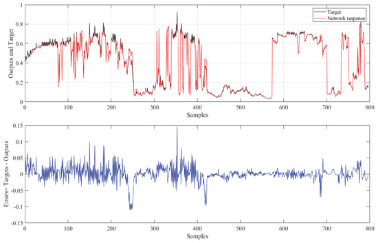
Figure 10.
Predicted outputs results.
The performance of the trained model can be analyzed using the regression values presented in Figure 11; where R represents the output-target relationship, which is ranged between 0 and 1 (0: low accuracy, 1: ideal accuracy). According to Figure 11, it is clear that the obtained RNN model is characterised by high prediction accuracy since the R values for training, validation and test are, respectively, equal to 0.99566, 0.99521 and 0.9936.
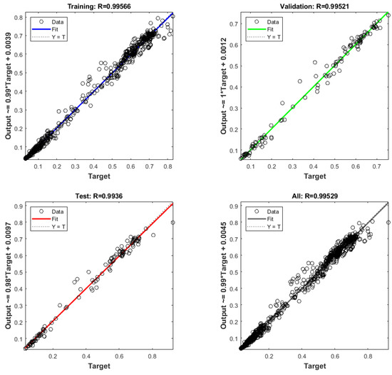
Figure 11.
Performance analysis of the predicted LRN model.
The characteristics of the current corresponds to the MPP for each temperature and irradiation, which are plotted in Figure 12. According to this figure, it is noticeable that the highest currents (yellow area) are found at high irradiation and low temperature, a reduction in the current can be occurred via an increase in temperature or via a decrease in irradiation. Moreover, the results from this figure show that the current is hardly affected by the irradiation in comparison with the temperature. Hence, for a constant irradiation and by increasing the temperature from 0 C to 50 C, the current of the maximum power is decreased around 2 A. On the other hand, for a constant temperature and by decreasing the irradiation from 900 W/m2 to 100 W/m2, the current of the maximum power is decreased around 7 A.
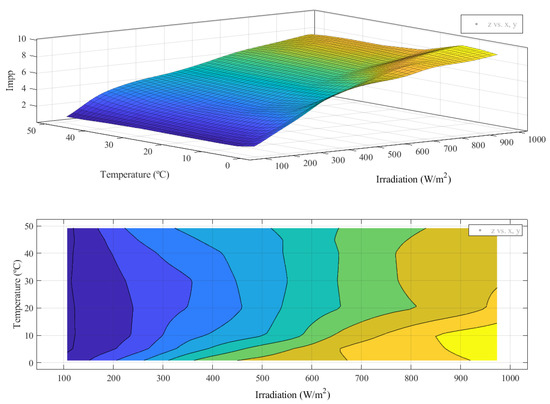
Figure 12.
characteristic surface of the MPP.
4. Results
4.1. PV Characteristics
The characteristic curves of the SG340P panel are shown in Figure 13; where the voltage-current features are presented in (a) and the voltage-power characteristics are displayed in (b). These curves were obtained by feeding the duty cycle signal of the boost converter with a triangular signal while maintaining the output resistance load constant. This is a consequence of varying the input voltage of the boost converter which implies to alter the PV voltage. The characteristics were recorded in an environment of temperature and irradiation between 10.5 C and 37.8 C and from 193 W/m2 to 808 W/m2, respectively.
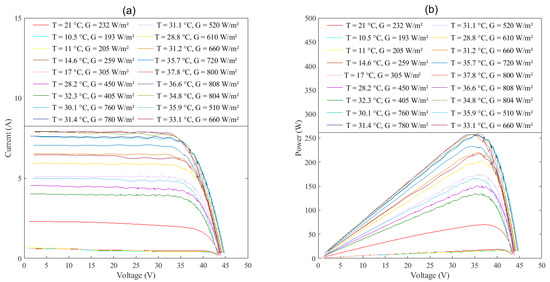
Figure 13.
PV panel characteristic curves: (a) voltage-current; (b) voltage–power.
4.2. P&O Results
The results of the P&O tracking method applied for the SG340P panel are presented in Figure 14 and Figure 15, where the irradiation, temperature, load resistance, duty cycle and current signal are, respectively, displayed from (a) to (e) in Figure 14; while the PV voltage signal, PV power, boost converter current, voltage and power, are, respectively, unveiled from (a) to (e) in Figure 15. A resistance load change was configured with a period of 120 s Figure 14c shows. The amplitude was configured in a square change from 30 to 35 that stayed constant for a certain time. Later, during the decrease, the change was from 35 to 30 . The schedule was configured with the aim of testing the algorithm performance at unexpected and complex disturbances. Several other unexpected effects such as sudden variation of the sun irradiation, which is resulting from the transitory cloud, are presented in Figure 14 as well. This variation directly affects the PV performance as can be seen at s of Figure 14e and Figure 15b,d,e.
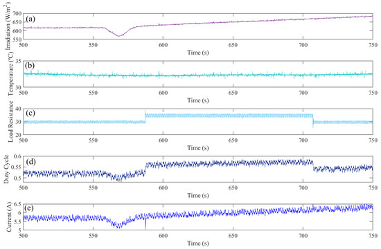
Figure 14.
MPPT based on P&O: (a) Irradiation (W/m2); (b) Temperature (C); (c) Load resistance (); (d) Duty cycle; (e) PV current.
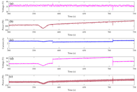
Figure 15.
MPPT based on P&O: (a) PV voltage; (b) PV power; (c) Boost converter output current; (d) Boost converter output voltage; (e) Boost converter output power.
Figure 14 and Figure 15 also reveal the behaviour of the P&O when facing unexpected load variation. Hence, it is clearly that the controller shows robustness for both load variations. However, chattering phenomenon with an amplitude of 0.3 A is also noticed in Figure 14e. This implies that some amount of the extracted power will be lost. Regarding to the performance of the boost converter, it is noticed that the output power (shown in Figure 15e) was reduced in comparison with the PV extracted power (displayed in Figure 15b). Actually, this is a usual behaviour since the converter was designed to deliver higher power, which implies that it will not be efficient at low power operation.
4.3. SMC Results
The results of the MPPT tracking method based on a combination of SMC and RNN are presented in Figure 16, Figure 17 and Figure 18. Certainly, the irradiation and temperature are different to the previous weather condition since the experiment was performed in diverse surroundings. The load resistance variation values which exhibited in Figure 17a were set the same as the previous P&O experiment. One advantage of the SMC is its implementation simplicity since it does not need high human skills.
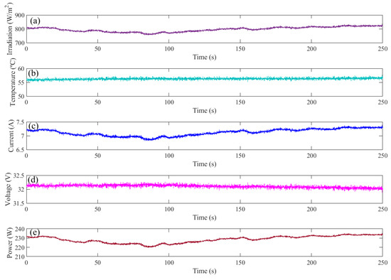
Figure 16.
MPPT based on RNN and SMC: (a) Irradiation (W/m2); (b) Temperature (C); (c) PV current; (d) PV voltage; (e) PV power.
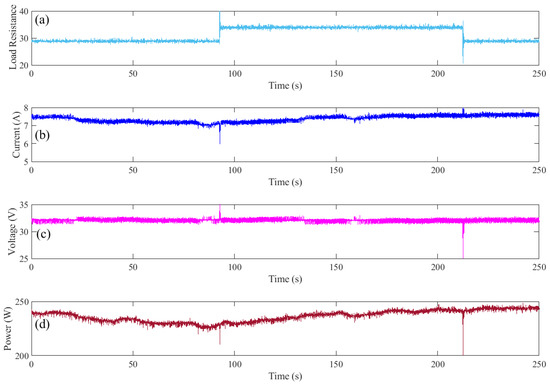
Figure 17.
MPPT based on RNN and SMC: (a) Load Resistance (); (b) PV current; (c) PV voltage; (d) PV power.
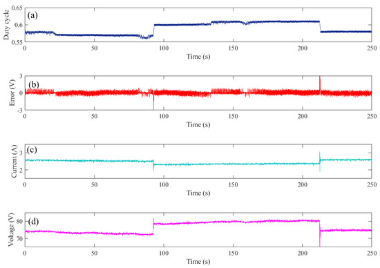
Figure 18.
MPPT based on RNN and SMC: (a) Duty cycle; (b) Error; (c) Boost converter output current (); (d) Boost converter output voltage ().
With regards to the PV controlled outputs, which are presented in Figure 17b–d, the first feature that can be highlighted over the P&O algorithm is the chattering reduction. This is clearly visible in Figure 17c where the amplitude is almost 1 V and it is almost 2 V with the case of the P&O algorithm. This phenomenon cutback is also clearly presented in the duty cycle signal which is depicted in Figure 18a, where the reduction is up to 70% in comparison with the duty cycle signal of the P&O which presented in Figure 14d. In reality, the SMC shows less chattering than the presented amplitudes because part of these amplitudes came from the chattering in the reference (Figure 16c,d) that generated by the RNN model. Another feature that should be highlighted is the robustness of the SMC. This latter faces the sharp load variations with high robustness since it forces the controlled signal to converge to the desired values with less than 1 s. Finally, it is important to mention that the SMC designed in this work is an error-based controller whereas the P&O is perturbation-based. The acquired error values of the SMC algorithm are displayed in Figure 18b, where the chattering amplitude of this scheme still its main drawback.
4.4. FLC Results
The results of the implementation of FLC and RNN for MPPT are presented in Figure 19, Figure 20 and Figure 21. The atmospheric conditions (irradiation and temperature) that supplied the RNN model are reflected in Figure 19a,b. The predicted MPP current , MPPT voltage and the maximum power are, respectively, displayed in Figure 19c–e.
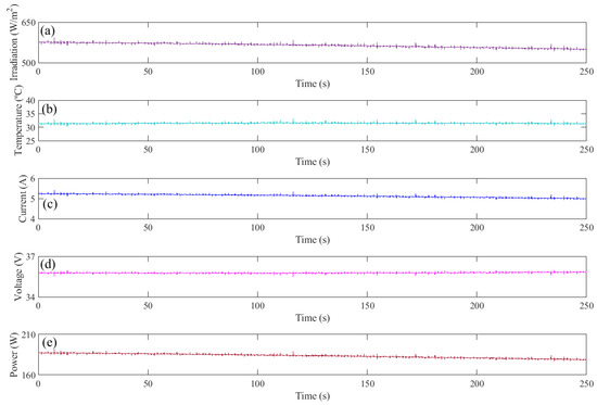
Figure 19.
MPPT based on RNN and FLC: (a) Irradiation (W/m2); (b) Temperature (C); (c) PV current; (d) PV voltage; (e) PV power.
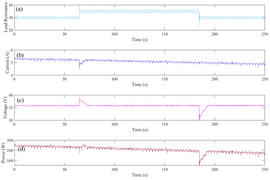
Figure 20.
MPPT based on RNN and FLC: (a) Load Resistance (); (b) PV current; (c) PV voltage; (d) PV power.
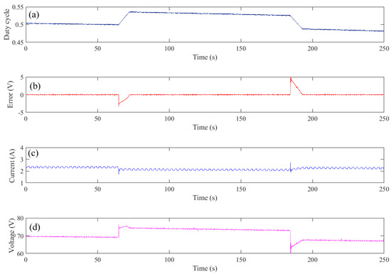
Figure 21.
MPPT based on RNN and FLC: (a) Duty cycle; (b) Error; (c) Boost converter output current (); (d) Boost converter output voltage ().
The performance of the FLC for tracking the , generated by the RNN model, is exhibited in Figure 20 and Figure 21. Initially, in comparison with the previous MPP tracking controllers, FLC performs better in terms of chattering reduction since the current ripple amplitude is less than 0.1 A as displayed in Figure 20b. This is also clearly presented in the voltage signal of Figure 20c which is almost vanished in comparison with the chattering voltage of the previous controllers. The ripples that appears in the load resistance of Figure 20a are consequence of an electrical relation of the output current and voltage (Figure 21c,d) since the programmable resistance lacks direct measurement. One disadvantage of the FLC found in the experiments when compared to the previous tracking controllers was its lack of robustness when facing sharp load variations. Hence, for both increasing and decreasing the load resistance, it takes around 10 s to reach the desired tracking value.
4.5. MPC Results
The results of the MPC tracking method are presented in Figure 22, Figure 23 and Figure 24. Figure 22 exhibits the irradiation, temperature, predicted current, voltage and power that corresponding to the MPP, while the performance of the MPC for tracking the are exhibited in Figure 23 and Figure 24. Despite that the experiments with the MPC were conducted under wide variation of irradiation, Figure 22 proves the effectiveness of the RNN model to track . Hence, it is clearly presented in Figure 22c that the predicted current fluctuates in the same way as the irradiation signal (displayed in Figure 22a). Moreover, the characteristic of the predicted power shown in Figure 22d is equivalent with the characteristic of the MPP previously shown in Figure 13. For instance, at s, the values extracted from Figure 22 for irradiation, temperature, current, voltage and power, are almost equal to the MPP characteristic values of the orange curve of Figure 13.
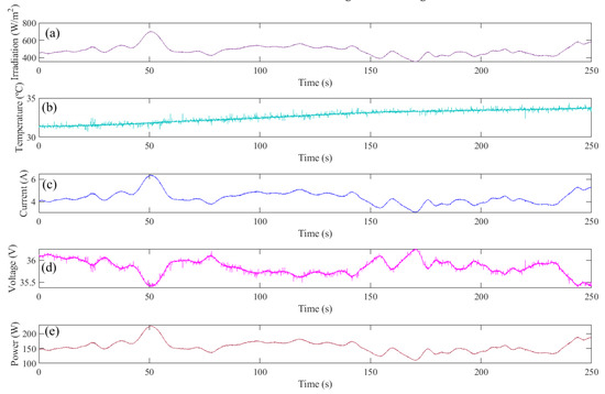
Figure 22.
MPPT based on RNN and MPC: (a) Irradiation (W/m2); (b) Temperature (C); (c) PV current; (d) PV voltage; (e) PV power.
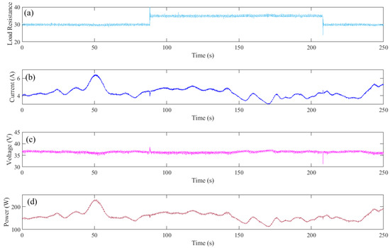
Figure 23.
MPPT based on RNN and MPC: (a) Load Resistance (); (b) PV current; (c) PV voltage; (d) PV power.
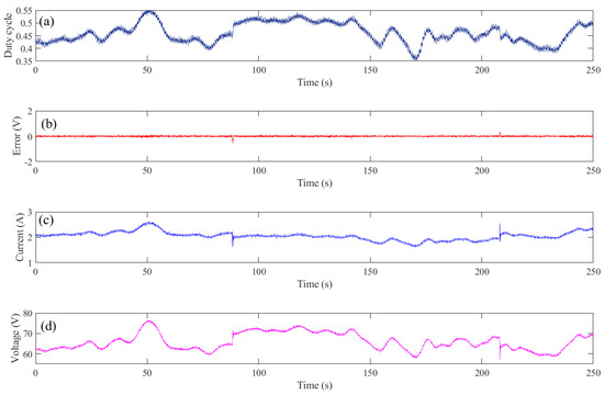
Figure 24.
MPPT based on RNN and MPC: (a) Duty cycle; (b) Error; (c) Boost converter output current (); (d) Boost converter output voltage ().
Regarding the demeanor of the MPC, it shows slight chattering reduction in contrast with P&O and SMC, while performing with high robustness in comparison with FLC. Hence, it takes only around 1 s as a response time when facing unexpected load variation. The performance of the MPC may not be so clear due to the high fluctuations of the irradiation which implies large variations in the PV outputs. However, the robustness and the high accuracy are clearly proven via the generated error signal which reflected in Figure 24b.
4.6. Comparison Results
To obtain high control performance, different metrics including integral of the absolute error, root-mean-square-error, relative root-mean-square-error and efficiency, were used in the experiments where the error signal should be reduced to improve the tracking accuracy. As a result, these metrics were minimized by tuning the corresponding gains for each controller, and therefore, the metrics in terms of error were determined during a period of two load variations. The obtained values for each metric are listed in Table 5.
Table 5.
Comparison of the different metrics.
According to these results, the IAE revealed an expected improvement for the MPC algorithm where the SMC and P&O showed values of 2.28 and 2.58 times higher than the FLC and values of 9.63 and 10.93 times higher than the MPC. For the RMSE and RRMSE metrics, the reflection has the similar trend for the same period. The MPC provides an RMSE and RRMSE of 0.0407 and 0.9088, whereas the FLC, SMC and P&O downgraded the performance of the RMSE to 0.1468, 0.2985 and 0.3369, and the performance of the RRMSE were downgraded to 3.0169, 4.0103 and 5.8871, respectively. Finally, the efficiency percentages of the tracking performance between the desired and actual maximum power showed that the MPC provides efficient results with 0.78% better than the FLC, 2.15% better than the SMC, and 2.27% better than the P&O.
5. Discussion
This review article presented an analysis of several types of MPPT methods for PV systems linked to a DC-DC boost converter. This is an important and cutting-edge topic since it allows to provide the maximum performance of energy conversion in solar cells, which are widely used as an efficient renewable energy.
In the first part, it was seen that there are two main categories of MPPT, mechanical and electrical. An initial option are mechanical ones which are far better for industrial environments, although the initial investment is high. Nevertheless, in alternative situations, the MPPT can also be achieved through a control law that can be designed for a DC-DC boost converter that provides a PWM signal. In this sense, four categories were analyzed based on previous studies. Offline techniques such as FOCV and FSCC are the most simple to implement since these are based on linear approximations. Nevertheless, PV systems tend to have nonlinear behaviour because of the weather conditions (like temperature, irradiation and shadowing) that vary along each day.
A further step was analyzed in the HC algorithms (P&O, INC and INR) which principle is to locate the MPP by means of the power-voltage slope sign. Despite that the implementation and computational requirements are simple and low, the major disadvantage resides on the problems due to partial shadowing. The latter effect produces local MPP and the algorithms tend to fall in this place rather than in a global one. Furthermore, other issues are related to sudden changes in the load in advanced algorithms like Drift-Free, which is its weak-point.
Intelligent techniques can be capable of dealing with previously mentioned downsides of HC algorithms. PSO is a stochastic process that is capable of dealing with complex problems through a simple optimization and fast convergence. A problem found in the literature review of this method is the risk of falling in a local MPP. A similar approach studied was GA, which is based on biological principles of evolution; this frameworks is capable of avoiding the local maximum issue. Nevertheless, because PSO and GA are optimization methods, they require high computational resources in the case of implementation in hardware. Another intelligent technique analyzed was FLC, of which the principle is rather based on the designer’s experience, which provides a tuning from the knowledge of the system. Nevertheless, the deficiency of this technique arises whenever the membership functions need to be increase and this induces a high load in the computational resources.
Other common control techniques were reviewed, such as SMC and MPC. Despite the chattering issue which generates energy consumption and reduces the lifespan of actuators, it was found that SMC is a robust strategy when system uncertainties are present. The last analyzed approach was MPC, which a model-based controller that is capable of generating a control action from an optimization gathered from future predictions and constraints. Major disadvantages of the latter are related on the numerical capabilities of a hardware to compute the optimization.
After the revision of several algorithms for MPPT, four of them were chosen to be implemented in an experimental PV platform with commercial hardware. Since the weather conditions varied for every experimental test, the analysis of each was performed individually without a graph overlapping. The tests were also carried with variable load to check each controller capabilities. P&O was the first to be implemented as one of the most used ones in industry; its efficiency for robustness at load variations was demonstrated, but it also showed chattering and had difficulties to deliver low-power. The second implementation was carried with SMC which was easy to embedded and out-came with enough robustness, although the chattering was significant. The third try was with FLC, which was capable of showing a reduction of power consumption as a consequence of chattering decline. Nevertheless, the disadvantages appeared with the robustness deficiency at the disturbance change due to the variable load. The last tested controller was MPC which was known by the authors due to previous experience. In this sense, the results showed outstanding performance in resemblance to the former structures. With a simple configuration that could avoid the computational saturation of the hardware, the outcomes displayed high accuracy and robustness.
For future perspectives as guidelines, the authors expect to test different designs in order to enhance the obtained structures. A testing of the hardware capabilities in terms of the MPC can be performed, although this can induce delays and damage risks in the equipment. Linked to previous suggestion, the implementation of optimization algorithm such as PSO or GA can be performed but with certain limitations in computational resources. Additional tests such as Hammerstein-Wiener nonlinear system identification tools or nonlinear auto-regressive exogenous models can be used as alternatives to ANNs.
6. Conclusions
In this review article, different methods of MPPT were revised. Theoretical and experimental perspectives were established and contrasted based on assets and drawbacks. These were analyzed based on computational requirements and easiness of implementation, according to previous carried out research. From this perspective, we conclude that:
- Mechanical MPPTs as sun-trackers have a high cost, which makes these strategies suitable for industrial environments rather than domestic.
- Offline-based algorithms are decent when low computational resources are available, although it is a linear approach.
- Hill-climbing methods are the most used ones in real application, despite that shadow and drifting are main concerns to tackle.
- Intelligent techniques are very sensitive consume high computational resources, despite that they can be able to reject issues such as local MPP falling or drifting.
- The SMC algorithm is a mainly robust approach which can provide suitable results but at the cost of high chattering risk. MPC is a reliable strategy as it is capable of predicting the future state but its sensitivity resides on the time parameters which could affect the hardware limitations.
- Under the weather conditions available during experiments and available hardware, it was shown that MPC under a simple settle, it can provide the best results in comparison with P&O, FLC, and SMC.
Author Contributions
Conceptualization, M.D., C.N. and O.B.; methodology, M.D. and C.N.; software, M.D. and C.N.; validation, M.D.; formal analysis, M.D. and P.F.-B.; investigation, M.D., C.N. and O.B.; resources, O.B. and J.S.; writing—original draft preparation, M.D. and C.N.; writing—review and editing, M.D., C.N., J.S., I.C. and O.B.; supervision, O.B.; project administration, O.B. All authors have read and agreed to the published version of the manuscript.
Funding
This research was funded by the Basque Government through the project EKOHEGAZ (ELKARTEK KK-2021/00092), by the Diputación Foral de Álava (DFA), through the project CONAVANTER, and by the UPV/EHU, through the project GIU20/063.
Institutional Review Board Statement
Not applicable.
Informed Consent Statement
Not applicable.
Data Availability Statement
Not applicable.
Acknowledgments
The authors wish to express their gratitude to the Basque Government, through the project EKOHEGAZ (ELKARTEK KK-2021/00092), to the Diputación Foral de Álava (DFA), through the project CONAVANTER, and to the UPV/EHU, through the project GIU20/063, for supporting this work.
Conflicts of Interest
The authors declare no conflict of interest.
Abbreviations
The following abbreviations are used in this manuscript:
| MPPT | Maximum power point tracking |
| PV | Photovoltaic system |
| BC | Boost converter |
| Poly-Si | Polycristalline silicon |
| CdTe | Cadmium Telluride |
| CIGS | Copper indium |
| IBC | Interdigitated back contact |
| FOCV | Fractional open-circuit voltage |
| FSCC | Fractional short-circuit current |
| HC | Hill climbing |
| P&O | Perturbation and observation |
| INC | Incremental conductance |
| INC | Incremental resistance |
| DF | Drift-free |
| FLC | Fuzzy logic controller |
| PSO | Particle swarm optimization |
| GA | Genetic algorithm |
| SMC | Sliding mode control |
| MPC | Model predictive control |
| RNN | Recurrent neural network |
| FF | Feedforward |
| RB | Radial basis |
| LSTM | Long short term memory |
| GRU | Gate recurrent unit |
| ANFIS | Adaptive neuro-fuzzy inference system |
References
- International Panel on Climate Change. Climate Change 2021: The Physical Science Basis; Technical Report; International Panel on Climate Change: Geneva, Switzerland, 2021. [Google Scholar]
- International Energy Agency. Net Zero by 2050; Technical Report; International Energy Agency: Paris, France, 2021. [Google Scholar]
- Sheng, R.; Du, J.; Liu, S.; Wang, C.; Wang, Z.; Liu, X. Solar Photovoltaic Investment Changes across China Regions Using a Spatial Shift-Share Analysis. Energies 2021, 14, 6418. [Google Scholar] [CrossRef]
- Adefarati, T.; Bansal, R. Chapter 2—Energizing Renewable Energy Systems and Distribution Generation. In Pathways to a Smarter Power System; Taşcıkaraoğlu, A., Erdinç, O., Eds.; Academic Press: London, UK, 2019; pp. 29–65. [Google Scholar] [CrossRef]
- Kapsalis, V.; Kyriakopoulos, G.; Zamparas, M.; Tolis, A. Investigation of the Photon to Charge Conversion and Its Implication on Photovoltaic Cell Efficient Operation. Energies 2021, 14, 3022. [Google Scholar] [CrossRef]
- Dharmadasa, I.M.; Ojo, A.A.; Salim, H.I.; Dharmadasa, R. Next Generation Solar Cells Based on Graded Bandgap Device Structures Utilising Rod-Type Nano-Materials. Energies 2015, 8, 5440–5458. [Google Scholar] [CrossRef] [Green Version]
- Leitão, D.; Torres, J.P.N.; Fernandes, J.F.P. Spectral Irradiance Influence on Solar Cells Efficiency. Energies 2020, 13, 5017. [Google Scholar] [CrossRef]
- Romeo, A.; Artegiani, E. CdTe-Based Thin Film Solar Cells: Past, Present and Future. Energies 2021, 14, 1684. [Google Scholar] [CrossRef]
- Lee, S.; Bae, S.; Park, S.J.; Gwak, J.; Yun, J.; Kang, Y.; Kim, D.; Eo, Y.J.; Lee, H.S. Characterization of Potential-Induced Degradation and Recovery in CIGS Solar Cells. Energies 2021, 14, 4628. [Google Scholar] [CrossRef]
- Kumar, N.M.; Chopra, S.S.; Malvoni, M.; Elavarasan, R.M.; Das, N. Solar Cell Technology Selection for a PV Leaf Based on Energy and Sustainability Indicators—A Case of a Multilayered Solar Photovoltaic Tree. Energies 2020, 13, 6439. [Google Scholar] [CrossRef]
- Franklin, E.; Fong, K.; McIntosh, K.; Fell, A.; Blakers, A.; Kho, T.; Walter, D.; Wang, D.; Zin, N.; Stocks, M.; et al. Design, fabrication and characterisation of a 24.4% efficient interdigitated back contact solar cell. Prog. Photovolt. Res. Appl. 2016, 24, 411–427. [Google Scholar] [CrossRef]
- Li, X.; Liu, A. Carrier Transmission Mechanism-Based Analysis of Front Surface Field Effects on Simplified Industrially Feasible Interdigitated Back Contact Solar Cells. Energies 2020, 13, 5303. [Google Scholar] [CrossRef]
- Lin, B.R. Implementation of a Resonant Converter with Topology Morphing to Achieve Bidirectional Power Flow. Energies 2021, 14, 5186. [Google Scholar] [CrossRef]
- Bansal, S.; Saini, L.M.; Joshi, D. Design of a DC-DC converter for photovoltaic solar system. In Proceedings of the 2012 IEEE 5th India International Conference on Power Electronics (IICPE), Delhi, India, 6–8 December 2012; pp. 1–5. [Google Scholar] [CrossRef]
- Raghavendra, K.V.G.; Zeb, K.; Muthusamy, A.; Krishna, T.N.V.; Kumar, S.V.S.; Kim, D.H.; Kim, M.S.; Cho, H.G.; Kim, H.J. A Comprehensive Review of DC–DC Converter Topologies and Modulation Strategies with Recent Advances in Solar Photovoltaic Systems. Electronics 2020, 9, 31. [Google Scholar] [CrossRef] [Green Version]
- Kumar, R.; Wu, C.C.; Liu, C.Y.; Hsiao, Y.L.; Chieng, W.H.; Chang, E.Y. Discontinuous Current Mode Modeling and Zero Current Switching of Flyback Converter. Energies 2021, 14, 5996. [Google Scholar] [CrossRef]
- Farzan Moghaddam, A.; Van den Bossche, A. Forward Converter Current Fed Equalizer for Lithium Based Batteries in Ultralight Electrical Vehicles. Electronics 2019, 8, 408. [Google Scholar] [CrossRef] [Green Version]
- Hinov, N. Quasi-Boundary Method for Design Consideration of Resonant DC-DC Converters. Energies 2021, 14, 6153. [Google Scholar] [CrossRef]
- Duan, Q.; Li, Y.; Dai, X.; Zou, T. A Novel High Controllable Voltage Gain Push-Pull Topology for Wireless Power Transfer System. Energies 2017, 10, 474. [Google Scholar] [CrossRef] [Green Version]
- Tseng, S.Y.; Fan, J.H. Soft-Switching Full-Bridge Converter with Multiple-Input Sources for DC Distribution Applications. Symmetry 2021, 13, 775. [Google Scholar] [CrossRef]
- Mumtaz, F.; Zaihar Yahaya, N.; Tanzim Meraj, S.; Singh, B.; Kannan, R.; Ibrahim, O. Review on non-isolated DC-DC converters and their control techniques for renewable energy applications. Ain Shams Eng. J. 2021, 12, 3747–3763. [Google Scholar] [CrossRef]
- Farzan Moghaddam, A.; Van den Bossche, A. A Cuk Converter Cell Balancing Technique by Using Coupled Inductors for Lithium-Based Batteries. Energies 2019, 12, 2881. [Google Scholar] [CrossRef] [Green Version]
- Premkumar, M.; Subramaniam, U.; Haes Alhelou, H.; Siano, P. Design and Development of Non-Isolated Modified SEPIC DC-DC Converter Topology for High-Step-Up Applications: Investigation and Hardware Implementation. Energies 2020, 13, 3960. [Google Scholar] [CrossRef]
- Derbeli, M.; Barambones, O.; Ramos-Hernanz, J.A.; Sbita, L. Real-Time Implementation of a Super Twisting Algorithm for PEM Fuel Cell Power System. Energies 2019, 12, 1594. [Google Scholar] [CrossRef] [Green Version]
- Dimitrov, B.; Hayatleh, K.; Barker, S.; Collier, G.; Sharkh, S.; Cruden, A. A Buck-Boost Transformerless DC–DC Converter Based on IGBT Modules for Fast Charge of Electric Vehicles. Electronics 2020, 9, 397. [Google Scholar] [CrossRef] [Green Version]
- Kamaraj, V.; Chellammal, N.; Chokkalingam, B.; Munda, J.L. Minimization of Cross-Regulation in PV and Battery Connected Multi-Input Multi-Output DC to DC Converter. Energies 2020, 13, 6534. [Google Scholar] [CrossRef]
- Luo, F.L.; Ye, H. Ultra-lift Luo-converter. In Proceedings of the 2004 International Conference on Power System Technology (PowerCon 2004), Singapore, 21–24 November 2004; Volume 1, pp. 81–86. [Google Scholar] [CrossRef]
- Gursoy, M.; Zhuo, G.; Lozowski, A.G.; Wang, X. Photovoltaic Energy Conversion Systems with Sliding Mode Control. Energies 2021, 14, 6071. [Google Scholar] [CrossRef]
- Rasheduzzaman, M.; Fajri, P.; Kimball, J.; Deken, B. Modeling, Analysis, and Control Design of a Single-Stage Boost Inverter. Energies 2021, 14, 4098. [Google Scholar] [CrossRef]
- Javed, M.Y.; Mirza, A.F.; Hasan, A.; Rizvi, S.T.H.; Ling, Q.; Gulzar, M.M.; Safder, M.U.; Mansoor, M. A Comprehensive Review on a PV Based System to Harvest Maximum Power. Electronics 2019, 8, 1480. [Google Scholar] [CrossRef] [Green Version]
- Ali, A.; Irshad, K.; Khan, M.F.; Hossain, M.M.; Al-Duais, I.N.A.; Malik, M.Z. Artificial Intelligence and Bio-Inspired Soft Computing-Based Maximum Power Plant Tracking for a Solar Photovoltaic System under Non-Uniform Solar Irradiance Shading Conditions—A Review. Sustainability 2021, 13, 10575. [Google Scholar] [CrossRef]
- Ali, A.; Almutairi, K.; Malik, M.Z.; Irshad, K.; Tirth, V.; Algarni, S.; Zahir, M.H.; Islam, S.; Shafiullah, M.; Shukla, N.K. Review of Online and Soft Computing Maximum Power Point Tracking Techniques under Non-Uniform Solar Irradiation Conditions. Energies 2020, 13, 3256. [Google Scholar] [CrossRef]
- Al-Quraan, A.; Al-Qaisi, M. Modelling, Design and Control of a Standalone Hybrid PV-Wind Micro-Grid System. Energies 2021, 14, 4849. [Google Scholar] [CrossRef]
- Jager-Waldau, A. Snapshot of Photovoltaics—February 2020. Energies 2020, 13, 930. [Google Scholar] [CrossRef] [Green Version]
- Szindler, M.; Szindler, M.; Drygała, A.; Lukaszkowicz, K.; Kaim, P.; Pietruszka, R. Dye-Sensitized Solar Cell for Building-Integrated Photovoltaic (BIPV) Applications. Materials 2021, 14, 3743. [Google Scholar] [CrossRef]
- Abdel-Salam, M.; EL-Mohandes, M.T. History of Maximum Power Point Tracking. In Modern Maximum Power Point Tracking Techniques for Photovoltaic Energy Systems; Springer: Cham, Switzerland, 2019; pp. 1–29. [Google Scholar] [CrossRef]
- Murtaza, A.; Chiaberge, M.; De Giuseppe, M.; Boero, D. A duty cycle optimization based hybrid maximum power point tracking technique for photovoltaic systems. Int. J. Electr. Power Energy Syst. 2014, 59, 141–154. [Google Scholar] [CrossRef]
- Murtaza, A.; Chiaberge, M.; Spertino, F.; Boero, D.; De Giuseppe, M. A maximum power point tracking technique based on bypass diode mechanism for PV arrays under partial shading. Energy Build. 2014, 73, 13–25. [Google Scholar] [CrossRef]
- Islam, H.; Mekhilef, S.; Shah, N.B.M.; Soon, T.K.; Seyedmahmousian, M.; Horan, B.; Stojcevski, A. Performance Evaluation of Maximum Power Point Tracking Approaches and Photovoltaic Systems. Energies 2018, 11, 365. [Google Scholar] [CrossRef] [Green Version]
- Awasthi, A.; Shukla, A.K.; Murali Manohar, S.R.; Dondariya, C.; Shukla, K.N.; Porwal, D.; Richhariya, G. Review on sun tracking technology in solar PV system. Energy Rep. 2020, 6, 392–405. [Google Scholar] [CrossRef]
- Albalawi, H.; Zaid, S.A. An H5 Transformerless Inverter for Grid Connected PV Systems with Improved Utilization Factor and a Simple Maximum Power Point Algorithm. Energies 2018, 11, 2912. [Google Scholar] [CrossRef] [Green Version]
- Windarko, N.A.; Nizar Habibi, M.; Sumantri, B.; Prasetyono, E.; Efendi, M.Z.; Taufik. A New MPPT Algorithm for Photovoltaic Power Generation under Uniform and Partial Shading Conditions. Energies 2021, 14, 483. [Google Scholar] [CrossRef]
- Gosumbonggot, J.; Fujita, G. Partial Shading Detection and Global Maximum Power Point Tracking Algorithm for Photovoltaic with the Variation of Irradiation and Temperature. Energies 2019, 12, 202. [Google Scholar] [CrossRef] [Green Version]
- Tchoketch Kebir, G.F.; Larbes, C.; Ilinca, A.; Obeidi, T.; Tchoketch Kebir, S. Study of the Intelligent Behavior of a Maximum Photovoltaic Energy Tracking Fuzzy Controller. Energies 2018, 11, 3263. [Google Scholar] [CrossRef] [Green Version]
- Baimel, D.; Tapuchi, S.; Levron, Y.; Belikov, J. Improved Fractional Open Circuit Voltage MPPT Methods for PV Systems. Electronics 2019, 8, 321. [Google Scholar] [CrossRef] [Green Version]
- Owusu-Nyarko, I.; Elgenedy, M.A.; Abdelsalam, I.; Ahmed, K.H. Modified Variable Step-Size Incremental Conductance MPPT Technique for Photovoltaic Systems. Electronics 2021, 10, 2331. [Google Scholar] [CrossRef]
- Nivedha, S.; Vijayalaxmi, M. Performance Analysis of Fuzzy based Hybrid MPPT Algorithm for Photovoltaic system. In Proceedings of the 2021 International Conference on Communication, Control and Information Sciences (ICCISc), Virtual, 16–18 June 2021; Volume 1, pp. 1–4. [Google Scholar] [CrossRef]
- Mohamed Hariri, M.H.; Mat Desa, M.K.; Masri, S.; Mohd Zainuri, M.A.A. Grid-Connected PV Generation System—Components and Challenges: A Review. Energies 2020, 13, 4279. [Google Scholar] [CrossRef]
- Frezzetti, A.; Manfredi, S.; Suardi, A. Adaptive FOCV-based Control Scheme to improve the MPP Tracking Performance: An experimental validation. IFAC Proc. Vol. 2014, 47, 4967–4971. [Google Scholar] [CrossRef] [Green Version]
- Sher, H.A.; Murtaza, A.F.; Noman, A.; Addoweesh, K.E.; Al-Haddad, K.; Chiaberge, M. A New Sensorless Hybrid MPPT Algorithm Based on Fractional Short-Circuit Current Measurement and P&O MPPT. IEEE Trans. Sustain. Energy 2015, 6, 1426–1434. [Google Scholar] [CrossRef] [Green Version]
- Lee, H.S.; Yun, J.J. Advanced MPPT Algorithm for Distributed Photovoltaic Systems. Energies 2019, 12, 3576. [Google Scholar] [CrossRef] [Green Version]
- Yildirim, M.A.; Nowak-Ocłoń, M. Modified Maximum Power Point Tracking Algorithm under Time-Varying Solar Irradiation. Energies 2020, 13, 6722. [Google Scholar] [CrossRef]
- Murtaza, A.F.; Sher, H.A.; Spertino, F.; Ciocia, A.; Noman, A.M.; Al-Shamma’a, A.A.; Alkuhayli, A. A Novel MPPT Technique Based on Mutual Coordination between Two PV Modules/Arrays. Energies 2021, 14, 6996. [Google Scholar] [CrossRef]
- Louzazni, M.; Cotfas, D.T.; Cotfas, P.A. Management and Performance Control Analysis of Hybrid Photovoltaic Energy Storage System under Variable Solar Irradiation. Energies 2020, 13, 3043. [Google Scholar] [CrossRef]
- Aourir, J.; Locment, F. Limited Power Point Tracking for a Small-Scale Wind Turbine Intended to Be Integrated in a DC Microgrid. Appl. Sci. 2020, 10, 8030. [Google Scholar] [CrossRef]
- Mahmod Mohammad, A.N.; Mohd Radzi, M.A.; Azis, N.; Shafie, S.; Atiqi Mohd Zainuri, M.A. An Enhanced Adaptive Perturb and Observe Technique for Efficient Maximum Power Point Tracking Under Partial Shading Conditions. Appl. Sci. 2020, 10, 3912. [Google Scholar] [CrossRef]
- Gil-Antonio, L.; Saldivar, B.; Portillo-Rodríguez, O.; Ávila Vilchis, J.C.; Martínez-Rodríguez, P.R.; Martínez-Méndez, R. Flatness-Based Control for the Maximum Power Point Tracking in a Photovoltaic System. Energies 2019, 12, 1843. [Google Scholar] [CrossRef] [Green Version]
- Veerachary, M. Fourth-order buck converter for maximum power point tracking applications. IEEE Trans. Aerosp. Electron. Syst. 2011, 47, 896–911. [Google Scholar] [CrossRef]
- Singh, G.K. Solar power generation by PV (photovoltaic) technology: A review. Energy 2013, 53, 1–13. [Google Scholar] [CrossRef]
- Ishaque, K.; Salam, Z.; Lauss, G. The performance of perturb and observe and incremental conductance maximum power point tracking method under dynamic weather conditions. Appl. Energy 2014, 119, 228–236. [Google Scholar] [CrossRef]
- Li, C.; Chen, Y.; Zhou, D.; Liu, J.; Zeng, J. A High-Performance Adaptive Incremental Conductance MPPT Algorithm for Photovoltaic Systems. Energies 2016, 9, 288. [Google Scholar] [CrossRef] [Green Version]
- Mei, Q.; Shan, M.; Liu, L.; Guerrero, J.M. A Novel Improved Variable Step-Size Incremental-Resistance MPPT Method for PV Systems. IEEE Trans. Ind. Electron. 2011, 58, 2427–2434. [Google Scholar] [CrossRef]
- Jately, V.; Azzopardi, B.; Joshi, J.; Venkateswaran V, B.; Sharma, A.; Arora, S. Experimental Analysis of hill-climbing MPPT algorithms under low irradiance levels. Renew. Sustain. Energy Rev. 2021, 150, 111467. [Google Scholar] [CrossRef]
- Raedani, R.; Hanif, M. Design, testing and comparison of P&O, IC and VSSIR MPPT techniques. In Proceedings of the 2014 International Conference on Renewable Energy Research and Application (ICRERA), Milwaukee, WI, USA, 19–22 October 2014; pp. 322–330. [Google Scholar] [CrossRef]
- AHMED, E.; Shoyama, M. Scaling Factor Design Based Variable Step Size Incremental Resistance Maximum Power Point Tracking for PV Systems. J. Power Electron. 2012, 12, 164–171. [Google Scholar] [CrossRef]
- Killi, M.; Samanta, S. Modified Perturb and Observe MPPT Algorithm for Drift Avoidance in Photovoltaic Systems. IEEE Trans. Ind. Electron. 2015, 62, 5549–5559. [Google Scholar] [CrossRef]
- Mathew, J.; Beevi, S.S.; Vincent, G. Model based MPPT algorithm for drift-free operation in PV systems under rapidly varying climatic conditions. In Proceedings of the 2016 7th India International Conference on Power Electronics (IICPE), Patiala, India, 17–19 November 2016; pp. 1–5. [Google Scholar] [CrossRef]
- Kumar, V.; Singh, M. Derated Mode of Power Generation in PV System Using Modified Perturb and Observe MPPT Algorithm. J. Mod. Power Syst. Clean Energy 2021, 9, 1183–1192. [Google Scholar] [CrossRef]
- Larbes, C.; Aït Cheikh, S.; Obeidi, T.; Zerguerras, A. Genetic algorithms optimized fuzzy logic control for the maximum power point tracking in photovoltaic system. Renew. Energy 2009, 34, 2093–2100. [Google Scholar] [CrossRef]
- Robles Algarín, C.; Taborda Giraldo, J.; Rodríguez Álvarez, O. Fuzzy Logic Based MPPT Controller for a PV System. Energies 2017, 10, 2036. [Google Scholar] [CrossRef] [Green Version]
- Volosencu, C. Reducing Energy Consumption and Increasing the Performances of AC Motor Drives Using Fuzzy PI Speed Controllers. Energies 2021, 14, 2083. [Google Scholar] [CrossRef]
- Nicolosi, G.; Volpe, R.; Messineo, A. An Innovative Adaptive Control System to Regulate Microclimatic Conditions in a Greenhouse. Energies 2017, 10, 722. [Google Scholar] [CrossRef] [Green Version]
- Hussain, S.; Lee, K.B.; Ahmed, M.A.; Hayes, B.; Kim, Y.C. Two-Stage Fuzzy Logic Inference Algorithm for Maximizing the Quality of Performance under the Operational Constraints of Power Grid in Electric Vehicle Parking Lots. Energies 2020, 13, 4634. [Google Scholar] [CrossRef]
- Hinokuma, T.; Farzaneh, H.; Shaqour, A. Techno-Economic Analysis of a Fuzzy Logic Control Based Hybrid Renewable Energy System to Power a University Campus in Japan. Energies 2021, 14, 1960. [Google Scholar] [CrossRef]
- Al-Majidi, S.D.; Abbod, M.F.; Al-Raweshidy, H.S. A novel maximum power point tracking technique based on fuzzy logic for photovoltaic systems. Int. J. Hydrogen Energy 2018, 43, 14158–14171. [Google Scholar] [CrossRef]
- Bakkar, M.; Aboelhassan, A.; Abdelgeliel, M.; Galea, M. PV Systems Control Using Fuzzy Logic Controller Employing Dynamic Safety Margin under Normal and Partial Shading Conditions. Energies 2021, 14, 841. [Google Scholar] [CrossRef]
- Tahan, M.; Bamgboje, D.O.; Hu, T. Compensated Single Input Multiple Output Flyback Converter. Energies 2021, 14, 3009. [Google Scholar] [CrossRef]
- Camboim, M.M.; Villanueva, J.M.M.; de Souza, C.P. Fuzzy Controller Applied to a Remote Energy Harvesting Emulation Platform. Sensors 2020, 20, 5874. [Google Scholar] [CrossRef]
- Napole, C.; Derbeli, M.; Barambones, O. A global integral terminal sliding mode control based on a novel reaching law for a proton exchange membrane fuel cell system. Appl. Energy 2021, 301, 117473. [Google Scholar] [CrossRef]
- Al-Majidi, S.D.; Abbod, M.F.; Al-Raweshidy, H.S. Design of an Efficient Maximum Power Point Tracker Based on ANFIS Using an Experimental Photovoltaic System Data. Electronics 2019, 8, 858. [Google Scholar] [CrossRef] [Green Version]
- Salleh, M.N.M.; Talpur, N.; Hussain, K. Adaptive Neuro-Fuzzy Inference System: Overview, Strengths, Limitations, and Solutions. In Data Mining and Big Data; Springer International Publishing: Cham, Switzerland, 2017. [Google Scholar]
- Torres-Madroñero, J.L.; Nieto-Londoño, C.; Sierra-Pérez, J. Hybrid Energy Systems Sizing for the Colombian Context: A Genetic Algorithm and Particle Swarm Optimization Approach. Energies 2020, 13, 5648. [Google Scholar] [CrossRef]
- Mohamed, M.A.; Zaki Diab, A.A.; Rezk, H. Partial shading mitigation of PV systems via different meta-heuristic techniques. Renew. Energy 2019, 130, 1159–1175. [Google Scholar] [CrossRef]
- Shen, Y.; Cai, W.; Kang, H.; Sun, X.; Chen, Q.; Zhang, H. A Particle Swarm Algorithm Based on a Multi-Stage Search Strategy. Entropy 2021, 23, 1200. [Google Scholar] [CrossRef]
- Hayder, W.; Ogliari, E.; Dolara, A.; Abid, A.; Ben Hamed, M.; Sbita, L. Improved PSO: A Comparative Study in MPPT Algorithm for PV System Control under Partial Shading Conditions. Energies 2020, 13, 2035. [Google Scholar] [CrossRef]
- Alshareef, M.; Lin, Z.; Ma, M.; Cao, W. Accelerated Particle Swarm Optimization for Photovoltaic Maximum Power Point Tracking under Partial Shading Conditions. Energies 2019, 12, 623. [Google Scholar] [CrossRef] [Green Version]
- Shaari, G.; Tekbiyik-Ersoy, N.; Dagbasi, M. The State of Art in Particle Swarm Optimization Based Unit Commitment: A Review. Processes 2019, 7, 733. [Google Scholar] [CrossRef] [Green Version]
- Dehghani, M.; Hubalovsky, S.; Trojovsky, P. Cat and Mouse Based Optimizer: A New Nature-Inspired Optimization Algorithm. Sensors 2021, 21, 5214. [Google Scholar] [CrossRef]
- Lee, H.; Kim, K.; Kwon, Y.; Hong, E. Real-Time Particle Swarm Optimization on FPGA for the Optimal Message-Chain Structure. Electronics 2018, 7, 274. [Google Scholar] [CrossRef] [Green Version]
- Al-Majidi, S.D.; Abbod, M.F.; Al-Raweshidy, H.S. A particle swarm optimisation-trained feedforward neural network for predicting the maximum power point of a photovoltaic array. Eng. Appl. Artif. Intell. 2020, 92, 103688. [Google Scholar] [CrossRef]
- Dehghani, M.; Mardaneh, M.; Malik, O.P.; Guerrero, J.M.; Sotelo, C.; Sotelo, D.; Nazari-Heris, M.; Al-Haddad, K.; Ramirez-Mendoza, R.A. Genetic Algorithm for Energy Commitment in a Power System Supplied by Multiple Energy Carriers. Sustainability 2020, 12, 10053. [Google Scholar] [CrossRef]
- Daraban, S.; Petreus, D.; Morel, C. A novel MPPT (maximum power point tracking) algorithm based on a modified genetic algorithm specialized on tracking the global maximum power point in photovoltaic systems affected by partial shading. Energy 2014, 74, 374–388. [Google Scholar] [CrossRef]
- Zagrouba, M.; Sellami, A.; Bouaïcha, M.; Ksouri, M. Identification of PV solar cells and modules parameters using the genetic algorithms: Application to maximum power extraction. Sol. Energy 2010, 84, 860–866. [Google Scholar] [CrossRef]
- Mirnateghi, E.; Mosallam, A.S. Multi-Criteria Optimization of Energy-Efficient Cementitious Sandwich Panels Building Systems Using Genetic Algorithm. Energies 2021, 14, 6001. [Google Scholar] [CrossRef]
- Lee, J.; Jeong, S. Robust Temperature Control of a Variable-Speed Refrigeration System Based on Sliding Mode Control with Optimal Parameters Derived Using the Genetic Algorithm. Energies 2021, 14, 6321. [Google Scholar] [CrossRef]
- Hua, C.C.; Zhan, Y.J. A Hybrid Maximum Power Point Tracking Method without Oscillations in Steady-State for Photovoltaic Energy Systems. Energies 2021, 14, 5590. [Google Scholar] [CrossRef]
- Megantoro, P.; Nugroho, Y.D.; Anggara, F.; Suhono; Rusadi, E.Y. Simulation and Characterization of Genetic Algorithm Implemented on MPPT for PV System under Partial Shading Condition. In Proceedings of the 2018 3rd International Conference on Information Technology, Information System and Electrical Engineering (ICITISEE), Yogyakarta, Indonesia, 13–14 November 2018; pp. 74–78. [Google Scholar] [CrossRef]
- Chao, K.H.; Rizal, M.N. A Hybrid MPPT Controller Based on the Genetic Algorithm and Ant Colony Optimization for Photovoltaic Systems under Partially Shaded Conditions. Energies 2021, 14, 2902. [Google Scholar] [CrossRef]
- Attarmoghaddam, N.; Li, K.F.; Kanan, A. FPGA Implementation of Crossover Module of Genetic Algorithm. Information 2019, 10, 184. [Google Scholar] [CrossRef] [Green Version]
- Wang, Z.; Wang, Y.; Zhang, L.; Liu, M. Vehicle Stability Enhancement through Hierarchical Control for a Four-Wheel-Independently-Actuated Electric Vehicle. Energies 2017, 10, 947. [Google Scholar] [CrossRef] [Green Version]
- Derbeli, M.; Farhat, M.; Barambones, O.; Sbita, L. Control of PEM fuel cell power system using sliding mode and super-twisting algorithms. Int. J. Hydrogen Energy 2017, 42, 8833–8844. [Google Scholar] [CrossRef]
- Kali, Y.; Ayala, M.; Rodas, J.; Saad, M.; Doval-Gandoy, J.; Gregor, R.; Benjelloun, K. Current Control of a Six-Phase Induction Machine Drive Based on Discrete-Time Sliding Mode with Time Delay Estimation. Energies 2019, 12, 170. [Google Scholar] [CrossRef] [Green Version]
- Kihal, A.; Krim, F.; Talbi, B.; Laib, A.; Sahli, A. A Robust Control of Two-Stage Grid-Tied PV Systems Employing Integral Sliding Mode Theory. Energies 2018, 11, 2791. [Google Scholar] [CrossRef] [Green Version]
- Chouza, A.; Barambones, O.; Calvo, I.; Velasco, J. Sliding Mode-Based Robust Control for Piezoelectric Actuators with Inverse Dynamics Estimation. Energies 2019, 12, 943. [Google Scholar] [CrossRef] [Green Version]
- Silaa, M.Y.; Derbeli, M.; Barambones, O.; Cheknane, A. Design and implementation of high order sliding mode control for PEMFC power system. Energies 2020, 13, 4317. [Google Scholar] [CrossRef]
- Ramos-Paja, C.A.; Gonzalez Montoya, D.; Bastidas-Rodriguez, J.D. Sliding-Mode Control of Distributed Maximum Power Point Tracking Converters Featuring Overvoltage Protection. Energies 2018, 11, 2220. [Google Scholar] [CrossRef] [Green Version]
- Gao, Y.; Li, X.; Zhang, W.; Hou, D.; Zheng, L. A Sliding Mode Control Strategy with Repetitive Sliding Surface for Shunt Active Power Filter with an LCLCL Filter. Energies 2020, 13, 1740. [Google Scholar] [CrossRef] [Green Version]
- Pan, L.; Zhu, Z.; Xiong, Y.; Shao, J. Integral Sliding Mode Control for Maximum Power Point Tracking in DFIG Based Floating Offshore Wind Turbine and Power to Gas. Processes 2021, 9, 1016. [Google Scholar] [CrossRef]
- Garcia-Torres, F.; Zafra-Cabeza, A.; Silva, C.; Grieu, S.; Darure, T.; Estanqueiro, A. Model Predictive Control for Microgrid Functionalities: Review and Future Challenges. Energies 2021, 14, 1296. [Google Scholar] [CrossRef]
- Serale, G.; Fiorentini, M.; Capozzoli, A.; Bernardini, D.; Bemporad, A. Model Predictive Control (MPC) for Enhancing Building and HVAC System Energy Efficiency: Problem Formulation, Applications and Opportunities. Energies 2018, 11, 631. [Google Scholar] [CrossRef] [Green Version]
- Bououden, S.; Hazil, O.; Filali, S.; Chadli, M. Modelling and model predictive control of a DC-DC Boost converter. In Proceedings of the 2014 15th International Conference on Sciences and Techniques of Automatic Control and Computer Engineering (STA), Hammamet, Tunisia, 21–23 December 2014; pp. 643–648. [Google Scholar]
- Derbeli, M.; Charaabi, A.; Barambones, O.; Napole, C. High-Performance Tracking for Proton Exchange Membrane Fuel Cell System PEMFC Using Model Predictive Control. Mathematics 2021, 9, 1158. [Google Scholar] [CrossRef]
- Muñoz, C.; Rivera, M.; Villalón, A.; Baier, C.R.; Muñoz, J.; Ramirez, R.O.; Wheeler, P. Predictive Control with Current-Based Maximum Power Point-Tracking for On-Grid Photovoltaic Applications. Sustainability 2021, 13, 3037. [Google Scholar] [CrossRef]
- Oh, S.; Chae, S.; Neely, J.; Baek, J.; Cook, M. Efficient Model Predictive Control Strategies for Resource Management in an Islanded Microgrid. Energies 2017, 10, 1008. [Google Scholar] [CrossRef]
- Wang, F.; Zhang, Z.; Mei, X.; Rodríguez, J.; Kennel, R. Advanced Control Strategies of Induction Machine: Field Oriented Control, Direct Torque Control and Model Predictive Control. Energies 2018, 11, 120. [Google Scholar] [CrossRef] [Green Version]
- Choi, Y.; Lee, W.; Kim, J.; Yoo, J. A Variable-Sampling Time Model Predictive Control Algorithm for Improving Path-Tracking Performance of a Vehicle. Sensors 2021, 21, 6845. [Google Scholar] [CrossRef]
- Derbeli, M.; Farhat, M.; Barambones, O.; Sbita, L. A robust MPP tracker based on backstepping algorithm for Proton Exchange Membrane Fuel Cell power system. In Proceedings of the 2017 11th IEEE International Conference on Compatibility, Power Electronics and Power Engineering (CPE-POWERENG), Cadiz, Spain, 4–6 April 2017; pp. 424–429. [Google Scholar]
- Ali, A.; Li, W.; He, X. Simple moving voltage average incremental conductance MPPT technique with direct control method under nonuniform solar irradiance conditions. Int. J. Photoenergy 2015, 2015, 479178. [Google Scholar] [CrossRef] [Green Version]
- Javed, M.Y.; Gulzar, M.M.; Rizvi, S.T.H.; Arif, A. A hybrid technique to harvest maximum power from PV systems under partial shading conditions. In Proceedings of the 2016 International Conference on Emerging Technologies (ICET), Islamabad, Pakistan, 18–19 October 2016; pp. 1–5. [Google Scholar]
- Bounechba, H.; Bouzid, A.; Snani, H.; Lashab, A. Real time simulation of MPPT algorithms for PV energy system. Int. J. Electr. Power Energy Syst. 2016, 83, 67–78. [Google Scholar] [CrossRef] [Green Version]
- Derbeli, M.; Barambones, O.; Sbita, L. A robust maximum power point tracking control method for a PEM fuel cell power system. Appl. Sci. 2018, 8, 2449. [Google Scholar] [CrossRef] [Green Version]
- Derbeli, M.; Barambones, O.; Silaa, M.Y.; Napole, C. Real-time implementation of a new MPPT control method for a DC-DC boost converter used in a PEM fuel cell power system. Actuators 2020, 9, 105. [Google Scholar] [CrossRef]
- Napole, C.; Derbeli, M.; Barambones, O. Fuzzy Logic Approach for Maximum Power Point Tracking Implemented in a Real Time Photovoltaic System. Appl. Sci. 2021, 11, 5927. [Google Scholar] [CrossRef]
Publisher’s Note: MDPI stays neutral with regard to jurisdictional claims in published maps and institutional affiliations. |
© 2021 by the authors. Licensee MDPI, Basel, Switzerland. This article is an open access article distributed under the terms and conditions of the Creative Commons Attribution (CC BY) license (https://creativecommons.org/licenses/by/4.0/).