Turbine Design and Optimization for a Supercritical CO₂ Cycle Using a Multifaceted Approach Based on Deep Neural Network

Abstract

Turbine as a key power unit is vital to the novel supercritical carbon dioxide cycle (sCO₂-BC). At the same time, the turbine design and optimization process for the sCO₂-BC is complicated, and its relevant investigations are still absent in the literature due to the behavior of supercritical fluid in the vicinity of the critical point. In this regard, the current study entails a multifaceted approach for designing and optimizing a radial turbine system for an 8 MW sCO₂ power cycle. Initially, a base design of the turbine is calculated utilizing an in-house radial turbine design and analysis code (RTDC), where sharp variations in the properties of CO₂ are implemented by coupling the code with NIST’s Refprop. Later, 600 variants of the base geometry of the turbine are constructed by changing the selected turbine design geometric parameters, i.e., shroud ratio $(\frac{r_{s4}}{r_3})$, hub ratio $(\frac{r_{s4}}{r_3})$, speed ratio (${\nu }_s$) and inlet flow angle $\left({\alpha }_3\right)$ and are investigated numerically through 3D-RANS simulations. The generated CFD data is then used to train a deep neural network (DNN). Finally, the trained DNN model is employed as a fitting function in the multi-objective genetic algorithm (MOGA) to explore the optimized design parameters for the turbine’s rotor geometry. Moreover, the off-design performance of the optimized turbine geometry is computed and reported in the current study. Results suggest that the employed multifaceted approach reduces computational time and resources significantly and is required to completely understand the effects of various turbine design parameters on its performance and sizing. It is found that sCO₂-turbine performance parameters are most sensitive to the design parameter speed ratio (${\nu }_s$), followed by inlet flow angle $\left({\alpha }_3\right)$, and are least receptive to shroud ratio ($\frac{r_{s4}}{r_3}$). The proposed turbine design methodology based on the machine learning algorithm is effective and substantially reduces the computational cost of the design and optimization phase and can be beneficial to achieve realistic and efficient design to the turbine for sCO₂-BC.

1. Introduction

In response to global warming caused in part by the presence of excessive greenhouse gases in the environment, the world community decided to reduce greenhouse gas emissions and contain the rise in global average temperatures within $2{ }^{\mathrm{o}}\mathrm{C}$ (Paris Agreement COP21) [1]. At the same time, 85% of the global energy production is based on thermal power generation [2] that is considered a large contributor to greenhouse gas emissions. Consequently, since then, the last two-decade emphasis of the research in power generation has shifted toward the assessment of highly efficient and greener power cycles. In this reference, the supercritical carbon dioxide Brayton cycle (${\mathrm{sCO}}_2-\mathrm{BC}$) outstrips other formally well-known power cycles (Brayton & Rankine cycles) by merging the benefits of both (it can operate at high turbine inlet temperature and required compressor work is small) in a single cycle [3]. The cycle utilizes swift variation in the thermos-physical properties of ${\mathrm{CO}}_2$ near the critical point to enhance the cycle’s thermal efficiency significantly. Apart from its higher efficiency, the ${\mathrm{sCO}}_2$-BC is favorable when environmental factors, such as global warming potential (GWP) and climate change, and economic factors are taken into consideration. Furthermore, $\left({\mathrm{sCO}}_2\right)$ Brayton cycle has a simpler and compact cycle layout with no requirement of the condenser and almost ten-times smaller turbomachinery in comparison to the Rankine cycle [4]. The critical temperature (${\mathrm{T}}_{\mathrm{c}}={31.1}^0)$ of ${\mathrm{CO}}_2$ is nearly ambient that allows its pairing with a wide range of heat sources. Moreover, it’s near-ambient critical temperature comes with the luxury of heat rejection to near-ambient sinks.

The turbine is the crucial component in the ${\mathrm{sCO}}_2-\mathrm{BC},$ where supercritical carbon dioxide expands to generate power output. Radial and axial turbines are both designed for the supercritical carbon dioxide Brayton cycle; however, selecting the appropriate type is usually established on the values of $h$ and $\dot{m}$ of the working fluid. Large axial turbines demonstrate superior operation at high values of $\dot{m}$ and lower $h$ [5]. At the same time, radial turbines are well fitted to accomplish high output over a broader range of off-design circumstances. With reference to this, a study conducted by Sienicki et al. [6] provides a guideline to selection type criteria for the ${\mathrm{sCO}}_2-\mathrm{BC}$. They recommended a radial type of turbomachinery for power systems of ≤10 MW.

Turbine designs create a strong response to the overall performance. It is reported in the literature [5] that a 2% rise of the performance of turbine results in a 1% increase in the cycle’s overall performance. Similarly, Dostal [7] demonstrated that the overall efficiency of ${\mathrm{sCO}}_2-\mathrm{BC}$ can be enhanced by 2% through improved designs of its turbomachinery. At the same time, only limited literature is on the turbine’s design of ${\mathrm{sCO}}_2-\mathrm{BC}$ as a working fluid owing to the design complexities brought by the swift variation in the properties above the critical point.

Zhang et al. [8] studied sCO₂ turbine systems computationally for a power out ranging from 1.5 and 15 MW. Odabaee et al. [9] evaluated the validity of results for ${\mathrm{sCO}}_2$ turbine by inserting properties of ${\mathrm{sCO}}_2$ through the equation of state and real gas property tables (RGP). A 10 MW centrifugal turbine design and analysis process are described by Luo et al. [10]. Kalra et al. [11] described the design approach for a ${\mathrm{sCO}}_2$ turbine rotor.

With the advancement of computer technology, CFD is still widely used, and hence the data it generates can be used to train a data-based model, also known as a surrogate model. Recent research has shown that machine learning algorithms can be used for analysis of components [12,13,14,15]. For example, the artificial neural network can be utilized for calculating off-design performance of various power cycle components, which is based on the Levenberg–Marquardt algorithm was proposed and implemented in [13]. In another study, Zang A. [16] used machined learning to optimize the centrifugal compressor. While in another study, Omidi et al. optimized the centrifugal compressor by combining CFD calculations with a genetic algorithm [17]. Neural network surrogate models were also used in [18] to optimize the main design parameters of a radial turbine and showed high accuracy in learning the nonlinear physical model objects. However, these models that learn from data alone can be prone to errors in some predictions that require the knowledge of the physics involved. To that end, in the current time frame, some researchers have remodeled heat and mass transfer calculations utilizing machine learning techniques, with the aim of obtaining a model that involves the physical mechanism. This is called physics-informed machine learning [16]. Other surrogate models widely used in turbomachinery applications are the response surface model (RSM), Support Vector Machine (SVM), and Kriging model. However, in turbomachinery, these models are normally used for applications not related to off-design performance prediction, e.g., for equipment fault detection or diagnosis in the case of SVM [19].

The review presented above suggests that literature lacks studies involving the design and optimization of the turbomachinery components for the sCO₂-BC. At the same time, the improvement in the turbomachinery design can substantially enhance the overall performance of the sCO₂-BC. The limited studies available in the literature [20] utilized optimization techniques that involve gradient-free optimization methods. However, instead of derivative-free optimization techniques, utilization of gradient-based optimization methods permits considerably accurate results in an amount of time that is one order of magnitude smaller than that of derivative-free optimization algorithms [21]. Concerning this, neural networks are managed to develop surrogate models and surmount the drawback of derivative-free optimization techniques. Deep neural networks (DNNs) permit approximated mathematical models of the nonlinear systems established on sample data. The subsequent models can be appropriately utilized for optimizing problems offering an inherently continuous and differentiable correlation function that makes available the usage of analytical gradient methods for its optimization [22]. In this context, the current study involves a deep neural network (DNN) in designing and optimizing the radial turbine system for the sCO₂-BC for the first time, to the author’s best knowledge. The adopted approach is multifaceted and combines in-house turbine design and analysis code (TDAC), computational fluid dynamics, deep neural network (DNN), and multi-objective genetic algorithm. A base design for an $8{ \mathrm{MW}}_{\mathrm{e}}$, the turbine is constructed using in-house design and an analysis code (TDAC). Later, 600 design combinations of the turbine were generated and analyzed using 3D-RANS simulations by varying hub ratio, shroud ratio, specific speed, and absolute inlet flow angle. The generated CFD data trains a machine learning (ML) model based on the deep neural network (DNN). Later, the trained DNN is coupled with the multi-objective genetic algorithm to optimize the selected design parameters. Finally, the off-design performance of the optimized model is computed.

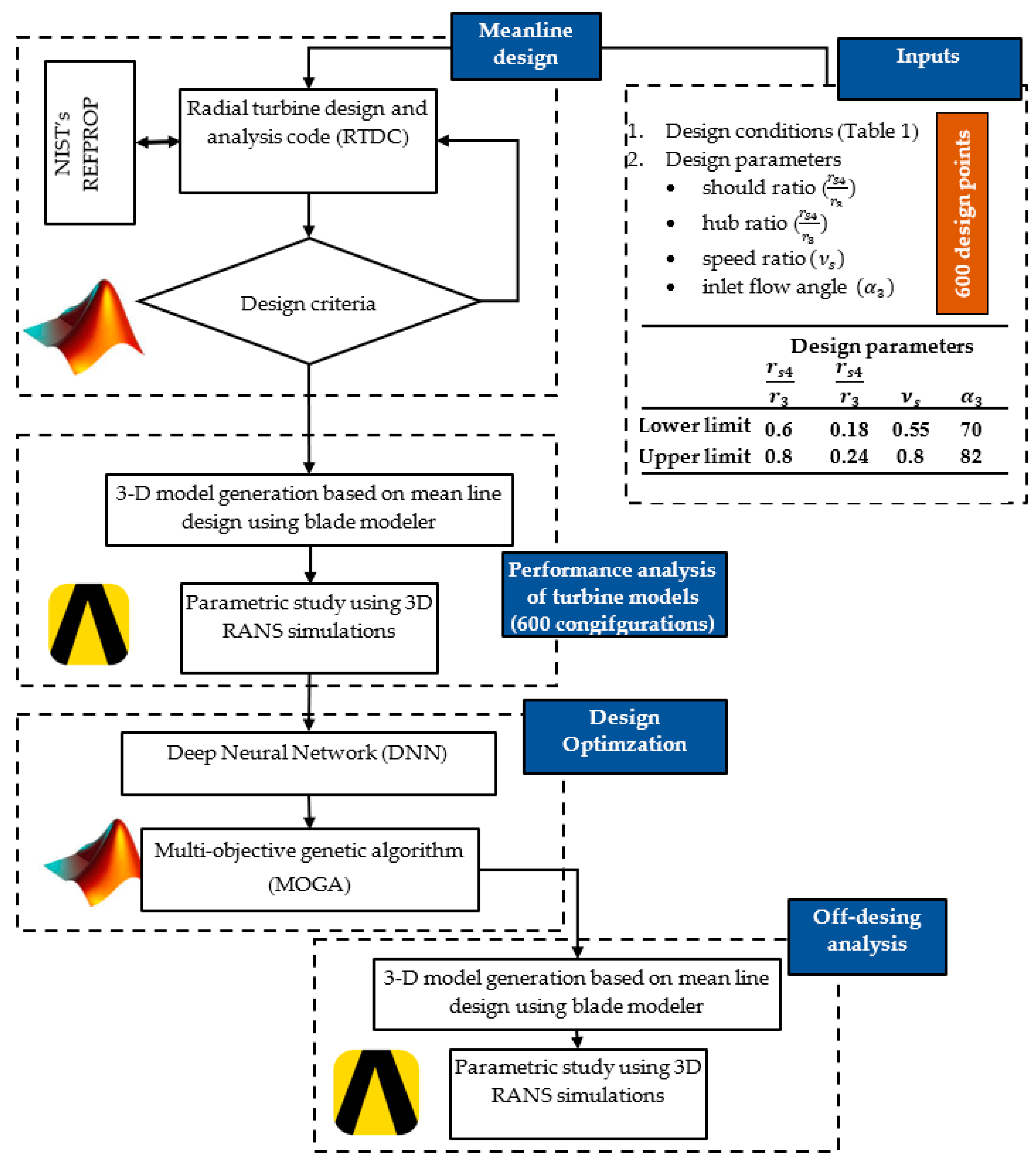
2. Methodology

The present study involves optimization of the radial turbine for an 8 MW sCO₂-BC turbine. The section gives a complete layout of the methodology adopted. A base design of the turbine is computed using in-house radial turbine design and analysis code (RTDC), and later geometry of the turbine is varied by changing the selected turbine design geometric parameters, i.e., $\frac{r_{s4}}{r_3}, \frac{r_{s4}}{r_3}, {\nu }_s$ and ${\alpha }_3$ (Section 1). The range of these design parameters is shown in Figure 1. Six hundred sets of turbine geometries are calculated using RDTC (Section 3) and analyzed numerically through 3D-RANS simulations (Section 4). A machine learning model based on the deep neural network (DNN) is trained using 600 data sets (Supplementary Table S1). The trained DNN model is used as a fitting function in the multi-objective genetic algorithm (MOGA) to explore the optimized design parameters for the rotor geometry. Finally, the off-design performance of the optimized turbine geometry is computed and reported. A flow chart of the methodology followed in the current study is shown in Figure 1.

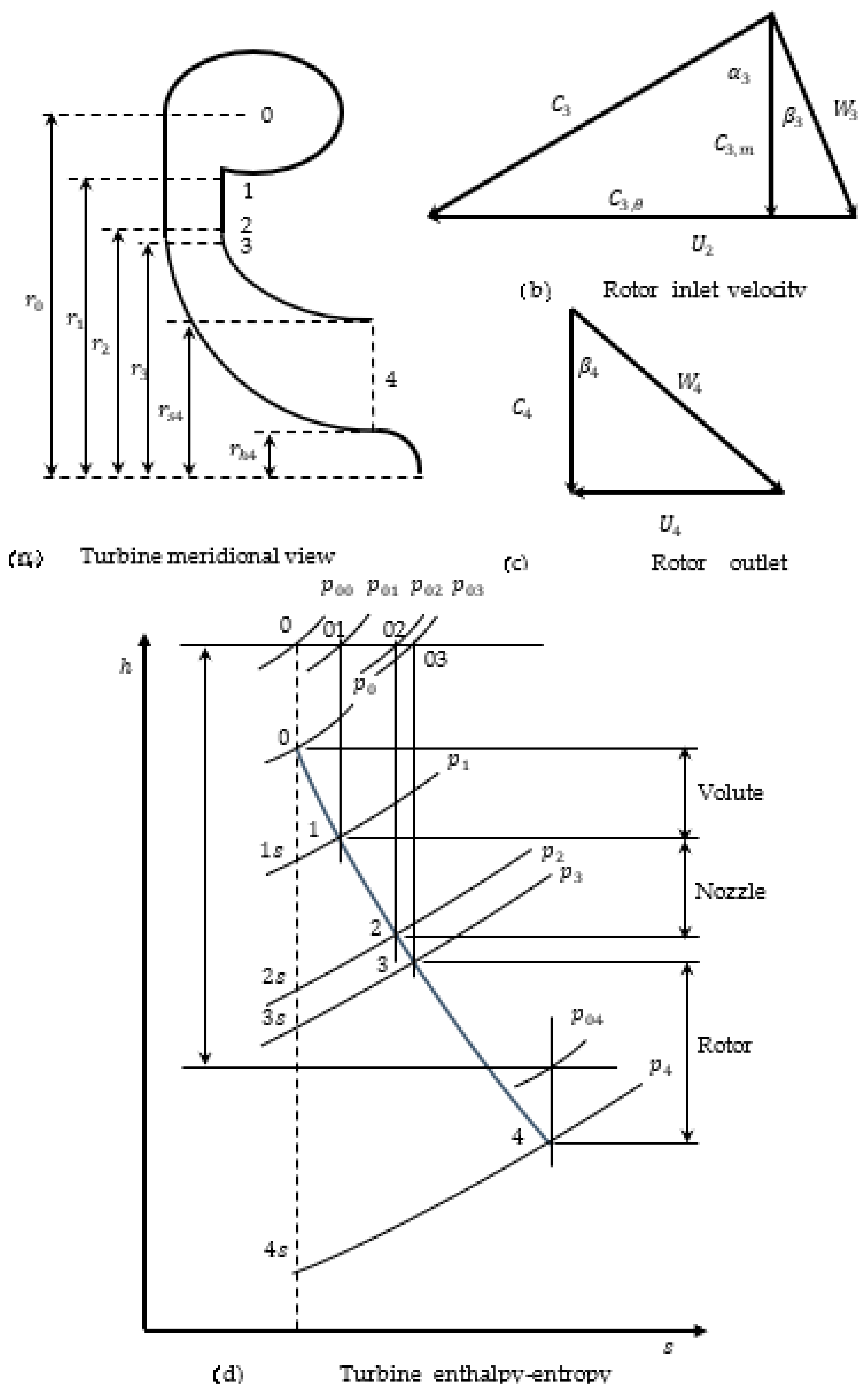
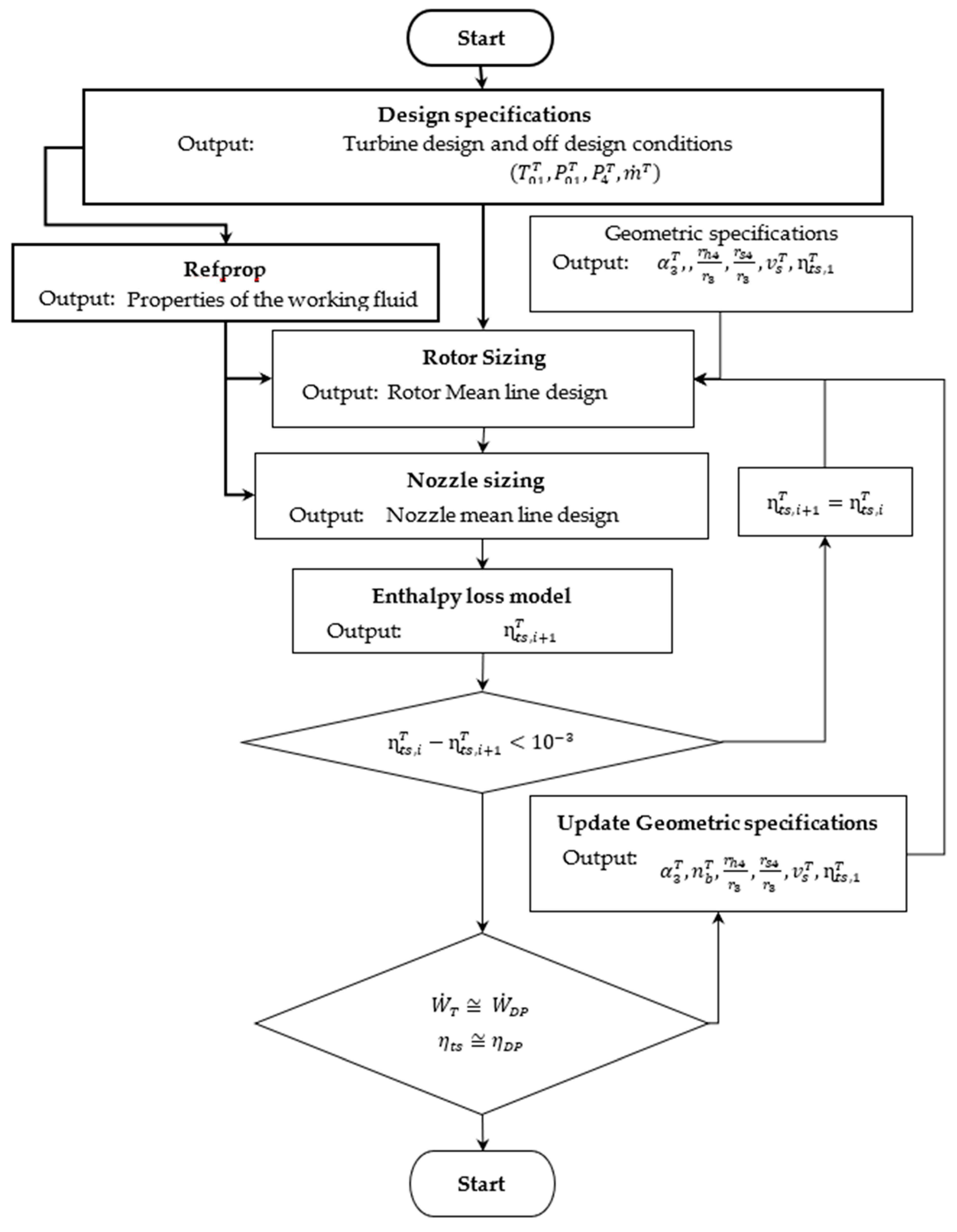
3. Meanline Design Procedure

The Radial turbine system comprises three sub-modules as shown in Figure 2:

• Volute (0–1): dispenses the flow evenly to each blade passage and converts pressure head to velocity head to some extent.
• Nozzle (1–2): converts pressure head to velocity head and aligns the flow with the rotor at the required angle.
• Rotor (3–4): the kinetic energy of the working fluid is transformed into mechanical work.

3.1. Radial Turinbe Rotor Desing Code (RTRDC)

The current section explains the one-dimensional mean line design model on which radial turbine rotor design code (RTRDC) is developed.

The base design for the turbine rotor is calculated applying a 1-D mean line design approach [23,24] for the design conditions listed in

Table 1. Given and required conditions for the design of the Expander system.

Items	Symbols	Values
The mass flow rate of exhaust CO2	$\dot{m}$	50 [kg s−1]
Temperate of exhaust gases	$T_{o1}$	983 [K]
Expansion ratio	$\frac{P_{o1}}{P_3}$	3
The desired value of total to static efficiency	${ŋ}_{ts}$	0.90
Desired turbine output power	$\dot{W}$	8 [MW]
Rotational speed	ω	40,000 [rpm]

. Mass flow rate of CO₂ ($\dot{m})$, exhaust gases temperature and pressure that will be used as inlet temperature ($T_{o1}$), and inlet pressure of the turbine ($P_{o1}$), using exit condition as the ambient condition, can be calculated from the information in Table 1. With the above given known information, the specific speed ($N_s^T)$ of the turbine can be approximated using Equation (1). $N_s^T$. The thermophysical properties of CO₂ [25,26] at all other points (1,2,3,4) are calculated using REFPROP [27] by coupling it with the RTDC.

$$N_s^T=\frac{\omega \sqrt{Q_4}}{{\left(\Delta H_{id}\right)}^{0.75}}$$

(1)

The term $Q_4$ = ${\dot{m}}_4^T/{\rho }_{04}^T$ is estimated by computing the ${\rho }_{04}^T$ based on the turbine exit conditions. It is to be noted here that the turbine exit conditions in this study will be ambient conditions. Value of $\Delta h_{0,idl}^T$ is calculated through REFPROP by using the available values, i.e.,$h_{04}^T,$ $s_{01}^T$ and $p_4^T$. The design process starts by providing the designs specifications, i.e., static velocity ratio ($v_{ts}^T$), desired total to static efficiency (${\mathsf{ŋ}}_{ts}^T$) and absolute flow angle at the rotor’s inlet (${\alpha }_3^T$). These specifications are described using relations given in Equations (2)–(4), where the limits adopted for these design variables are provided in

Table 2. Mesh optimization study.

Mesh	Number of Nodes in Streamwise Direction					Span Wise Direction		Theta Direction	CPU Time/10 Iterations [s]	Memory Consumed [MB]	${\mathit{\eta }}_{\mathit{t}\mathit{s}}$
	Inlet Domain	Nozzle Blade	Nozzle Rotor Gap	Rotor Blade	Outlet Domain	Along with Blade	Tip Clearance Region
M1	25	35	20	45	25	70	11	45	318	5612	82.32
M2	35	40	25	55	35	80	15	65	672	9653	87.57
M3	40	50	30	70	40	90	19	85	1548	2578	91.31
M4	50	60	35	80	50	100	23	95	2347	3517	91.19

.

$$v_s^T=0.737 N_{ts}^{0.2}$$

(2)

$${\mathsf{ŋ}}_{ts}^T=0.87-1.07{\left(N_s^T-0.55\right)}^2-0.5{\left(N_s^T-0.55\right)}^3$$

(3)

The discharge spouting velocity ($C_{0s}^T$) is calculated using Equation (4), while the rotor speed is assessed utilizing Equation (5). Conversely, the stagnation enthalpy ($h_{04}^T$) is calculated employing efficiency

$$C_{0s}^T=\sqrt{2\Delta H_{idl}}$$

(4)

$$U_3^T=v_s^T{C}_{0s}^T$$

(5)

$$h_{04}^T=h_{01}^T-\Delta h_{0,idl}^T{\mathsf{ŋ}}_{ts}^T$$

(6)

Once the $U_3^T$ is available, Equation (7) can be used to find the inlet rotor radius ($r_3^T$). The value of $P_{03}^T$ is calculated using Equation (8) [23]. It is to be noted here that the value of ${\rho }_{01}^T$ can be calculated obtained as a function of $T_{01}^T$ and ${\rho }_{01}^T$ utilizing REFPROP. Once the values of $C_{\theta 3}^T$, ${\alpha }_3^T$, and $U_3^T$ are available, the inlet velocity triangle is completed. Apart from the number of blades ($n_b^T)$, thickness of blade at inlet $t_{b3}^T$ and outlet ($t_{b4}^T)$, $r_{h4}^T$, and $r_{s4}^T$ cane be projected applying Equations (11)–(14).

$$r_3^T=U_3^T/\omega$$

(7)

$$P_{03}^T=P_{01}^T-\frac{{\rho }_{01}^T\Delta h_{0,idl}^T\left(1-{\eta }_s^T\right)}{4}$$

(8)

$$C_{\theta 3}^T=\frac{U_3^T {\eta }_s^T}{ 2{v_s^T}^2}$$

(9)

$$n_b^T=\frac{\pi }{30} \left( 110-{\alpha }_3^T\right)\tan {\alpha }_3^T$$

(10)

$$t_{b3}^T=0.04 r_3^t$$

(11)

$$t_{b4}^T=0.02 r_3^T$$

(12)

$$r_{h4}^T=0.22 r_3^T$$

(13)

$$r_{s4}^T=0.7 r_3^t$$

(14)

To calculate the inlet value of the passage width ($b_3^T$), enthalpy ($h_3^T$) is estimated via already computed values of $h_{03}^T$ and $C_3^T$ Using Equation (15). Additionally, $s_{03}^T$ is calculated using REFPROP from the known values of $P_{03}^T$ and $h_{03}^T$. Now considering $s_{03}^T=s_3^T$, the quantities $p_3^T$, $T_3^T, {\rho }_3^T$ and ${\mu }_3^T$ can be calculated through REFPROP using know values of $h_3^T$ and $s_3^T$. Now, the value of the $b_3^T$ can be estimated utilizing Equation (15).

At first, the value of ${\rho }_4^T$ is guessed and $C_{m4}^T$ is estimated applying Equation (16). considering the fact $r_4^t=\frac{\left(r_{sh4}^T+r_{h4}^T\right)}{2}$ and $b_4^T=\left(r_{sh4}^T-r_{h4}^T\right)$. Now $h_4^T$ can be calculated using Equation (17). using available values of $h_{04}^T$ from Equation (6) and ${\rho }_4^T$ is adjusted applying REFPROP as function of $h_4^T$ and $p_4^T$ adopting an iterative process. With corrected value of ${\rho }_4^T$, all remaining quantities can be estimated using REFPROP using know values of ${\rho }_4^T$ and $p_4^T$. Once all above quantities are known, nozzle dimension, $r_2^T$ can be calculated utilizing Equation (18). [28], where the $r_1^T$ is obtained using a ratio $\frac{r_1^T}{r_2^T}=1.3$ [24].

$$b_3^T=\frac{{\dot{m}}^T}{2 \pi r_3^T{\rho }_3^T{C}_{m3}^T}$$

(15)

$$C_{m4}^T=\dot{\frac{m^T}{2\pi r_4^T{b}_4^T{\rho }_4^T}}$$

(16)

$$h_4^T=h_{04}^T-\frac{1}{2}{C}_{m4}^T.$$

(17)

$$r_2^T=r_3^T+2b_3^T\cos {\alpha }_4^T.$$

(18)

3.2. Efficiency Correction

The rotor sizing computed in the previous step is built on an imagined value of the ${\mathsf{ŋ}}_{ts}^T$. The value of ${\mathsf{ŋ}}_{ts}^T$ is be corrected through an interactive process displayed in Figure 3, where the corrected efficiency values ${\mathsf{\eta }}_{\mathrm{ts}}^{corrected,T}$ using estimated values of the total losses $\Delta h_{loss}^T$, available in Equation (20). $\Delta h_{loss}^T$ is the sum of passage losses ($\Delta h_{passage}^T)$, tip clearance losses ($\Delta h_{tip clearance}^T)$, exit losses ($\Delta h_{exit}^T)$ and nozzle losses $\Delta h_{nozzle}^T$ using information available in Equations (21)–(33). Missing aspects on the loss model are variable in the authors earlier work [29].

$${\mathsf{\eta }}_{\mathrm{ts}}^{corrected,T}=\frac{\Delta h_{loss}^T}{\Delta h_{loss}^T+\Delta h_{actual}^T}$$

(19)

$$\Delta h_{loss}^T=\Delta h_{passage}^T+\Delta h_{tip clearance}^T+\Delta h_{exit}^T+\Delta h_{nozzle}^T$$

(20)

$$\Delta h_{passage}^T=K_{passage}\left\{\left(\frac{l_{hyd}^T}{d_{hyd}^T}\right)+0.68\left[1-{\left(\frac{r_4^T}{r_3^T}\right)}^2\right]\frac{cos{\beta }_4^T}{\frac{b_4^T}{c}} \right\} 0.5\left(W_3^{2,T}+W_4^{2,T}\right)$$

(21)

where

$$l_{hyd}^T=\frac{\pi }{4}\left[\left(𝓏-\frac{b_3^T}{2}\right)+\left(r_3^T-r_{s4}^T-\frac{b_4^T}{2}\right)\right]$$

(22)

$$d_{hyd}^T=\frac{1}{2}\left[\left(\frac{4\pi r_4^T{b}_3^T}{2\pi r_3^T+n_b^T{b}_3^T}\right)+\left(\frac{2\pi \left(r_{s4}^{2,T}-r_{h4}^{2,T}\right)}{\pi \left(r_{s5}^T-r_{h5}^T\right)+n_b^T{b}_4^T}\right)\right]$$

(23)

$$c=\frac{𝓏}{\cos \overline{\beta }} \mathrm{where} \tan \overline{\beta }=\frac{1}{2}\left(\tan {\beta }_3^T+\tan {\beta }_4^T\right)$$

(24)

$$\Delta h_{tip clearance}^T=\frac{U_3^{3,T}{n}_b^T}{8\pi }\left(0.4 {\epsilon }_x^T{C}_x^T+0.75{\epsilon }_r^T{C}_r^T-0.3\sqrt{{\epsilon }_x^T{\epsilon }_r^T{C}_x^T{C}_r^T}\right)$$

(25)

where

$$C_x^T=\frac{1-\left(\frac{r_{s4}^T}{r_3^T}\right)}{C_{m3}^T{b}_3^T} ,C_r^T=\left(\frac{r_{s4}^T}{r_3^T}\right)\frac{𝓏-b_4^T}{C_{m6}^T{r}_4^T{b}_3^T}$$

(26)

$${\epsilon }_x^T={\epsilon }_r^T=0.02\left(r_{s4}^T-r_{h4}^T\right)$$

(27)

$$\Delta h_{exit}^T=\frac{1}{2} C_4^{2,T}$$

(28)

$$\Delta h_{nozzle}^T=4f_{nozzle}^T \overline{C}\frac{l_{hyd,nozzle}^T}{d_{hyd,nozzle}^T}$$

(29)

where

$$R{e}_{nozzle}^T=\frac{\frac{U_1^T{b}_3^T{\rho }_1^T}{{\mathsf{\mu }}_1^T}+\frac{U_2^T{b}_3^T{\rho }_2^T}{{\mathsf{\mu }}_1^T}}{2}$$

(30)

$$f_{nozzle}^T=8{\left[{\left(\frac{8}{R{e}_{nozzle}^T}\right)}^{12}+{\left({\left[2.457\ln \left(\frac{1}{{\left(\frac{7}{R{e}_{nozzle}^T}\right)}^{0.9}+0.27 RR}\right)\right]}^{16}+{\left[\frac{37530}{R{e}_{nozzle}^T}\right]}^{16}\right)}^{-1.5}\right]}^{\frac{1}{12}}$$

(31)

$$l_{hyd,nozzle}^T=r_1^T-r_2^T$$

(32)

$$d_{hyd,nozzle}^T=\frac{1}{2}\left[\frac{8\pi r_1^T{b}_3^T\cos \left({\alpha }_1^T\right)}{4\pi r_1^T+\frac{4\pi b_3^T{r}_1^T}{\sigma }}+\frac{8\pi r_2^T{b}_3^T\cos \left({\alpha }_2^T\right)}{4\pi r_2+\frac{4\pi b_3^T{r}_2^T}{\sigma }}\right]$$

(33)

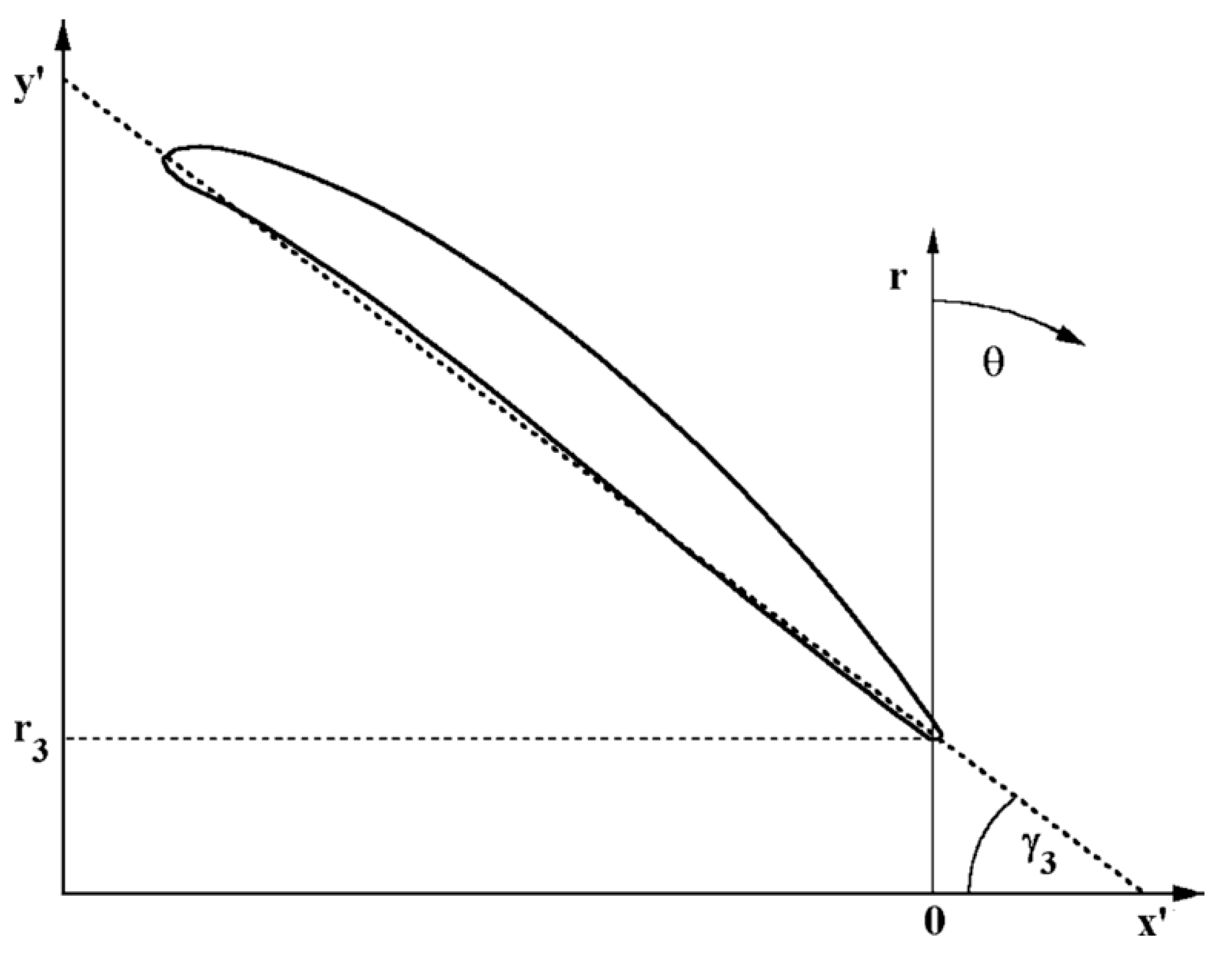
3.3. Nozzle Geometry

Because the flow is not supersonic at the blade trailing edge when the machine is operating at the design point, the blade angle of the nozzle vane is set to be the same as the rotor inlet absolute flow angle asa shown in Figure 4.

$${\beta }_1={\beta }_2={\alpha }_3$$

(34)

The blade height at the inlet and outlet of the nozzle is assumed to be equal to the rotor inlet blade height as given by Equation (35).

$$b_1=b_2=b_3$$

(35)

Watanabe et al. [28] introduced a correlation to estimate a suitable distance for this gap, as given by Equation (36)

$$\Delta r^T=2. b_3 .\cos {\alpha }_3$$

(36)

Thus, the radius at the nozzle exit can be calculated from Equation (37)

$$r_2^T=r_3^T+\Delta r^T$$

(37)

The tangential component of absolute velocity at nozzle outlet is defined by Equation (38) given below.

$$C_{\theta 2}=C_{\theta 3}\frac{r_3}{r_2}$$

(38)

Meridional component of absolute velocity at nozzle outlet is computed using Equation (39)

$$C_{m2}=\frac{C_{\theta 2}}{\tan {\alpha }_2} \mathrm{where} {\alpha }_2={\alpha }_3$$

(39)

Once all parameters above are established, the absolute velocity at the nozzle outlet could be computed using the equation below.

$$C_2=\sqrt{{\left(C_{\theta 2}\right)}^2+{\left(C_{m2}\right)}^2}$$

(40)

Because the nozzle inlet conditions are unknown, an approximate equation suggested by Augier [23] is used to estimate the meridional component of absolute velocity at the nozzle inlet. The inlet absolute flow angle is assumed. Augier suggested that the ratio of nozzle inlet to outlet radius lies between 1.1 and 1.7. Value is set to 1.2 of this case; thus, using $r_1^T=1.2r_2^T$, $C_{m1}$ is finalized using iterative method given by Equation (41).

$$\begin{gathered} C_{m1 }=C_{m2} ,\frac{r_3}{r_2} \mathbf{\to } C_{\theta 1}=C_{m1}\tan \alpha 1 \mathbf{\to } C_1=\sqrt{{\left(C_{\theta 1}\right)}^2+{\left(C_{m1}\right)}^2} \\ \mathrm{Now}, H_1=H_{01}-\frac{1}{2} C_1^2 \\ \mathrm{Update} \mathrm{meridional} \mathrm{component} \mathrm{of} \mathrm{absolute} \mathrm{velocity} \mathrm{at} \mathrm{nozzle} \mathrm{inlet}: \\ {C}_{m1}=\dot{\frac{m}{2\pi r_1{b}_1{\rho }_1}} \end{gathered}$$

(41)

The updated $C_{m1}$ is used iteratively until the results converge.

The blade shape is computed using Equation (42)

$$x^2+\frac{c-2a}{b} xy+\frac{{\left(c-2a\right)}^2}{4b^2} y^2-cx-\frac{c^2-4ac}{4b}y=0$$

(42)

This could be converted to a recursion equation

$$y=\frac{x\left(c-x\right)}{\frac{{\left(c-2a\right)}^2}{4b^2} y+\frac{c-2a}{b} x-\frac{c^2-4ac}{4b}}$$

(43)

The blade thickness distribution is adapted from a distribution used by Augier [23] for return channel vanes, as shown in Nomenclature of a typical airfoil geometry, the maximum blade thickness, $t_{max}$, and its location, $d$, are specified along with the leading and trailing edge blade thicknesses. A “nose radius” is imposed at each end of the camber line using Equation (45).

$$\begin{gathered} t=t_{ref}+\left[t_{max}-t_{ref}\right]{\xi }^e \\ \mathrm{where} \\ {t}_{ref}=t_2+\left[t_3-t_2\right]\left(\frac{x}{d}\right) \\ \xi =\frac{x}{d}; x\le d \\ \xi =\frac{c-x}{c-d}; x>d \\ e=\sqrt{\frac{0.4d}{c}} \left[0.95\left(1-\frac{x}{c}\right)\left(1-\xi \right)+0.05\right] \end{gathered}$$

(44)

Now the profiles coordinate of the profile could be computed using the following equation.

$$\begin{gathered} x=x_c\pm \frac{1}{2}t\sin \chi \\ y=y_c\mp \frac{1}{2}t\sin \chi \end{gathered}$$

(45)

The normalized airfoil geometry (Figure 5) can be used to define the nozzle blade by determining the chord and the nozzle setting angle, ${\gamma }_3$ given by Equation (46).

$$\begin{gathered} x^{\prime }=\left(x-c\right)sin{\gamma }_3+ycos{\gamma }_3 \\ {y}^{\prime }=r_3-\left(x-c\right)sin{\gamma }_3+ycos{\gamma }_3 \end{gathered}$$

(46)

While corresponding polar coordinates are

$$\begin{gathered} r=\sqrt{x^{\prime 2}+y^{\prime 2}} \\ \tan \theta =\frac{x^{\prime }}{y^{\prime }} \end{gathered}$$

(47)

4. CFD Model

The current problem is solved using the RANS equation and the Equations (48)–(50) [24,27] using the commercial code ANSYS-CFX.

$$\nabla .\rho \mathrm{V}=0$$

(48)

$$\nabla .\left(\rho \mathrm{V}\otimes \mathrm{V}\right)=-\nabla p+\nabla .\mathsf{\tau }$$

(49)

For turbulent flow, the stress tensor (τ) is defined in Equation (50).

$$\mathsf{\tau }=\left(\mu +{\mu }_t\right)\left(\nabla \mathrm{V}+{\left(\nabla \mathrm{V}\right)}^T-\frac{2}{3}\delta \nabla .\mathrm{V}\right)=\mu \left(\nabla \mathrm{V}+{\left(\nabla \mathrm{V}\right)}^T-\frac{2}{3}\delta \nabla .\mathrm{V}\right)+\nabla .\mathsf{\Pi }$$

(50)

Geometrical Model and Mesh

ANSYS blade modeler is utilized to generate the 3D model of the turbine rotor and nozzle guide vane (Figure 6). Later, the model is exported to ANSYS Turbo Grid, where structured mesh of the rotor and nozzle guide vane was generated. The mesh of the rotor and nozzle guide vane is show in Figure 6. Mesh in the boundary layer region was generated using the guidelines that can be found in previous work of the authors [30,31]. To find the optimized mesh size and node distribution, four, namely M1, M2, M3, and M4, generated details on which are listed in Table 2 and shown in Figure 6. The parameters, i.e., efficiency value of the turbine (${\eta }_{ts})$, memory consumed, and computational time, were used in the selection of optimized mesh for the current study. It is evident from the data listed in Table 2 that Mesh M3 and M4 resulted in the same value of the ${\eta }_{ts}$; however, the computational time and memory used by the mesh M3 are substantially lower that M4. In view of the above finding, mesh M4 is selected as an optimized mesh.

5. Machine Learning Model

In this section, the details of the developed machine learning model (ML) to be trained on the radial turbine design data are presented.

5.1. Training Data Details

As described in Section 1 (Methodology), data used to train the machine learning model is computed using 3D RANS simulations. The ML model opted for the current work is deep neural network (DNN) that is trained using data comprises 600 data sets. Each dataset consists of four input variables ($\frac{r_{s4}}{r_3}, \frac{r_{s4}}{r_3}, {\nu }_s, {\alpha }_3)$, and two output parameters (${\eta }_{ts}$ and $r_3$), as displayed in

Table 3. Details of the input and output variables.

	Input Parameters				Output Parameter
S. No.	${\mathit{r}}_{\mathit{s}\mathbf{4}}/{\mathit{r}}_{\mathbf{3}}$	${\mathit{r}}_{\mathit{s}\mathbf{4}}/{\mathit{r}}_{\mathbf{3}}$	${\mathbf{\nu }}_{\mathit{s}}$	${\mathbf{\alpha }}_{\mathbf{3}}$	${\mathbf{\eta }}_{\mathit{t}\mathit{s}}$	${\mathit{r}}_{\mathbf{3}} \left[mm\right]$
1	0.6	0.18	0.55	70	0.77	161.71
2	0.6	0.18	0.55	73	0.78	161.71
3	0.6	0.18	0.55	76	0.78	161.71
4	0.6	0.18	0.55	79	0.79	161.71
5	0.6	0.18	0.55	82	0.79	161.71
6	0.6	0.18	0.6	70	0.82	176.41
7	0.6	0.18	0.6	73	0.83	176.41
8	0.6	0.18	0.6	76	0.83	176.41
.	.	.	.	.	.	.
.	.	.	.	.	.	.
.	.	.	.	.	.	.
600	0.8	0.24	0.8	82	0.82	270.49

.

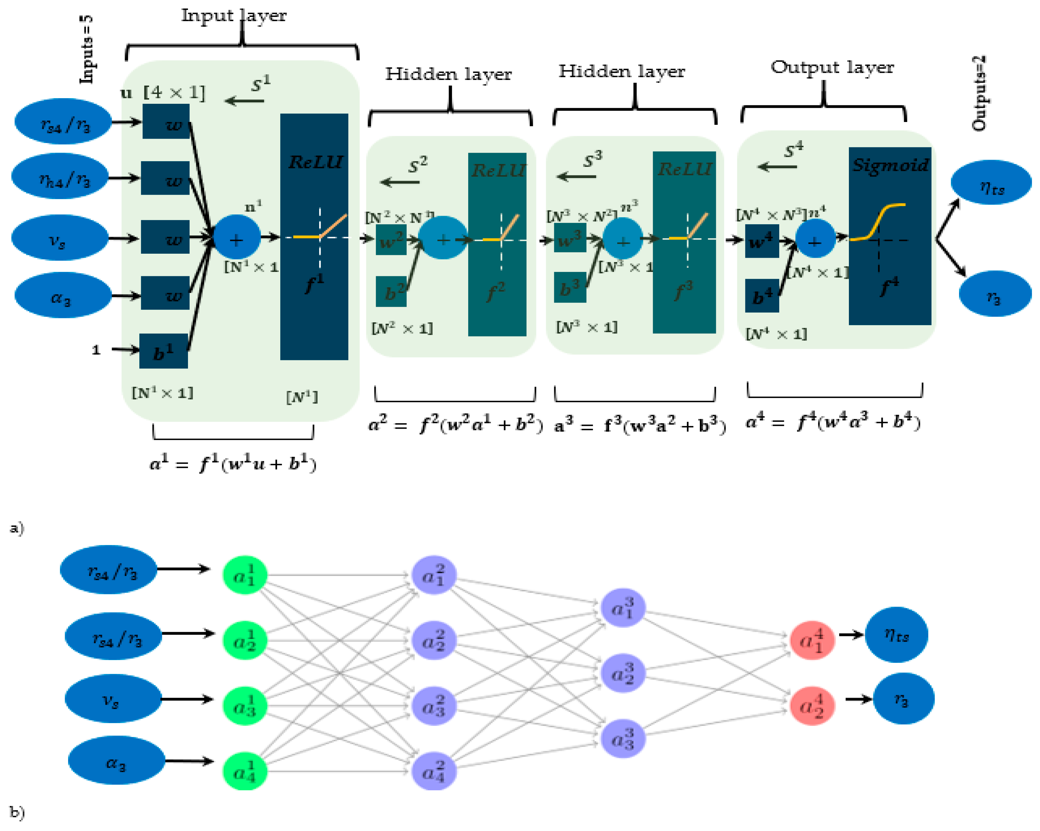
5.2. The Deep Neural Network

A deep neural network (DNN) is developed for training the ML model, as the structure and hyperparameters of DNN are observed appropriate for problems identical to those studied in the current work [32].

The composition of the DNN is to push the data back and forth iteratively, where weights and biases are adjusted through some optimizing function, as shown in Figure 7a. The figure explicates the construction of the DNN with an input, two hidden, and an output layer. All the hyperparameters connected with the deep neural network (DNN), i.e., number of hidden layers, neurons in each layer, activation function, and optimization function), were finalized to obtain a minimum value of the root mean square (RSM) error. Further details on the model can be found in the author’s previous work [33,34,35]. The current DNN model is finalized with two hidden layers consisting of four and three neurons in the first and second layers, respectively, with Levenberg–Marquardt (LM), as an optimizing algorithm; Rectifier Linear Unit (ReLU) as an activation function for the input and the two hidden layers, and sigmoid as an activation function for the output layer as displayed in Figure 7.

The input layer symbolizes the neuron with the normalized data, while the data from $i\mathrm{th}$ layer to $i+1\mathrm{th}$ move as described by Equation (51).

$${\mathrm{a}}_q^{i\to i+1}={ \mathrm{f}}_q^i\left({\displaystyle \sum }_{p=1}^{N^i}{\mathrm{w}}_{qp}^i{\mathrm{L}}_{\mathrm{p}}^i+{\mathrm{b}}_q^i\right)$$

(51)

where the term q varies from 1 to $N^{i+1}$ The above equation 1 can be expressed in the vector format as given by Equation (52).

$$a^{i+1}=f^i\left(w^i{a}^i-1+b^{i+1}\right)$$

(52)

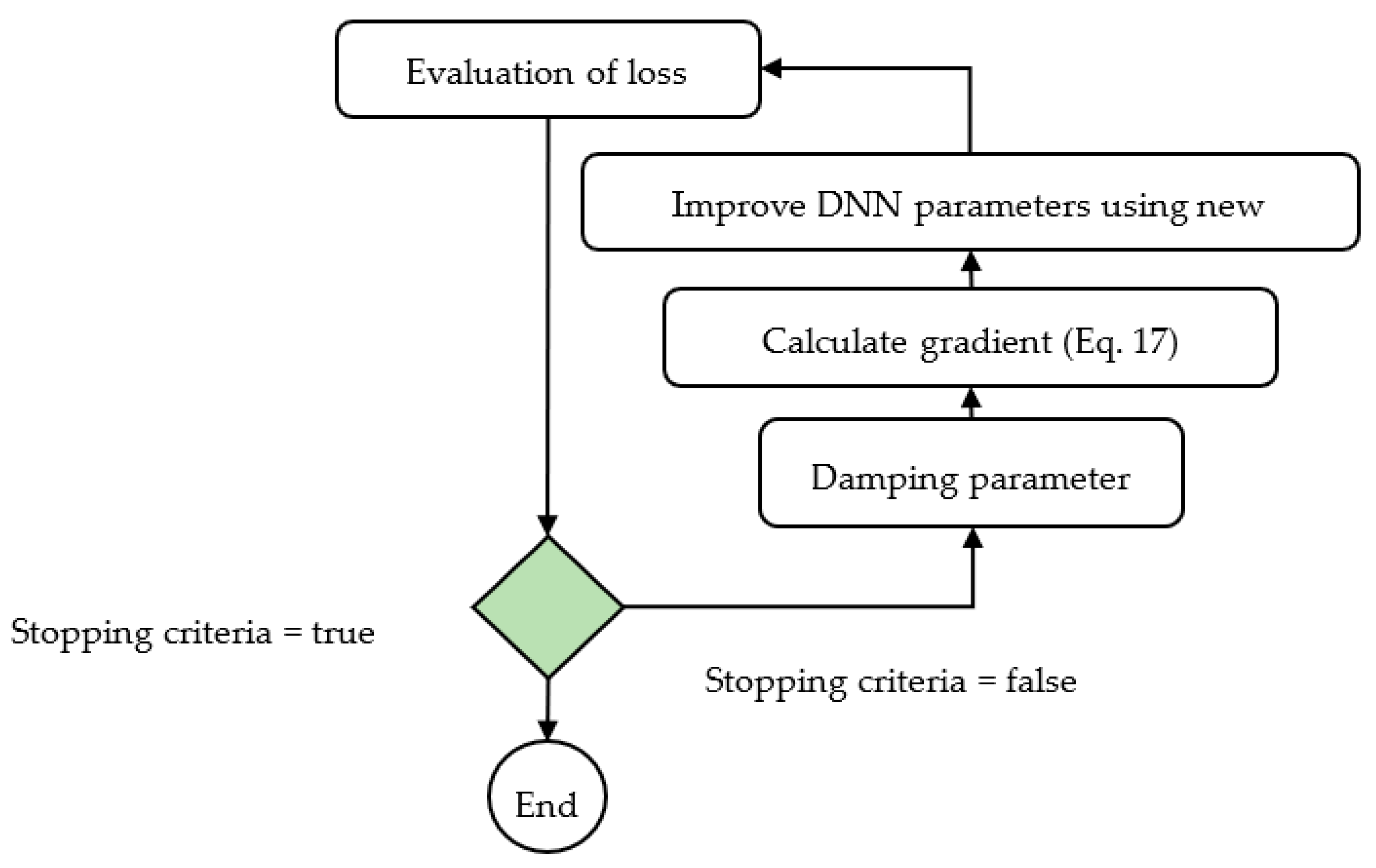
DNN Optimization Methodology

Executing a deep neural network (DNN) learning activity is recognized as an optimizer or optimization algorithm. Among several optimizers available for deep neural network, Levenberg–Marquardt (LM) algorithm is utilized for the current work.

The learning process of LM algorithm is explained by Equation (53), and Figure 8.

$$w^{\left(i+1\right)}=w^{\left(i\right)}-{\left(J^{\left(i\right)T}.J^{\left(i\right)T}+{\mathsf{\lambda }}^{\mathrm{i}}I\right)}^{-1}. 2J^{\left(i\right)T}.e^{\left(i\right)})$$

(53)

The quantity λ and J are the damping factor and Jacobian matrix in the above term.

The Jacobian matrix is characterized by Equation (54).

$$J_{i,j}=\frac{\partial e_i}{\partial w_j} \mathrm{for} i=1,\dots ,m; \mathrm{and} j=1,\dots ,n$$

(54)

6. Optimization of the Turbine Geometry

The geometry of the turbine rotor is optimized by exploiting the trained machine learning model (Section 5) as a fitness function of a multi-objective genetic algorithm (MOGA). Four variables, i.e., $\frac{r_{s4}}{r_3}, \frac{r_{s4}}{r_3}, {\nu }_s$ and ${\alpha }_3$, are used as design parameters in the optimization process, while turbine efficiency and rotor radius are used objective function. The limits of the design variables used for the turbine optimization study are shown in

Table 4. Adopted limits of the design variables.

	Design Parameters				Objective Function
	${\mathit{r}}_{\mathit{s}4}/{\mathit{r}}_3$	${\mathit{r}}_{\mathit{s}4}/{\mathit{r}}_3$	${\mathit{\nu }}_{\mathit{s}}$	${\mathit{\alpha }}_3$	${\mathit{\eta }}_{\mathit{t}\mathit{s}}$	${\mathit{r}}_3$
Lower limit	0.6	0.18	0.55	70	Maximize	Minimize
Upper limit	0.8	0.24	0.8	82

, where turbine efficiency is set to maximize, and rotor radius is minimized.

The diagram of the approach chosen for the utilized optimization problem is demonstrated in Figure 9. The process starts with an arbitrary initialization of a specified population size of 100 sequences of the input parameters. The engendered population is then analyzed by the fitness function (trained ML model) for the specified objective function (rotor size and efficiency). Further aspects of the GA are available in the literature [36,37,38].

7. Results

Figure 10 shows the sensitivity analysis of the turbine’s performance parameters to the turbine’s design parameters. It is to be noted here that the length of the bar will show the level of sensitivity independent of the negative or positive signs. Negative values only show the inverse relationship between the performance parameters and design parameters. Hence, it can be observed from the Figure that all turbine’s performance parameters shown in Figure 10 (power, efficiency, various types of losses, rotor radius, and impellor length) are most sensitive to the speed ratio (${\nu }_s$) followed by the inlet flow angle (${\alpha }_3$). At the same time, the turbine’s performance is found least sensitive to the turbine’s hub ratio.

As mentioned above, the data computed using the 3D-RANS simulations are used to train the deep neural network (DNN). Various combinations of the hyperparameters are used, and the combination corresponding to the maximum performance is finalized. The Levenberg–Marquardt (LM) is finalized as an optimizer for DNN with two hidden layers; the first consists of four neurons, and the second involves three neurons. Seventy percent of the total data is used for the training, where 15% of data is utilized for testing and validation purposes. It is to be noted here that 10-fold cross-validation is utilized while training the deep neural network.

Figure 11 illustrates the mean squared error (mse) plotted the number of occurrences again out of entire data sets, i.e., 600. The data in the Figure reflect that training error is almost negligible for the selected hyperparameters of DNN. Figure 12 shows R-values for the validation, testing, and training data sets. It can be observed that R values for all data are 0.99. This demonstrates that the trained model can predict 99% of the generated data among all data sets. Simultaneously, the ability of the trained DNN to approximate individual percentage variability for training, validation, and test data are almost identical, reflecting the model is not overfitting the data.

Figure 13 shows the effect of the design parameter on the turbine performance parameters. Figure 13a shows that variation of turbines efficiency with the design parameters, i.e., $\frac{r_{s4}}{r_3},\frac{r_{s4}}{r_3},{\nu }_s$ and ${\alpha }_3$. Turbine efficiency increases substantially with the increase in the value of speed ratio $\left({\nu }_s\right)$ initially, attaining a maximum value and declining with further increases in the value of ${\nu }_s$. Conversely, the value of the turbine’s efficiency increases monotonically with inlet flow angle and shroud ratio and decreases slightly with hub ratio.

Figure 13b shows the effect of rotor inlet radius with the design parameter used in the current study. The only parameter that impacts the size of the rotor is the speed ratio. The rotor inlet radius changes significantly with the speed ratio. At the same time, the remaining three design parameters, namely, hub ratio, shroud ratio, and interflow angle, do not impact the rotor’s size noticeably. Figure 13c shows that variation of turbines impeller’s length with employed design parameter ($\frac{r_{s4}}{r_3},\frac{r_{s4}}{r_3},{\nu }_s$ and ${\alpha }_3$). The length of the impeller decreases markedly with the rise in the value of speed ratio $\left({\nu }_s\right)$ primarily, achieving a maximum value and falling with a further increase in the value of ${\nu }_s$. Conversely, the value of the turbine’s efficiency drops monotonically with inlet flow angle and shroud ratio. It rises marginally with the increase in the value of the hub ratio.

Figure 13d shows that exit losses of the turbine drop noticeably and non-linearly with speed ratio and hub ratio. However, it is to be noted here that exit losses are most sensitive to speed ratio. At the same time, exit losses increase slightly with the hub ratio and inlet flow angle to some extent. Figure 13e shows the effect of the design parameter on passage losses. Passage losses drop sharply with the speed ratio, but no significant effect of other design parameters is computed.

Figure 13f shows the impact of the design parameter on the nozzle losses. The nozzle losses decrease with the rise in the value of speed ratio $\left({\nu }_s\right)$ primarily, achieving a minimum value and then rising markedly with further increase in the value of ${\nu }_s$. Conversely, the value of the turbine’s nozzle losses does not change appreciably with inlet flow angle and hub ratio, and shroud ratio. The total losses of the turbine are plotted in Figure 13 with the design parameter ($\frac{r_{s4}}{r_3},\frac{r_{s4}}{r_3},{\nu }_s$ and ${\alpha }_3$) used in the current study. Total losses are most sensitive to the speed ratio. Total turbine losses drop sharply with ${\nu }_s$ until it reaches a minimum value and then starts rising at high values of ${\nu }_s$.

Figure 14 shows the response of the design parameters on the performance parameters used for the design optimization of the turbine’s rotor. Figure 14 displays that the value of the turbine’s efficiency increases with values of velocity ratio (${\nu }_s$) initially and then starts dropping after reaching a maximum value for all values of inlet flow angle $\left({\alpha }_3\right)$. However, the value of ${\nu }_s$ to which the peak value of the efficiency ($\eta )$ corresponds (referred as ${\nu }_{s,m}$) changes with the change in the value of the inlet flow angle ${\alpha }_3$. The value of the ${\nu }_{s,m}$ increases with the increase in the value of the inlet flow angle. Figure 14b shows the trends of the rotor’s size (rotor’s inlet diameter) increasing significantly with the increase in the value of the speed ratio but increasing marginally with the increase in the value of the ${\alpha }_3$. The results suggest that the value of ${\alpha }_3$ has no significant effect on the rotor sizing.

Figure 14c shows the response surface of the turbine’s efficiency bounded by the shroud ratio ($\frac{r_{s4}}{r_3}$) and hub ratio ($\frac{r_{h4}}{r_3})$. It can be observed that efficiency increases significantly with the increase in the value of $\frac{r_{h4}}{r_3}$ for all values of $\frac{r_{s4}}{r_3}$. Similarly, the value of the turbine’s efficiency increases with the increase in the value of $\frac{r_{s4}}{r_3}$ for all values of $\frac{r_{h4}}{r_3}$; however, the rise is much smaller in comparison with the increase linked with $\frac{r_{h4}}{r_3}$. Figure 14c shows the response surface of the turbine’s rotor radius ($r_3$) constrained by the shroud ratio ($\frac{r_{s4}}{r_3}$) and hub ratio ($\frac{r_{h4}}{r_3})$. It can be noted that $r_3$ rises appreciably with the growth in the value of $\frac{r_{h4}}{r_3}$ for all values of $\frac{r_{s4}}{r_3}$. Likewise, the value of the $r_3$ increase with the surge in the value of $\frac{r_{s4}}{r_3}$ for all values of $\frac{r_{h4}}{r_3}$, but the increase is tinier in comparison with the boost linked with $\frac{r_{h4}}{r_3}$.

As discussed above, to optimize the rotor’s geometry, the trained DNN was linked with the multi-objective genetic algorithm (MOGA). The list of the design variables and their rages are cataloged in Table 4. Figure 15 shows the Pareto front computed for rotor’s size and rotor’s efficiency using a multi-objective genetic algorithm. It is noted that by using the trained DNN and MOGA, the optimization process can be completed within 20–30 min. This suggests that the DNN-MOGA methodology is valuable during the optimization stages of the geometrical aspect for different computational fluid dynamics applications. Running over this huge range set of different design variables would consume an unrealistic amount of computational time. Therefore, by combining computational fluid dynamics with machine learning algorithms, more time and cost-efficient methods for design optimization can be achieved.

Figure 15 shows the Pareto front processed by coupling the trained DNN with a multi-objective genetic algorithm (MOGA), demonstrating the design parameters corresponding to the optimal geometries of the turbine rotor. Every point on the Pareto front symbolizes an optimal solution where the improvement in an objective function can be achieved at the second’s cost. If a designer intends on minimum rotor size values, region A will suit the desired condition. However, the values of the turbine’s efficiency $\left({\eta }_{ts}\right)$ corresponding to the design of region A are minimum among all optimized solutions. Simultaneously, if one is interested in higher values of the turbine’s efficiency with no trouble to higher values of the rotor’s size, region C would be appropriate under these situations. At the same time, region B corresponds to a good compromise between the value of the rotor’s size and its efficiency.

Despite the above discussion, it is to be noted here for sCO₂-BC that the size of the heat exchanger is much larger than its turbomachinery [4,39,40]. Therefore, the layout size of sCO₂-BC is dominated by PCHEs and marginally affected by the size of its turbomachinery. Therefore, it is recommended for sCO₂-BC to opt for the design of the turbine with higher efficiency, despite the fact it will increase the size of the turbine. Hence, the highlighted design in region B that corresponds to maximum efficiency is chosen for further analysis.

The turbine geometry with the parameters highlighted in region C was modeled in ANSYS blade modeler and analyzed using CFD for design and off-design conditions. Figure 16a shows the qualitative results of the pressure distribution on the hub and blades of the rotor and nozzle guide vane. Figure 16b shows the pressure distribution on the nozzle guide vane at 50% span, whereas Figure 16c shows the pressure distribution on the rotor’s blade at various span locations. Figure 17 displays the off-design performance of the optimized geometry. The off-design performance of the turbine is computed by changing the flow rates and rotational speed. Each point on the graph can be distinct by flow rate and rotations speed. It can be observed from the Figure that the off-design performance of the covers a wide range of the operating conditions. At the same time, both turbine’s efficiency and pressure ratio stay quite close to the design point performance with appreciable changes in the mass flow rate.

8. Conclusions

In the present study, a radial turbine design is constructed and optimized using a multifaceted technique that involves in-house code (RTDC), CFD, deep neural network, and multi-objective genetic algorithm (MOGA). The following deductions are made from the current investigation.

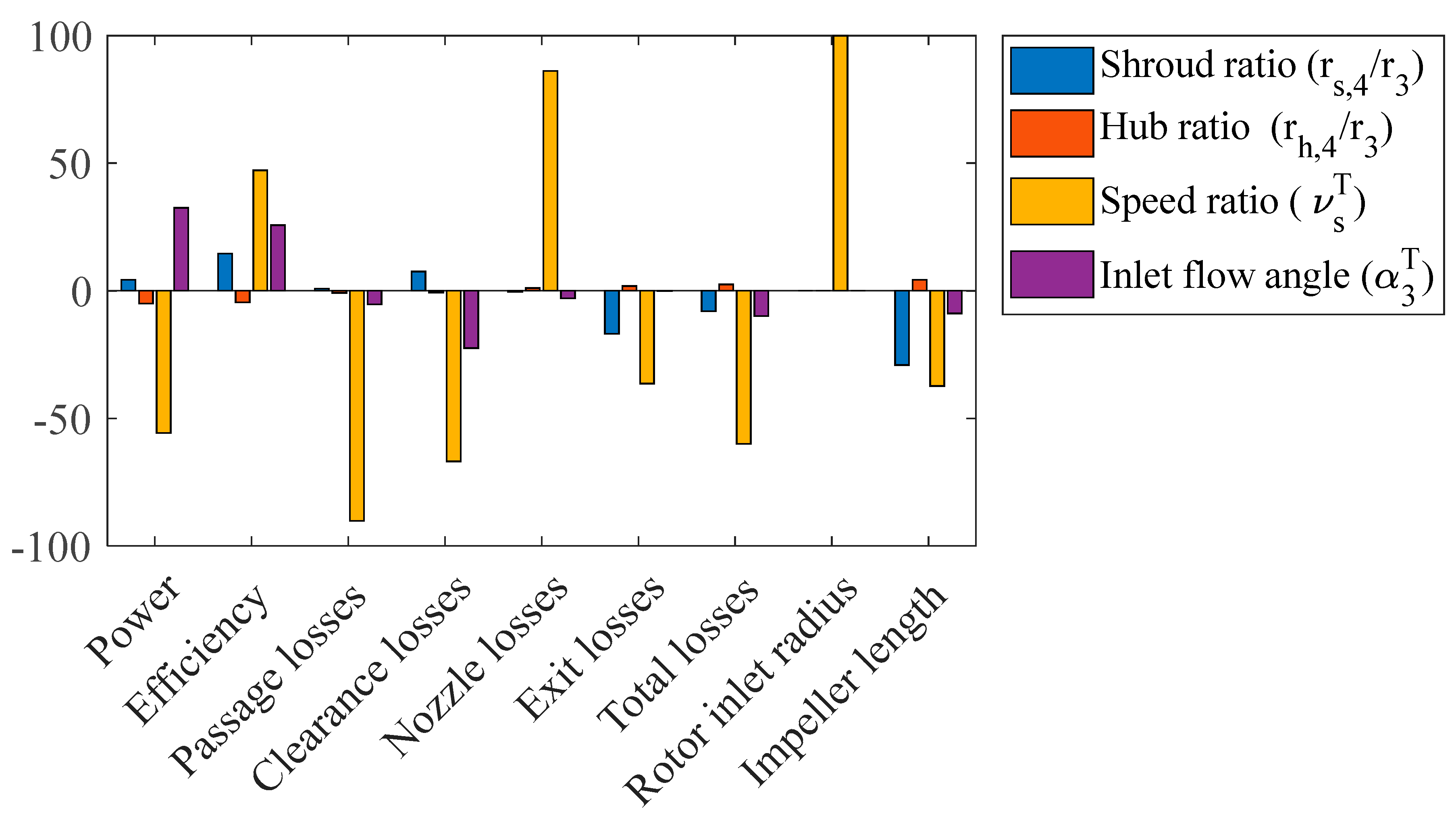
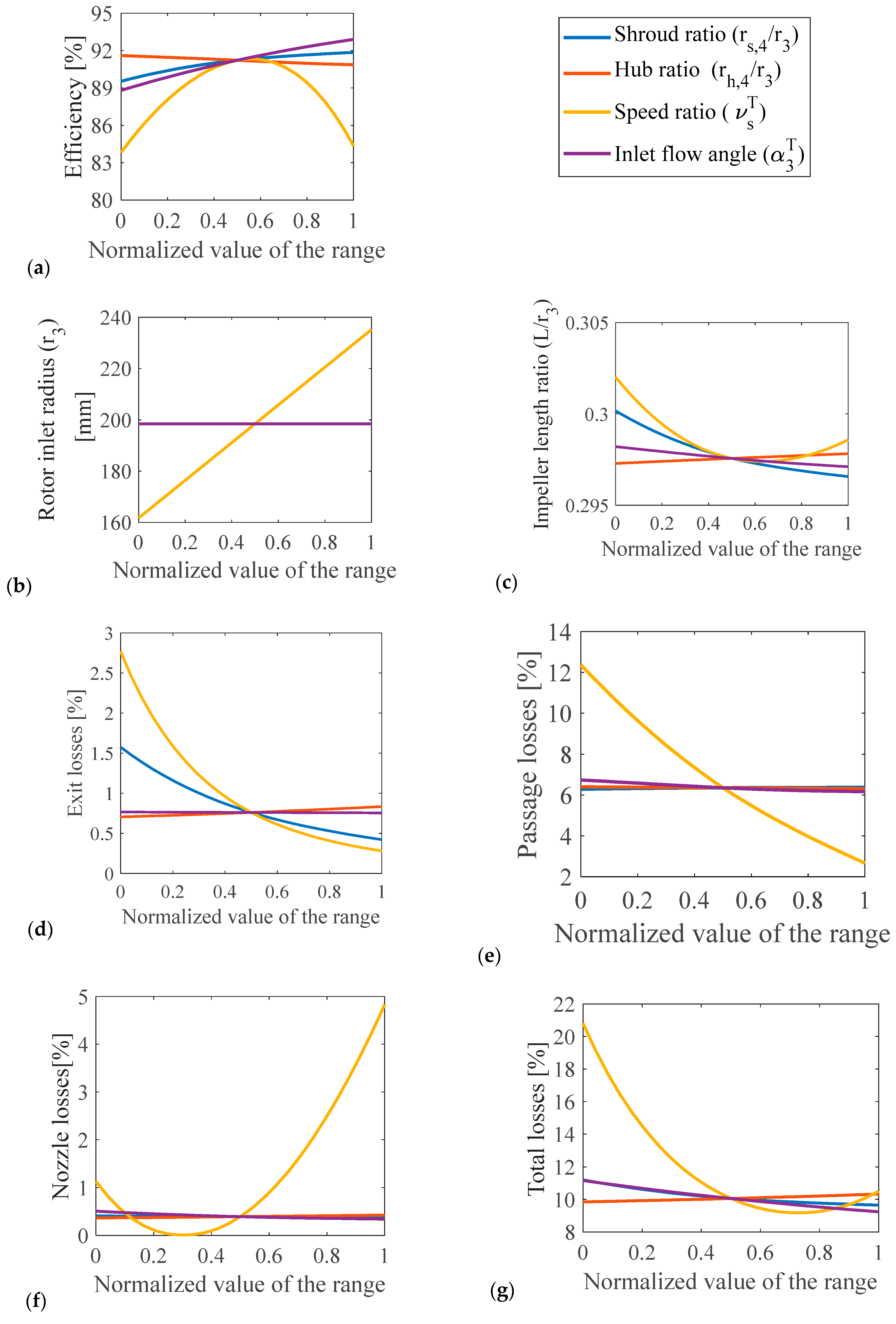
• It is noted that the turbine’s performance parameters (power, efficiency, various types of losses, rotor radius, and impellor length) are most sensitive to the speed ratio (${\nu }_s$) followed by the inlet flow angle (${\alpha }_3$). At the same time, the turbine’s performance is observed to be least sensitive to the turbine’s hub ratio.
• It is found that the rotor’s efficiency changes considerably by changing the design parameters, i.e., shroud ratio ($\frac{r_{s4}}{r_3})$ hub ratio ($\frac{r_{s4}}{r_3})$, speed ratio $\left({\nu }_s\right)$ and inlet flow angle $\left({\alpha }_3\right)$. Conversely, the rotor’s size is only affected by the speed ratio $\left({\nu }_s\right),$ i.e., rotor inlet radius $r_3$, which rises considerably by increasing the value of the speed ratio, although, shroud ratio ($\frac{r_{s4}}{r_3})$ hub ratio ($\frac{r_{s4}}{r_3})$ and inlet flow angle $\left({\alpha }_3\right)$ do not impart any significant impact on the rotor’s size.
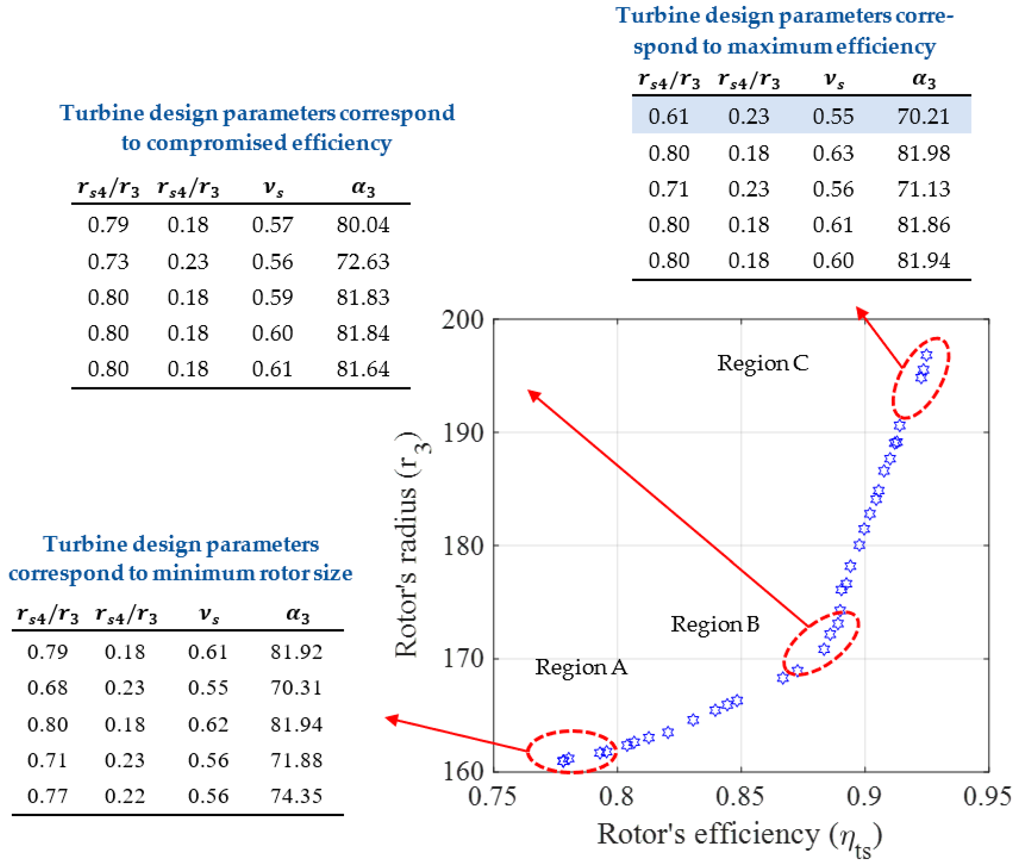
• Optimization results suggest that the dependence of design input parameters on the performance and sizing of the turbine is quite complex, and it is difficult to conclude the effect of individual parameters without contemplating their combined effect. Therefore, the design and analysis of the turbine would require multifaceted techniques such as the one used in the current study to understand the absolute behavior of any individual turbine design parameter.
• It is found that the turbine’s minimum size corresponds to the design with the lowest efficiency; however, the turbine’s efficiency can be improved at the cost of the increased size of the turbine’s rotor. Heat exchangers are the largest components in the sCO₂-BC [4] and take up most of its layout space; therefore, design of the turbine with higher efficiency is recommended, despite the fact that it will increase the size of the turbine, as it will not impact the overall layout size of the sCO₂-BC.
• Analysis of a range of design variables consumes a huge amount of computational time and resources. Therefore, by combining computational fluid dynamics with machine learning algorithms, efficient and cost-effective methods for design optimization can be achieved. In this study, the computational cost is reduced substantially by utilizing trained DNN and MOGA optimization processes, and this DNN-MOGA methodology can be extended to other applications of design optimization. However, it is to be noted here that data used for the training in this work is limited to an 8-Megawatt turbine system for sCO₂-BC and cannot be used for expander systems with different power outputs.

References

- UNFCCC. The Paris Agreement. Available online: http://unfccc.int/paris_agreement/items/9485.php (accessed on 16 October 2021).
- World Energy Council. World Energy Resources, 2016. Available online: https://www.worldenergy.org/wp-content/uploads/2016/10/World-Energy-Resources-Full-report-2016.10.03.pdf (accessed on 16 October 2021).
- Fundamentals and Applications of Supercritical Carbon Dioxide (sCO2) Based Power Cycles; Brun, K.; Friedman, P.; Dennis, R. (Eds.) Woodhead Publishing: Sawston, Cambridge, MA, UK, 2017. [Google Scholar]
- Saeed, M.; Awais, A.A.; Berrouk, A.S. CFD aided design and analysis of a precooler with zigzag channels for supercritical CO2 power cycle. Energy Convers. Manag. 2021, 236, 114029. [Google Scholar] [CrossRef]
- Saeed, M.; Khatoon, S.; Kim, M.-H. Design optimization and performance analysis of a supercritical carbon dioxide recompression Brayton cycle based on the detailed models of the cycle components. Energy Convers. Manag. 2019, 196, 242–260. [Google Scholar] [CrossRef]
- Sienicki, J.; Moisseytsev, A.; Fuller, R.L.; Wright, S.A.; Pickard, P.S. Scale dependencies of supercritical carbon dioxide brayton cycle technologies and the optimal size for a next-Step supercritical CO2 cycle demonstration. In Proceedings of the sCO2 Power Cycle Symposium, Boulder, CO, USA, 24–25 May 2011. [Google Scholar]
- Dostal, V.; Michael, J.D.; Hejzlar, P. A Supercritical Carbon Dioxide Cycle for Next Generation Nuclear Reactors, MIT-ANP-TR-100, Advanced Nuclear Power Technology Program Report. Ph.D. Thesis, Massachusetts Institute of Technology, Cambridge, MA, USA, 2004. [Google Scholar]
- Zhang, H.; Zhao, H.; Deng, Q.; Feng, Z. Aerothermodynamic design and numerical investigation of supercritical carbon dioxide turbine. In Proceedings of the ASME Turbo Expo, Montréal, QC, Canada, 15–19 June 2015. [Google Scholar]
- Odabaee, M.; Sauret, E.; Hooman, K. CFD simulation of a supercritical carbon dioxide radial-inflow turbine, comparing the results of using real gas equation of estate and real gas property file. Appl. Mech. Mater. 2016, 846, 85–90. [Google Scholar] [CrossRef]
- Luo, D.; Liu, Y.; Sun, X.; Huang, D. The design and analysis of supercritical carbon dioxide centrifugal turbine. Appl. Therm. Eng. 2017, 127, 527–535. [Google Scholar] [CrossRef]
- Kalra, C.; Sevincer, E.; Brun, K.; Hofer, D.; Moore, J. Development of high efficiency hot gas turbo-expander for optimized CSP supercritical CO2 power block operation. In Proceedings of the 4th International Symposium Supercritical CO2 Power Cycles, Pittsburgh, PA, USA, 9–10 September 2014. [Google Scholar]
- Lindqvist, K.; Wilson, Z.T.; Næss, E.; Sahinidis, N.V. A machine learning approach to correlation development applied to fin-tube bundle heat exchangers. Energies 2018, 11, 3450. [Google Scholar] [CrossRef] [Green Version]
- Song, J.; Tian, W.; Xu, X.; Wang, Y.; Li, Z. Thermal performance of a novel ultrasonic evaporator based on machine learning algorithms. Appl. Therm. Eng. 2019, 148, 438–446. [Google Scholar] [CrossRef]
- Longo, G.A.; Mancin, S.; Righetti, G.; Zilio, C.; Ortombina, L.; Zigliotto, M. Application of an Artificial Neural Network (ANN) for predicting low-GWP refrigerant boiling heat transfer inside Brazed Plate Heat Exchangers (BPHE). Int. J. Heat Mass Transf. 2020, 160, 119824. [Google Scholar] [CrossRef]
- Zhao, X.; Shirvan, K.; Salko, R.K.; Guo, F. On the prediction of critical heat flux using a physics-informed machine learning-aided framework. Appl. Therm. Eng. 2020, 164, 114540. [Google Scholar] [CrossRef]
- Zhang, A. Machine Learning-Based Design Optimization of Centrifugal Impellers. In The Global Power and Propulsion Society; 2021. [Google Scholar]
- Omidi, M.; Liu, S.J.; Mohtaram, S.; Lu, H.T.; Zhang, H.C. Improving centrifugal compressor performance by optimizing the design of impellers using genetic algorithm and computational fluid dynamics methods. Sustainability 2019, 11, 5409. [Google Scholar] [CrossRef] [Green Version]
- Shi, D.; Sun, L.; Xie, Y. Off-design performance prediction of a S-CO2 turbine based on field reconstruction using deep-learning approach. Appl. Sci. 2020, 10, 4999. [Google Scholar] [CrossRef]
- Ilmini, K.; Fernando, T. Persons’ Personality Traits Recognition using Machine Learning Algorithms and Image Processing Techniques. Adv. Comput. Sci. Int. J. 2016, 5, 40–44. [Google Scholar]
- Saeed, M.; Kim, M. Analysis of a recompression supercritical carbon dioxide power cycle with an integrated turbine design/optimization algorithm. Energy 2018, 165, 93–111. [Google Scholar] [CrossRef]
- Massimiani, A.; Palagi, L.; Sciubba, E.; Tocci, L. Neural networks for small scale ORC optimization. Energy Procedia 2017, 129, 34–41. [Google Scholar] [CrossRef]
- Villarrubia, G.; de Paz, J.F.; Chamoso, P.; De la Prieta, F. Artificial neural networks used in optimization problems. Neurocomputing 2018, 272, 10–16. [Google Scholar] [CrossRef]
- Aungier, A.H. Turbine Aerodynamics: Axial-Flow and Radial-Flow Turbine Design and Analysis; ASME: New York, NY, USA, 2006; pp. 10016–15990. [Google Scholar]
- Moustapha, H. Axial and Radial Turbines, 1st ed.; Concepts NREC: VT, USA, 2003; Available online: https://www.researchgate.net/publication/238778854_Axial_and_Radial_Turbines (accessed on 16 October 2021).
- Fouad, W.A.; Berrouk, A.S. Prediction of H2S and CO2 Solubilities in Aqueous Triethanolamine Solutions Using a Simple Model of Kent-Eisenberg Type. Ind. Eng. Chem. Res. 2012, 51, 6591–6597. [Google Scholar] [CrossRef]
- Althuluth, M.; Berrouk, A.S.; Kroon, M.C.; Peters, C.J. Modeling solubilities of gases in the ionic liquid 1-ethyl-3-methylimidazolium tris (pentafluoroethyl) trifluorophosphate using the Peng–Robinson equation of state. Ind. Eng. Chem. Res. 2014, 53, 11818–11821. [Google Scholar] [CrossRef]
- Lemmon, E.; Linden, M.M.; Huber, M. NIST Reference Fluid Thermodynamic and Transport Properties Database: REFPROP Version 9.1, NIST Standard Reference Database 23, 2013., n.d. Available online: http://www.boulder.nist.gov (accessed on 25 December 2017).
- Watanabe, I.; Ariga, I.; Mashimo, T. Effect of Dimensional Parameters of Impellers on Performance Characteristics of a Radial-Inflow Turbine. J. Eng. Power 1971, 93, 81–102. [Google Scholar] [CrossRef]
- Saeed, M.; Alawadi, K.; Kim, S.C. Performance of Supercritical CO2 Power Cycle and Its Turbomachinery with the Printed Circuit Heat Exchanger with Straight and Zigzag Channels. Energies 2021, 14, 62. [Google Scholar] [CrossRef]
- Saeed, M.; Berrouk, A.S.; Siddiqui, M.S.; Awais, A.A. Effect of Printed Circuit Heat Exchanger’s Different Designs on the Performance of Supercritical Carbon Dioxide Brayton Cycle. Appl. Therm. Eng. 2020, 179, 115758. [Google Scholar] [CrossRef]
- Saeed, M.; Berrouk, A.S.; AlShehhi, M.S.; AlWahedi, Y.F. Numerical investigation of the thermohydraulic characteristics of microchannel heat sinks using supercritical CO2 as a coolant. J. Supercrit. Fluids 2021, 176, 105306. [Google Scholar] [CrossRef]
- Abadi, M.; Agarwal, A.; Barham, P.; Brevdo, E.; Chen, Z.; Citro, C.; Corrado, G.S.; Davis, A.; Dean, J.; Devin, M.; et al. TensorFlow: Large-Scale Machine Learning on Heterogeneous Distributed Systems. In Proceedings of the 12th USENIX Symposium on Operating Systems Design and Implementation, Savannah, GA, USA, 2–4 November 2016. [Google Scholar]
- Saeed, M.; Radaideh, M.I.; Berrouk, A.S.; Alawadhi, K. Machine Learning-based Efficient Multi-layered Precooler Design Approach for Supercritical CO2 Cycle. Energy Convers. Manag. X 2021, 11, 100104. [Google Scholar] [CrossRef]
- Rebai, N.; Hadjadj, A.; Benmounah, A.; Berrouk, A.S.; Boualleg, S.M. Prediction of Natural Gas Hydrates Formation Using a Combination of Thermodynamic and Neural Network Modelling. J. Petrol. Sci. Eng. 2019, 182, 10627. [Google Scholar] [CrossRef]
- Chu, Y.M.; Ibrahim, M.; Saeed, T.; Berrouk, A.S.; Algehyne, E.A.; Kalbasi, R. Examining Rheological Behavior of MWCNT-TiO2/5W40 Hybrid Nanofluid Based on Experiment and RSM/ANN Modeling. J. Mol. Liq. 2021, 333, 115969. [Google Scholar] [CrossRef]
- Goldberg, D.E.; Samtani, M.P. Engineering Optimization via Genetic Algorithm. In Electronic Computation; ASCE: Reston, VA, USA; Washington, DC, USA, 1986; pp. 471–482. Available online: https://www.researchgate.net/publication/246069860_Engineering_optimization_via_genetic_algorithm (accessed on 16 October 2021).
- Siddiqui, M.S.; Latif, S.T.M.; Saeed, M.; Rahman, M.; Badar, A.W.; Hasan, S.M. Reduced order model of offshore wind turbine wake by proper orthogonal decomposition. Int. J. Heat Fluid Flow 2020, 82, 108554. [Google Scholar] [CrossRef]
- Siddiqui, M.S.; Hamza, M.; Waheed, A.; Saeed, M. Parametric Analysis Using CFD to Study Impact of Geometric and Numerical Modeling on the Performance of Small-Scale Horizontal Axis Wind Turbine, (n.d.). Available online: https://www.mdpi.com/1996-1073/13/15/3880/htm (accessed on 16 October 2021).
- Saeed, M.; Berrouk, A.S.; Siddiqui, M.S.; Awais, A.A. Numerical investigation of thermal and hydraulic characteristics of sCO2-water printed circuit heat exchangers with zigzag channels. Energy Convers. Manag. 2020, 224, 113375. [Google Scholar] [CrossRef]
- Saeed, M.; Berrouk, A.S.; Singh, M.P.; Alawadhi, K. Analysis of Supercritical CO2 Cycle Using Zigzag Channel Pre-Cooler: A Design Optimization Study Based on Deep. Energies 2021, 14, 6227. [Google Scholar] [CrossRef]