Modeling and Monitoring Erosion of the Leading Edge of Wind Turbine Blades

Abstract

Leading edge surface erosion is an emerging issue in wind turbine blade reliability, causing a reduction in power performance, aerodynamic loads imbalance, increased noise emission, and, ultimately, additional maintenance costs, and, if left untreated, it leads to the compromise of the functionality of the blade. In this work, we first propose an empirical spatio-temporal stochastic model for simulating leading edge erosion, to be used in conjunction with aeroelastic simulations, and subsequently present a deep learning model to be trained on simulated data, which aims to monitor leading edge erosion by detecting and classifying the degradation severity. This could help wind farm operators to reduce maintenance costs by planning cleaning and repair activities more efficiently. The main ingredients of the model include a damage process that progresses at random times, across multiple discrete states characterized by a non-homogeneous compound Poisson process, which is used to describe the random and time-dependent degradation of the blade surface, thus implicitly affecting its aerodynamic properties. The model allows for one, or more, zones along the span of the blades to be independently affected by erosion. The proposed model accounts for uncertainties in the local airfoil aerodynamics via parameterization of the lift and drag coefficients’ curves. The proposed model was used to generate a stochastic ensemble of degrading airfoil aerodynamic polars, for use in forward aero-servo-elastic simulations, where we computed the effect of leading edge erosion degradation on the dynamic response of a wind turbine under varying turbulent input inflow conditions. The dynamic response was chosen as a defining output as this relates to the output variable that is most commonly monitored under a structural health monitoring (SHM) regime. In this context, we further proposed an approach for spatio-temporal dependent diagnostics of leading erosion, namely, a deep learning attention-based Transformer, which we modified for classification tasks on slow degradation processes with long sequence multivariate time-series as inputs. We performed multiple sets of numerical experiments, aiming to evaluate the Transformer for diagnostics and assess its limitations. The results revealed Transformers as a potent method for diagnosis of such degradation processes. The attention-based mechanism allows the network to focus on different features at different time intervals for better prediction accuracy, especially for long time-series sequences representing a slow degradation process.

1. Introduction

This work was motivated by current efforts on development of a novel micro-electro-mechanical monitoring system based on aerodynamic surface pressure and aero-acoustic measurements for structural health monitoring of wind turbine blades, as part of the Aerosense project [1]. Sensing nodes are distributed along the span of the blade, delivering measurements of local sectional aerodynamic pressure distributions and aero-acoustic and acceleration signals (see the illustration in Figure 1). Assuming the availability of such a monitoring system, we proposed an approach to the modeling and diagnostics of erosion of the leading edge for wind turbine blades.

Leading-edge erosion (LEE) is caused by environmental variations in the blade surface, temperature oscillations, moisture, UV radiation, raindrops, sand, and hailstones or other particles impacting the leading edge of the blade. It could also be initiated by surface cracks due to global strain from blade flexing [2], errors during manufacturing in terms of paint deposits, consistency of the gel coat thickness and bonding strength, or initiating surface damage during blade handling in transport or installation. This causes the surface material to be removed from the blade surface, leaving a rough profile that degrades the aerodynamic performance, and, in the long term, if left untreated, it impacts the structural integrity of the blade. Outboard blade regions, where the relative velocity of the flow is higher, may exhibit more prominent erosion levels as impacts with eroding elements are more energetic. Moreover, the outboard sectional regions have a more significant role in power production, which further exacerbates rotor performance degradation.

Bogdanoff and Kozin (1985) [3] define cumulative damage as the “irreversible accumulation of damage throughout life that ultimately leads to failure.” Leading edge erosion of a wind turbine blade represents such a process, albeit at slow degradation rates, with effects slow to manifest and even harder to detect early on. Most diagnostic techniques today rely on direct visual inspection [4], image processing [5], and statistical analysis, e.g., regression or clustering of supervisory control and data acquisition (SCADA) output, such as blade pitch, rotor speed, or electrical power [6,7]. Visual inspection and image acquisition generally imply occasional stoppage of the turbines, resulting in loss of power production. More importantly, they give a local (both spatial and temporal) snapshot of the erosion condition without a direct link to the historical progression of the degradation and how it relates to environmental and operational conditions. Even though it is better positioned to discriminate the environmental and operational conditions versus the degradation process, long-term SCADA-based statistical analysis invariably does not possess the necessary resolution to determine accurately the severity and spatial extent of erosion on the blades. A gap therefore exists in the field of spatio-temporal modeling and diagnostics of leading edge erosion for wind turbines rotor blades. In this work, we were particularly interested in leveraging time series emanating from the novel Aerosense-based aerodynamic surface pressure monitoring system for wind turbines’ blades. The aim was to (1) detect the occurrence of erosion and (2) classify the severity (intensity) of erosion. This could be regarded as either the inverse problem of reconstruction for the lift and drag coefficients or a problem of finding the optimal discriminants for erosion versus other effects from time-series response signals. To tackle this problem and build meaningful diagnostics models, realistic time-series data were required for training. Our options were either to collect multi-year field data, where the rotor blades are known to undergo leading edge erosion, or to develop a numerical model of erosion coupled to an aeroelastic simulator. As data availability for such systems is often limited and restricted by data-sharing protocols, we here opted for the route of numerical modeling and simulations, with the additional benefit of delivering a model that can be used for simulating such slow leading edge erosion degradation processes.

Towards accomplishing the goal of diagnostics and inference of erosion of the leading edge of wind turbine blades, this work made the following contributions:

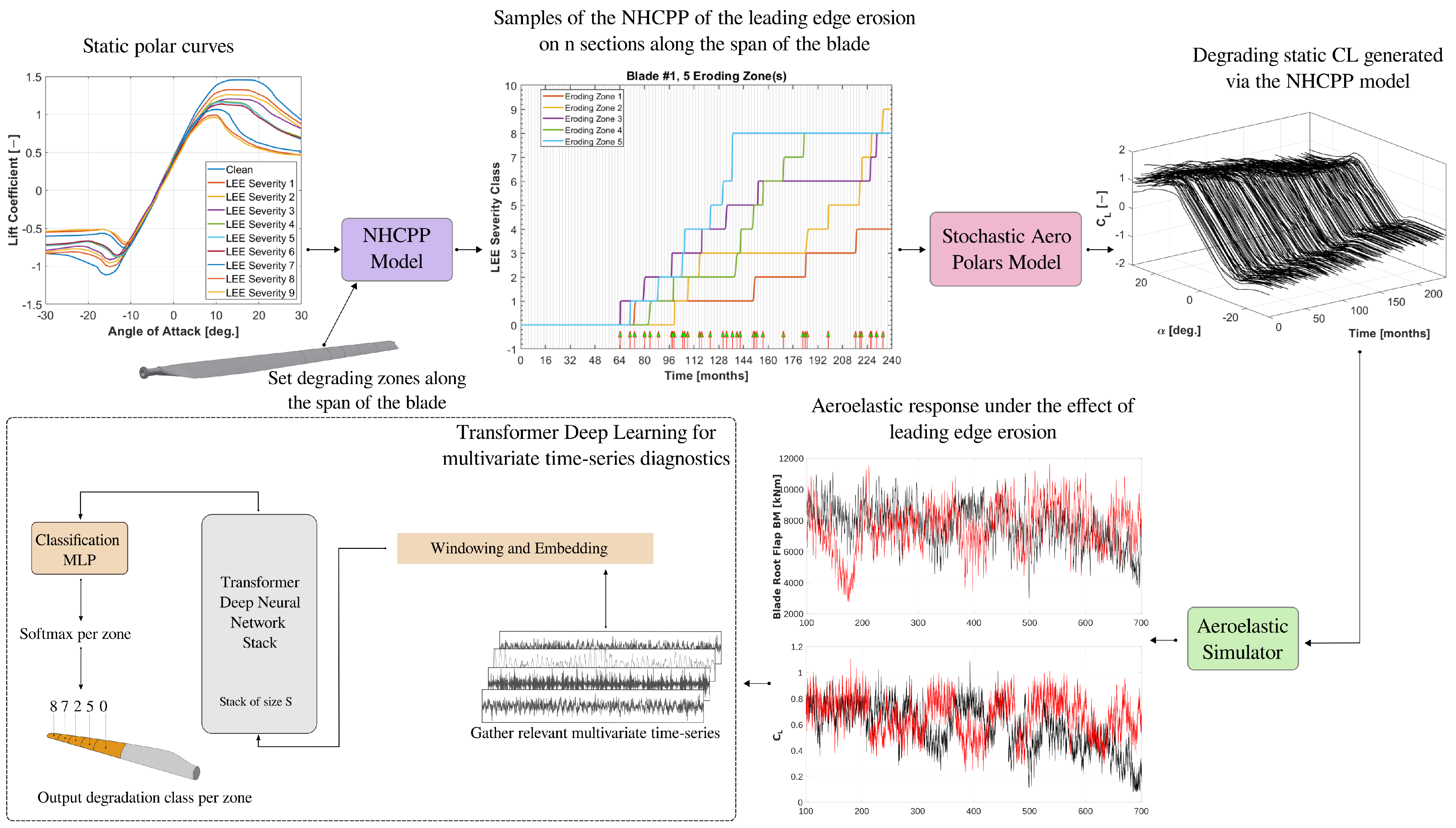
• We developed a stochastic spatio-temporal erosion model of the leading edge of wind turbine blades, which is characterized by a non-homogeneous compound Poisson process across discrete states, embedded in a generator of a stochastic ensemble of degrading airfoil aerodynamic polars for use in forward aero-servo-elastic simulations. The coupled model is able to compute the aeroelastic non-stationary response of a wind turbine, thus reflecting its behavior under the effect of leading edge erosion and varying turbulent input inflow conditions over a long period of degradation.
• We adapted a deep-learning multivariate time-series-based Transformer, which employs attention mechanisms to detect and classify long-term and slow leading edge erosion processes assuming the availability of on-blade sectional monitoring data, under short- and long-term wind inflow uncertainties and aerodynamic uncertainties on the lift and drag coefficients of the airfoil sections along the span of the blade.

A graphical abstract of this research is presented in Figure 2.

The remainder of this article is organized as follows. In Section 2, we offer a review of the state of the art in the modeling and diagnostics of leading-edge erosion. In Section 3, we present the details of the spatio-temporal stochastic model for leading-edge erosion. In Section 4, we present the uncertainty modeling and the aeroelastic simulations setup. In Section 5, we elaborate the theory of the Transformer model for diagnostics and inference. In Section 6, we illustrate the novelty and principles of the proposed framework on a simulations-based application and further provide discussions and list the limitations in Section 7.

2. Review of Prior Art

We review modeling approaches of leading edge erosion in conjunction with aeroelastic simulations and subsequently assess the state-of-the-art in diagnostics methods.

2.1. Modelling Leading-Edge Erosion

Several studies have quantified the impact of leading-edge erosion on the aerodynamic and aeroelastic performance of wind turbines.

The general thread in the first set of studies amounts to describing the constitutive laws, physical processes, and instigators at the micro-scale resulting in surface erosion/degradation and the various stages and types of erosion severity e.g., [2,8,9,10,11]. Such models incorporate the effect of wind speed, air density, particle size, incubation time, and erosion intensity due to rainfall, snowfall, sea spray, and fog. It is unclear however how the micro-scale models couple to the macro-scale aspects of leading-edge erosion and consequently the effect on turbine performance.

The second set of studies quantified the impact on wind turbine performance via computational approaches (aeroelastic or computational fluid dynamics simulations) or extensive experimental campaigns in wind tunnels, coupled to uncertainty propagation schemes e.g., [12,13,14,15,16,17]. The limitations in all these works is that they do not allow for multiple zones along the span of the blades to be independently affected by stochastic erosion processes.

Bortolotti et al. [18] proposed a simple stochastic model to describe the extent of blade span-wise degradation due to leading-edge erosion via a single factor that was assumed to follow a truncated beta distribution. However, the long-term temporal degradation process of the blade’s leading-edge was not accounted for. Dimitrov [19] describes a first attempt to introduce temporal progression to the damage growth for leading-edge erosion due to rainfall events indirectly via loss of annual energy production.

To the best of our knowledge, we found a gap in the existing literature for comprehensive models that encompass both stochastic, spatial, and temporal elements to describe the erosion process of the leading edge of wind turbine blades and the effects on their performance over long periods of degradation time horizons.

2.2. Diagnosing Leading Edge Erosion

Different approaches exist to diagnose the extent of leading-edge erosion on wind turbine blades. Traditionally, manual human inspection was used, although modern visual approaches are being developed to utilize drones paired with computer vision [5]. Our aim was to use data-driven continuous monitoring methods to perform diagnostics without resorting to turbine shutdown. We review different machine learning and probabilistic approaches that have been put forth and which, given data recorded by sensors placed on the wind turbine (e.g., novel aerodynamic pressure sensors, SCADA, accelerometers, strain gauges, etc.), would be able to estimate the extent of leading-edge erosion on wind turbine blades. In this context, the diagnostics task can be described as a multivariate time-series (MTS) classification/clustering problem; an algorithm is tasked with predicting the degradation status/class of a blade by analyzing multiple time-dependent signals. We therefore included MTS methods, which have not been specifically applied to wind turbine blades in the past, allowing us to explore promising machine learning approaches from diverse fields unrelated to structural health monitoring: activity recognition, anomaly detection, sound analysis, human health signal (EEG and ECG), interpretation, etc. If the forward model of the degradation process is known, the diagnostics problem becomes a supervised classification task, seeing that each MTS data point is associated with its degradation ground truth. Data-driven MTS classification is a field that is currently generating a significant amount of attention, with many promising methods that have been recently developed [20]. Within these approaches, we can differentiate between those that use the raw time-series data [21], known as end-to-end approaches, and those that first extract features that are then passed to a classification algorithm [22].

Extracting features from time-series data can be accomplished in many ways, with domain-dependent feature engineering or statistical methods often being the first choices. Algorithms based on empirical mode decomposition (EMD) are implemented for representing MTS as a superposition of simpler well-behaved components called intrinsic mode functions (IMFs). EMD approaches are suitable for damage detection and degradation state recognition in the analysis of nonlinear and non-stationary signals. However, they have shown low performance in highly stochastic signals with spike pulses and jumps [23,24]. Distance-based metrics evaluate the similarity between time-series data form another popular class of conventional feature construction methods [25]. Alternatively, in [26,27], feature vectors are built from MTS data by passing the inputs through numerous random convolutional kernels. This approach, named ROCKET, has a relatively low computational cost, yet, when combined with a standard ridge classifier, it achieves state-of-the-art accuracy on the UCR time-series archive dataset [28]. Other methods turn the time-series inputs into feature images [29], which are then fed into convolutional neural networks (CNNs) [30] designed for image classification, thus taking advantage of the recent advances in computer vision performance. Although feature engineering and feature extraction can potentially lead to accurate diagnostics with good explainability, we were interested in implementing end-to-end methods that use raw MTS data. This is due to the fact that feature-based methods often require large amounts of cumbersome human intervention, which limits generalization. Robustness is another potential downside, where changing the input, due to sensor malfunction for instance, might require re-selecting relevant features, while it can be factored into end-to-end approaches, provided it is part of the training data.

Conventional (“shallow”) data-driven classification methods do not often use untransformed MTS as inputs, due to the difficulty associated with extracting relevant information from noisy, complex data. In contrast, deep-learning methods often excel at learning hidden discriminative features, making them particularly well suited for end-to-end approaches [31]. CNNs have been applied to end-to-end MTS classification in the context of prognostic health management [32], surgeon skill classification [33], and other tasks [34]. CNNs are limited by their receptive field, making their use limited to relatively short time-series. Recurrent neural networks (RNNs) [35] are, by design, effective at solving tasks relating to sequential data. Long short-term memory (LSTM) networks [36], currently the most commonly used type of RNNs, have been used to successfully classify clinical measurements [37] and action recognition tasks [38]. However, RNNs are also limited to relatively short input sequences due to memory requirements and are difficult to train. In recent years, Transformers [39] have attracted a lot of attention in the Natural Language Processing (NLP) community and have mostly replaced RNNs. These neural networks leverage the power of attention mechanisms to learn the relevant interdependencies within sequences. Transformers have increasingly been applied in other domains, such as computer vision [40], time-series forecasting [41], and multivariate time-series classification [42]. Graph neural networks [43], a class of deep data-driven methods that utilize graph-structured data, have also been applied to end-to-end MTS classification [44]. This is done by first constructing an adjacency matrix from the untransformed MTS data. In [45], spatio-temporal graph Transformer neural networks (GTNN) were implemented in order to effectively capture both dynamic spatial and temporal trends. We could envisage using a GTNN model to leverage temporal and spatial correlations in the degrading sections of the three blades on a wind turbine.

As previously mentioned, deep end-to-end models are, in general, better suited for generalization than feature-extraction approaches. Moreover, they can be further optimized for transferability [46], for instance by applying transfer learning methods, such as using domain adaption layers [47].

In the context of data-driven wind turbine blade condition monitoring, a number of methods have been reported in the literature [48]. In [49] vibrational, frequency response functions were used as input features to neural networks, in order to detect changes in the structural health of a blade. LSTMs were trained to classify faults, based on multivariate sensor recordings of a model wind turbine test rig in [50], while [51] implemented a CNN to detect possible wind turbine blade breakages based on SCADA data. In [52], support vector machines were trained on features built from active acoustic recordings to diagnose healthy and damaged states of a model wind turbine. Another feature-extraction approach was combined with decision trees in [53] to diagnose different fault scenarios for a model wind turbine. Finally, ice buildup on wind turbine blades was predicted with random forests trained on SCADA data in [54], while Weijtjens et al. [55] used Gaussian processes trained on data emanating from low-cost tower-mounted sensors to do so.

Considering their extensive use in other domains, Transformers bear great potential for SHM damage detection. Some researchers have made use of attention mechanisms similar to those found in Transformers for bearing remaining useful life prediction [56], but to the best of the authors’ knowledge, only in [57] have proper Transformer models been used in this context. In this work, however, an end-to-end approach was not used; instead, the model was fed a pre-processed input composed of time series features such as Mel frequency Cepstral coefficients (MFCCs) and short-time Fourier transformation (STFT). We chose Transformers as the base of our end-to-end approach for diagnostics. However, we implemented additional modifications so as to be able to handle multivariate sequences on the order of several 10s of thousands of data points while still being able to track long-term degradation progression, reflected by newly sampled sequences with possible discontinuities. Few, if any, of the existing MTS learning models discussed above are capable of this.

3. Modeling Erosion of the Leading Edge

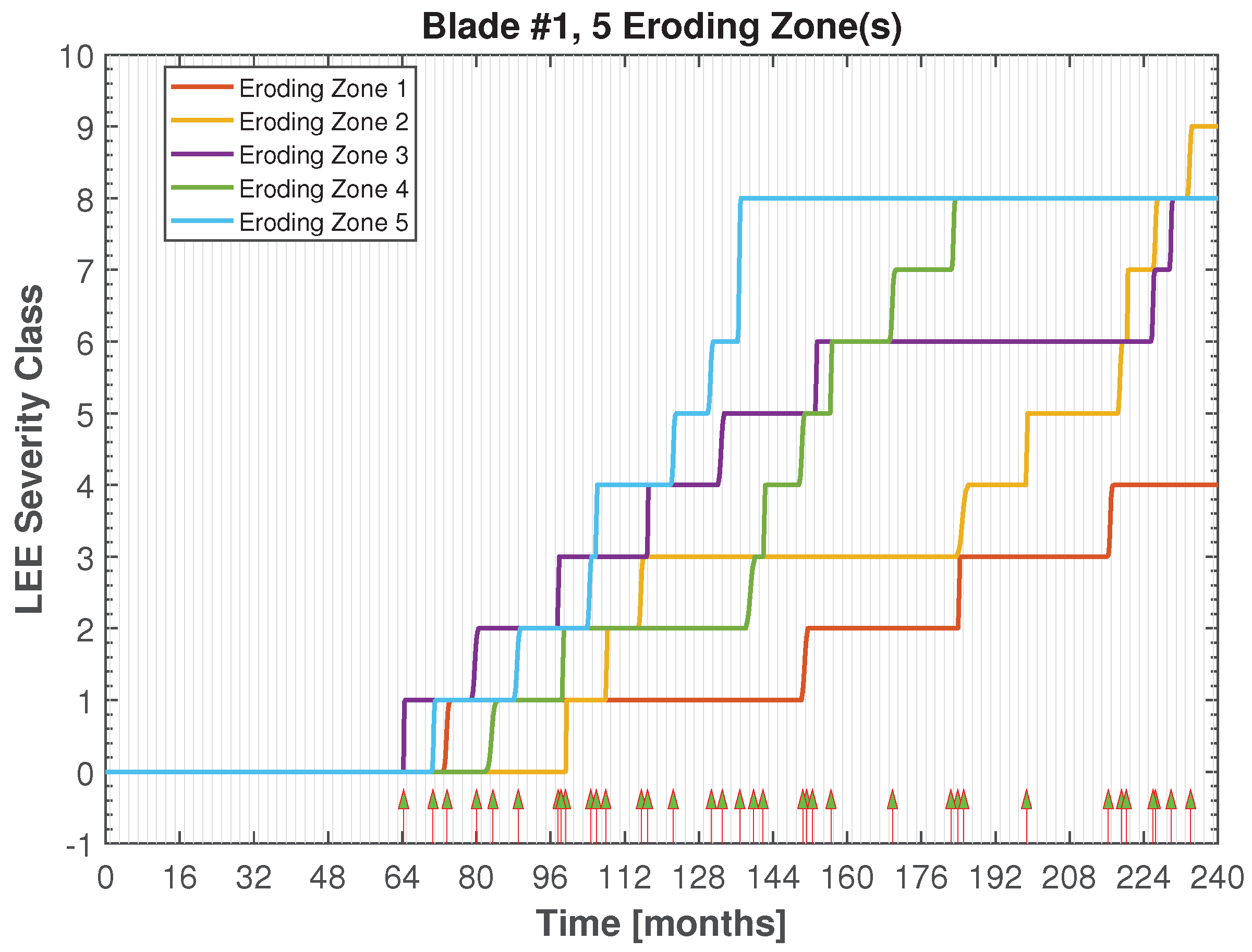
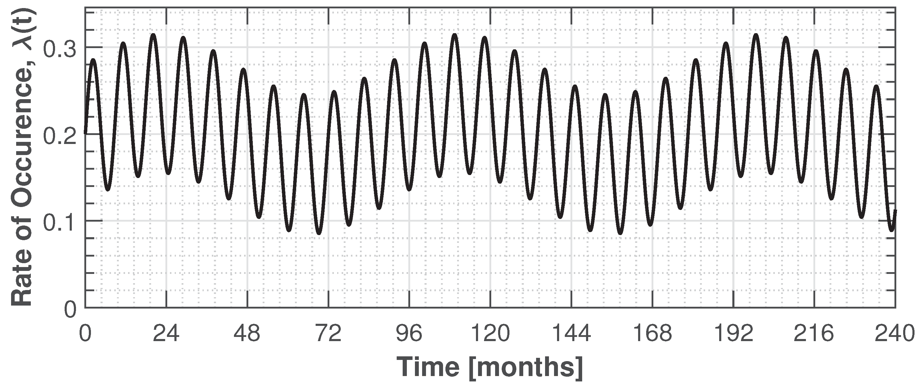
3.1. Non-Homogeneous Compound Poisson Process

Erosion initiates on the blades in the form of pits near the leading edge on the pressure side. These pits develop gradually over time into gouges, then steadily grow in their size and density to coalesce as delaminations. Gaudern [9] identified five categories of erosion severity classes. In Sareen et al. [8], we find an analysis of the effect of erosion at the leading edge on the aerodynamic performance of the $DU96-W-180$ airfoil and categorized erosion from pits to delamination in different types and stages (9 in total), as shown in

Table 1. Types and stages of leading-edge erosion with the number of pits (P), number of gouges (G), and magnitude of leading edge delamination (DL), modified from [8].

	Stage 1	Stage 2	Stage 3	Stage 4	Stage 5
Type A	100P	200P	400P	—	—
Type B	—	200P/100G	400P/200G	800P/400G	—
Type C	—	—	400P/200G/DL	800P/400G/DL+	1600P/800G/DL++

. Each combination of type and stage of erosion has associated with it aerodynamic polar curves ($C_L$, $C_D$, $C_M$) derived via measurements in a wind tunnel [8,9,12]. Throughout the article we adopt a similar labeling of the leading-edge erosion severity as shown in

Table 2. Class labels adopted for the severity categorization of leading edge erosion.

	Stage 1	Stage 2	Stage 3	Stage 4	Stage 5
Type A	1	2	3	—	—
Type B	—	4	5	6	—
Type C	—	—	7	8	9

.

We proposed a two-step empirical spatio-temporal stochastic model of LEE. Step 1 of the model includes a damage process that occurs at random times, emulating the non-stationary time of arrival of degradation and its magnitude, with 10 discrete states based on the non-homogeneous compound Poisson process (NHCPP) to describe the random degradation of the blade surface and implicitly its aerodynamic properties. In step 2 of the model, the local leading edge degradation manifests by physical changes in the aerodynamic polars. This step generates an ensemble of stochastic aerodynamic polars for a given erosion severity of LEE in NHCPP by parameterizing the lift and drag coefficients curves [58].

A non-homogeneous Poisson process (NHPP) is a stochastic degradation process over a finite time horizon. The NHPP $\{N\left(t\right),t\ge 0\}$ has rate of arrivals $\lambda \left(t\right)$ on the time interval $t\in \left[0,T\right]$. A sample path of a NHCPP emulates two main properties in the proposed LEE: (1) random time of arrival, $0\le {\tau }_1\le {\tau }_2\le \cdots$: these are the time instances corresponding to a change in the degradation level of an airfoil’s aerodynamic properties (shocks) and (2) the magnitude of change $\{Y_n,n\ge 1\}$ in the degradation level of an airfoil aerodynamic properties at the nth time of arrival. In practice, for a probabilistic assessment, many NHPP paths are sampled. The model incorporates one or more zones (adjacent or disjoint) along the span of the blade(s) affected by erosion, but they are assumed to undergo independent degradation processes. The NHCPP modifies the definition of a Poisson process so that it can incorporate a time-dependent rate. The NHPP is suitable given the fact that the rate of LEE is not constant in time; on the short time scales (hourly), it is dependent on the rotor speed due to variations in the wind speed, while, on the longer time scales, it is dependent on seasonal variations such as rain intensity and changes in environmental temperatures. We thus inferred that the rate of occurrence of shocks is periodic, as shown in Figure 3. In addition, LEE consists of a limited and a finite number of stages resulting in varied and non-stationary incremental severities on the airfoils aerodynamic polars. It is in fact pragmatic to assume that the severity of LEE has a finite number of stages, because these could be categorized (e.g., via field observations) and their impact on aerodynamic properties emulated and quantified via measurements in wind tunnels as demonstrated in [8]. The impact of LEE on the lift and drag coefficients of the $NACA64618$ airfoil [12,15,59] for 10 severity classes is shown in Figure 4a,b.

The NHPP is similar to an ordinary Poisson process, except that the average rate of arrivals per period $\lambda \left(t\right)$ is allowed to vary with time (Figure 3). A classic definition of the NHPP is formulated as follows [60]. Let $\lambda \left(t\right):\left[0,\infty \right)\to \left[0,\infty \right)$ be an integrable function; the counting process $\{N\left(t\right),t\ge 0\}$ is called a NHPP with rate $\lambda \left(t\right)$ if all the following conditions hold:

• $N\left(0\right)=0$
• $\forall t$, $s\ge 0$, and $0\le u\le t$, $N_{t+s}-N_t$ is independent of $N_u$
• $\forall t$, $s\ge 0$, $P(N_{t+s}-N_t=0)=1-\lambda \left(t\right)s+o\left(s\right)$
• $\forall t$, $s\ge 0$, $P(N_{t+s}-N_t=1)=\lambda \left(t\right)s+o\left(s\right)$, and
• $\forall t$, $s\ge 0$, $P(N_{t+s}-N_t\ge 2)=o\left(s\right)$

where s is a a very short interval of time. Here, $o\left(s\right)$ is a function that is negligible compared to s, as $s\to 0$. Assuming $o\left(s\right)=g\left(s\right)$, then:

$$\underset{x\to 0}{lim}\frac{g\left(s\right)}{s}=0$$

One approach for generating NHPP is the “process analogue” of acceptance–rejection called thinning, which is the scheme we adopted in our model. The procedure is as follows:

• Choose ${\lambda }_u$ such that $\lambda \left(t\right)\le {\lambda }_u\forall t\in [0,T]$
• Initialize $t=0$ and $I=0$
• Generate $u_{1}U\left(0,1\right)$
• Set $t\leftarrow t-\frac{1}{{\lambda }_u}log{u}_1$
• If $t>T$, stop; else go to next
• Generate $u_{2}U\left(0,1\right)$, independent of $u_1$
• If $u_2\le \frac{\lambda \left(t\right)}{{\lambda }_u}$, set $I=I+1$; $S\left(I\right)=t$
• Go to Step 3

In the above procedure, the ratio $\frac{\lambda \left(t\right)}{{\lambda }_u}$ is the thinning probability. In our model, ${\lambda }_u$ was chosen as the maximum of the rate function $\lambda \left(t\right)$ (Figure 3). For long degradation periods, it might be necessary to break $[0,T]$ into small intervals and pick a ${\lambda }_u$ for each interval in order to avoid a high rejection rate. This is known as piece-wise thinning. At the end of this procedure, the event times $S\left(I\right)$ (arrival times) and the counting process are yielded according to the non-homogeneous process. Finally, for a NHPP with rate $\lambda \left(t\right)$, the number of arrivals in any interval is a Poisson random variable; however, its parameter can depend on the location of the interval. More specifically, we can write:

$$\begin{array}{c}\hfill N\left(t+s\right)-N\left(t\right)\sim Poisson\left({\int }_t^{t+s}\lambda \left(\alpha \right)d\alpha \right)\end{array}$$

(1)

Introducing the compounding effect to the NHPP yields the non-homogeneous compound Poisson process (NHCPP). The compound Poisson process replaces the unit jumps of a Poisson process with random jump sizes [61]. The jumps’ magnitude at the nth arrival time has value $Y_n,n\ge 1$ attached to it. The successive $Y_n$, $\mathit{Y}=\left(Y_1,Y_2,\dots \right)$ are assumed to be independent, identically distributed, real-valued random variables, and are also assumed independent of the underlying Poisson counting process of shocks. The compound Poisson process associated with the given Poisson process $\{N\left(t\right),t\ge 0\}$ and the sequence $\mathit{Y}$ is the stochastic process $\mathit{Z}=\{Z_t,t\ge 0\}$, where:

$$\begin{array}{c}\hfill Z_t=\sum _{n=1}^{N\left(t\right)}{Y}_n\end{array}$$

(2)

The damage is always positive, meaning that $P(Y_n\ge 0)=1$, and the damage accumulates additively according to $Z_t$ in Equation (2). In our model, $Z_t$ represents the cumulative amount of erosion incurred on the blade section at time $N\left(t\right)$. In our model, we categorized 10 erosion severity levels reflected in the lift and drag coefficients, as shown in Figure 4a,b. The final level of degradation (level 9 of erosion severity) leads to the loss of function of the blade, not in the sense of a catastrophic loss (e.g., rupture) but rather implying that the blade loses its ability to generate lift efficiently. We adopted a classical approach whereby $Y_1,Y_2,\cdots ,Y_n$ are each exponentially distributed according to density:

$$\begin{array}{c}\hfill g_Y\left(y\right)=\mu {exp}^{-\mu y}\end{array}$$

(3)

where $\mu$ is the mean jump (shock) magnitude. It follows that the sum $Y_1+Y_2+\cdots +Y_n$ is Gamma-distributed $G^{\left(n\right)}\left(z\right)$. For details, we refer the interested reader to [62,63]. Formally, we adopted a truncated exponential distribution for $Y_n$ in Equation (3). The logic being that large erosion severity magnitude jumps in one shock event are physically hard to justify. As a result, the upper truncation limit for the shock was set to a magnitude of 4 in our model. Furthermore, as more events arrived between $[0,T]$, and damage was compounded $Y_1+Y_2,+\cdots$, we adjusted the upper truncation limit for the shock magnitude from 4 to 1 when $\{I\ge 3\wedge (Z_{max}-{\sum }_{n=1}^{N\left(t\right)=I}{Y}_n)\le 3\}$. Finally, sampled jumps of magnitude $Y_n>0$ for ${\tau }_n<T$ were not allowed once the compounded damage has reached its highest compounded severity class ($Z_{max}=9$) before the end of time horizon T has been reached. This is reasonable as any additional shock cannot incur additional erosion, as no surface material that can easily be eroded remains.

Finally, we introduced wind speed and blade location dependencies to the model. For a given time of arrival of a shock, our model associated higher damage (1) in the event when the shock is concurrent with higher inflow wind speeds due to higher momentum (and thus kinetic energy) of the impacting particles anywhere on the blade and (2) in the outboard sections of the blade due to the local higher relative speed of the flow. We required the mean jump (shock) magnitude $\mu$ to comprise a linearly increasing function of blade radial location and quadratic with wind speed. The final outcome was thus an NHCPP degradation path as shown in Figure 5, where five zones along the span of blade 1 were chosen to undergo leading-edge degradation. Even though the exact pattern and location of surface changes during operation is a random process, we observed that our model tended to provide higher damage rates of the leading edge on the outboard sections of the blade compared to the inboard sections.

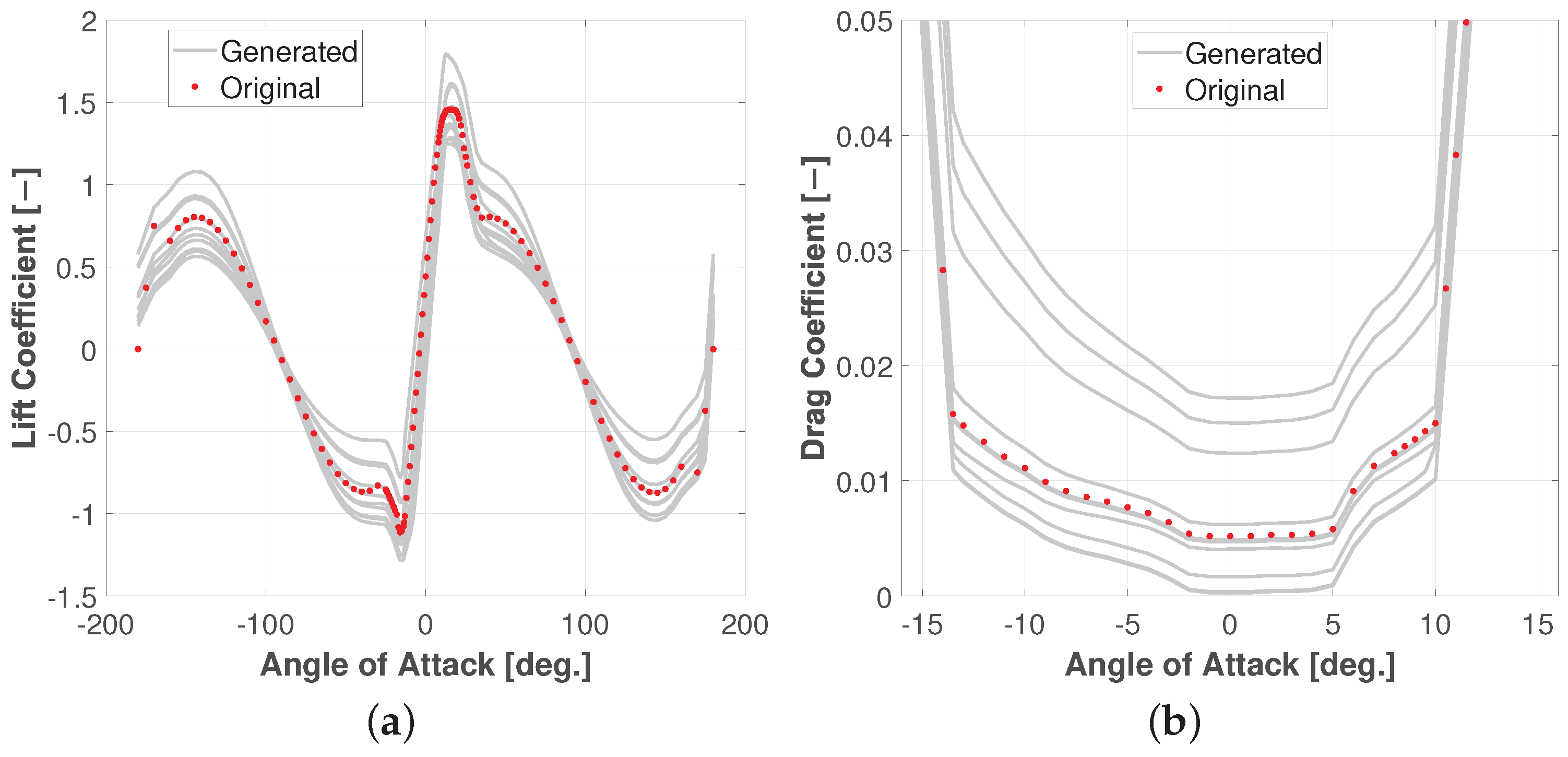
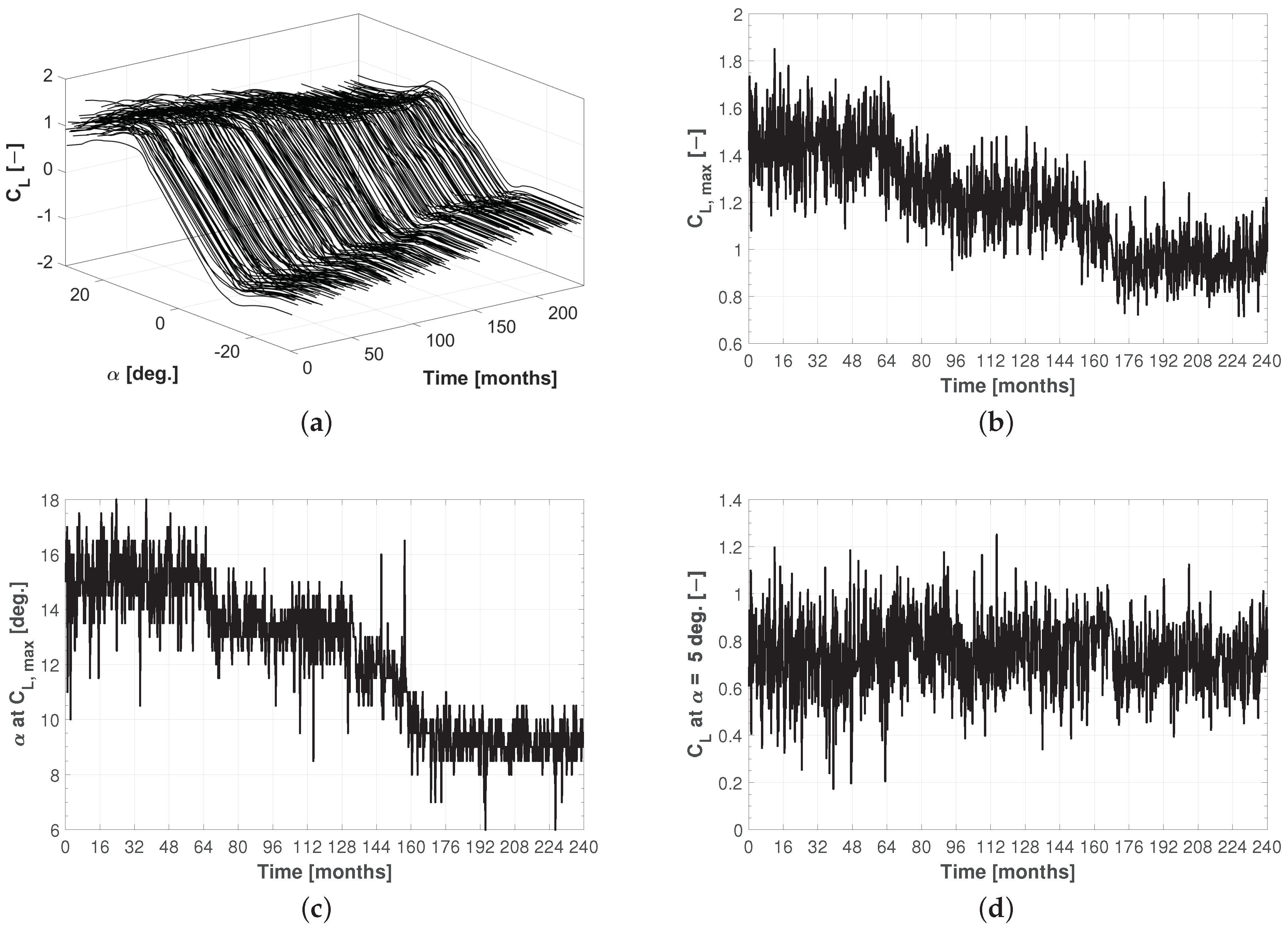
3.2. Stochastic Aerodynamic Polars Model

In this section, we generated a stochastic ensemble of degrading airfoil aerodynamic polars for use in forward aero-servo-elastic simulations. The outputs of the NHCPP were the degradation paths describing different degradation zones along the span of the rotor blades. Each arriving shock at a given time along these paths corresponds to a jump of a certain magnitude in the leading edge erosion severity. A jump in the erosion severity corresponds implicitly to a degradation of the aerodynamic properties of the airfoils affected by erosion along the span of the blade(s). However, uncertainties in the degrading airfoil aerodynamics lift and drag coefficients curves still remained to be accounted for. Our proposed LEE model hence takes into account the inherent uncertainty in airfoil static lift and drag coefficients during the erosion period via a stochastic model of static airfoil lift and drag polar curves. The details of this model can be found in Abdallah et al. [58], with a short summary presented herein for brevity.

Lift and drag coefficients are affected by several sources of uncertainty: uncertainties related to wind tunnel airfoil testing, 3D-flow correction uncertainties, surface-roughness uncertainties, uncertainties related to deformations in the blade geometry (during manufacturing and handling or deflections induced under load), uncertainties stemming from Reynolds number effects, uncertainties related to post-stall extrapolation of airfoil characteristics, and finally uncertainties resulting from prototype testing. The joint distribution of all these random variables cannot be quantified, and, therefore, a stochastic model was used as suggested in [58]. In this model, the lift coefficient was parametrized by the slope in the linear range $\frac{\partial C_L}{\partial \alpha }$, the point of maximum lift $\left(Ao{A}_{max},C_{L,max}\right)$, the point indicating the start of the trailing edge separation $\left(Ao{A}_{TES},C_{L,TES}\right)$ and the point where the stall recovery is initiated $\left(Ao{A}_{SR},C_{L,SR}\right)$. This model also includes the parametrization of the drag coefficient through a bias at low angles of attack and by the maximum drag coefficient point at $AoA=\pm {90}^{\circ }$, where the largest variation was observed. Figure 6 shows samples of the stochastic lift and drag coefficients for $NACA64618$ for an erosion of severity class 5. Based on these perturbations, modified $C_L$ and $C_D$ curves were produced that preserved the main characteristics of the reference curves but yielded magnitudes and features that reflect possible uncertainties related to the aerodynamic properties of the airfoil section under actual conditions.

Putting it all together, the NHCPP coupled to the generator of stochastic ensembles of aerodynamic polars yields realistic degrading aerodynamic polars over the degradation time horizon, for every degrading zone and airfoil section on the rotor blades. For example, Figure 7a shows the degrading $C_L$ over a 20-year period (240 months) for for $NACA64618$ airfoil, and Figure 7b represents the corresponding degrading max lift coefficient. Figure 7c,d show the degrading angle of attack at max lift coefficient and the degrading lift coefficient at $\alpha =5^{\circ }$, respectively.

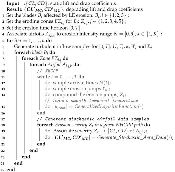
3.3. Overview of the Algorithm

The main ingredients of the model included a (1) spatio-temporal stochastic damage process and (2) a generator of stochastic ensemble of degrading airfoil aerodynamic polars. The algorithm is summarized in Algorithm 1.

Algorithm 1: Spatio-temporal stochastic model of leading edge erosion.

4. Uncertainty Modeling and Aeroelastic Simulations

Two categories of uncertain random variables (RV) were considered: wind inflow and aerodynamic effects. We elaborated on the aerodynamic uncertainties in the previous section. In this section, we detail the wind inflow uncertainties and the aeroelastic simulations setup. The conventional wind turbine structural damage computation process utilizes aeroelastic load simulations for wind turbines under normal and extreme operation and wind inflow turbulence conditions, whereby the extreme and fatigue load cycles determined over a short period of time at each mean wind speed are extrapolated over the full expected lifetime. Such a process does not consider the changes in inflow and environmental changes over long time periods, which are indeed relevant to the LEE process.

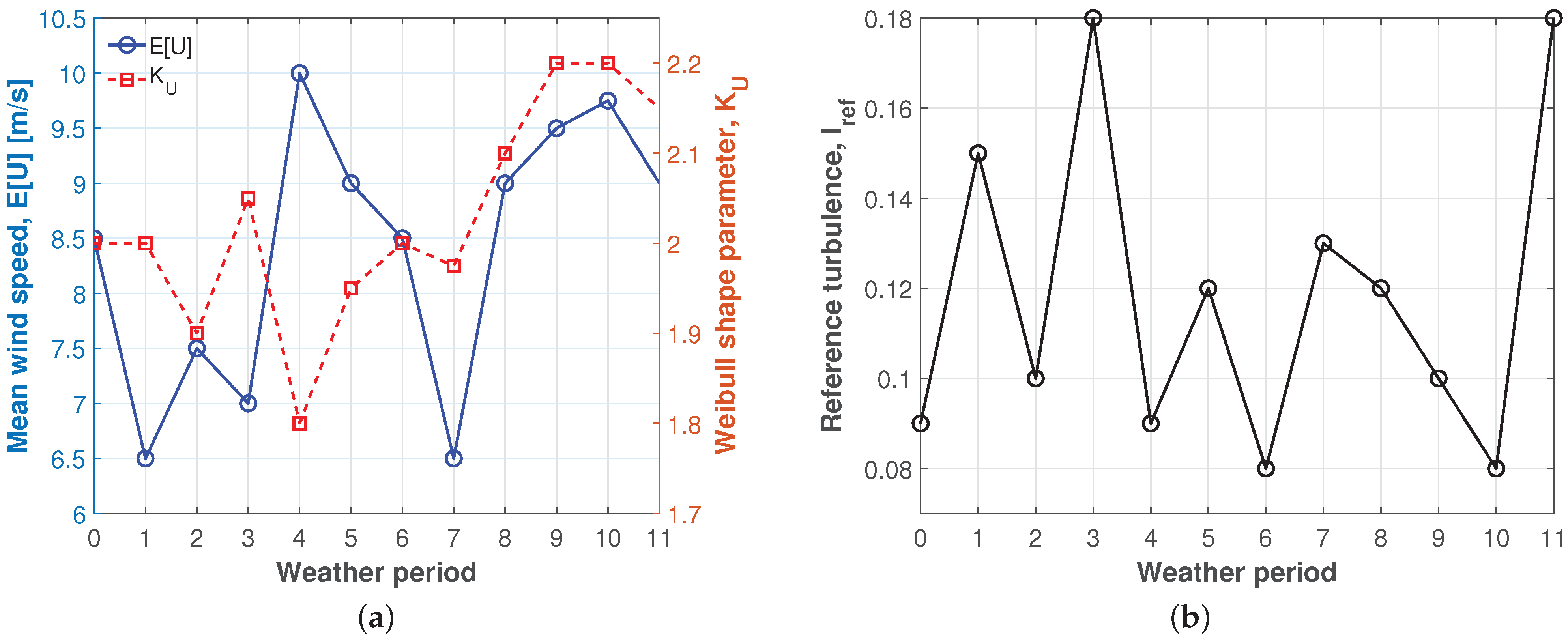
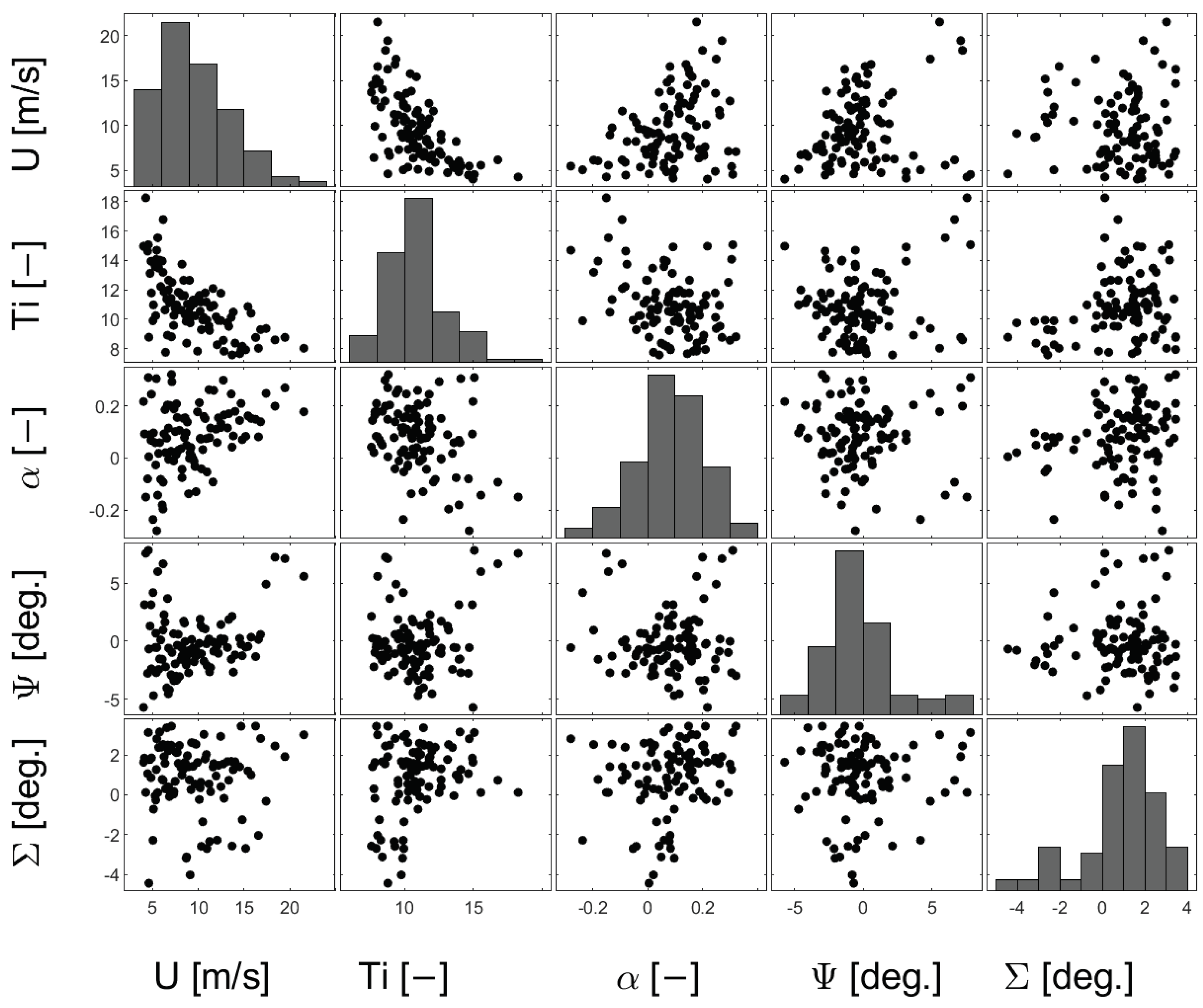
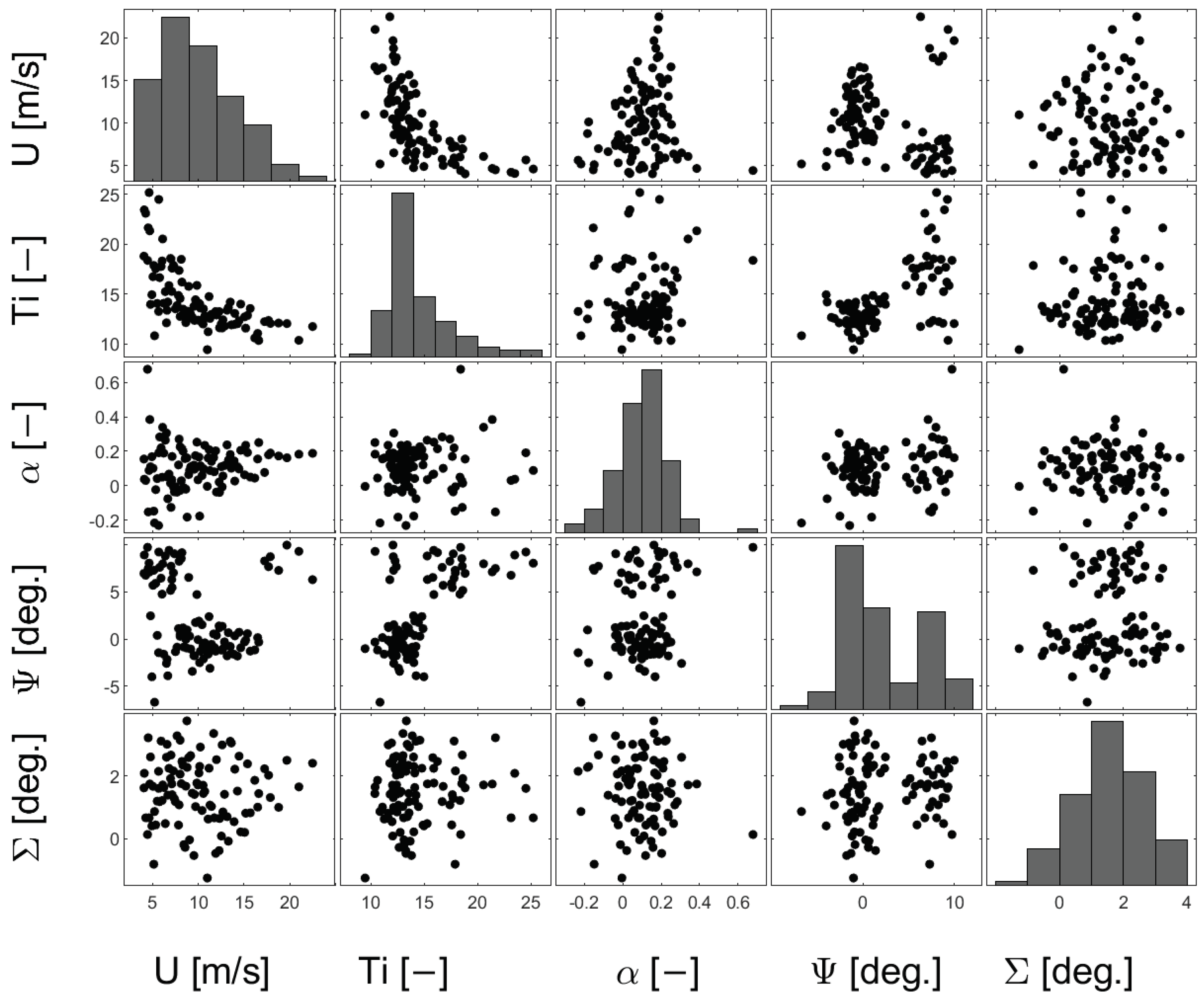
4.1. Stochastic Models of Inflow RVs

In turbulent inflow conditions, the structural dynamic response of wind turbines is highly influenced by factors such as average wind speed, turbulence intensity, wind shear, and skewness of the inflow. Taking these influences into account, our simulations were set up with the following RVs: turbulence intensity, $T_i$, mean wind speed, U, wind shear, $\alpha$, horizontal inflow skewness, $\mathsf{\Psi }$, and the vertical inflow skewness, $\mathsf{\Sigma }$.

A Weibull distribution describes the mean wind speed, truncated to (4–25) m/s, with the following parameters:

$$\begin{array}{c}\hfill \begin{array}{cc}\hfill \mathbb{E}\left(U\right)& =8.5,where{A}_U=\frac{2\times \mathbb{E}\left(U\right)}{\sqrt{\pi }}\hfill \\ \hfill K_U& =2.0\hfill \end{array}\end{array}$$

(4)

The normal turbulence model, defined in the wind turbine design standard [64], describes the conditional dependence between the mean wind velocity U and the turbulence ${\sigma }_U$. We chose to utilize $I_{ref}=0.16$ as the value for reference ambient turbulence intensity, which was the expected value of the turbulence intensity at 15 m/s. The local statistical moments of ${\sigma }_u\sim \mathcal{LN}\left({\mu }_{{\sigma }_U},{\sigma }_{{\sigma }_u}^2\right)$ determine this conditional dependency as:

$$\begin{array}{c}\hfill \begin{array}{cc}\hfill \mathbb{E}\left({\sigma }_u\mid U\right)& =I_{ref}\left(0.75u+3.8\right)\hfill \\ \hfill \mathbb{V}\left({\sigma }_u\mid U\right)& ={\left(1.4I_{ref}\right)}^2\hfill \end{array}\end{array}$$

(5)

As a result, we can express the turbulence intensity as: $T_i=\frac{{\sigma }_u}{u}$.

A power-law relationship describes the wind profile, by defining the average wind velocity u at height Z above ground with respect to the reference mean wind speed $u_h$, measured at hub height $Z_h$:

$$\begin{array}{c}\hfill \frac{u}{u_h}={\left(\frac{Z}{Z_h}\right)}^{\alpha }\end{array}$$

(6)

where $\alpha$ is the shear exponent. The conditional dependence between the wind shear exponent $\alpha \sim \mathcal{N}\left({\mu }_{\alpha },{\sigma }_{\alpha }^2\right)$ and the mean wind speed U is expressed as [65]:

$$\begin{array}{cc}\hfill \mathbb{E}\left(\alpha \mid U\right)& =0.088\left(ln\right(u)-1)\hfill \\ \hfill \mathbb{V}\left(\alpha \mid U\right)& ={\left(\frac{1}{u}\right)}^2\hfill \end{array}$$

(7)

We introduced a custom conditional dependence between the average wind velocity U and the inflow horizontal skewness $\mathsf{\Psi }$, truncated to $(-11,11)deg.$, $\mathsf{\Psi }\sim \mathcal{N}\left({\mu }_{\mathsf{\Psi }},{\sigma }_{\mathsf{\Psi }}^2\right)$:

$$\begin{array}{c}\hfill \begin{array}{cc}\hfill \mathbb{E}\left(\mathsf{\Psi }\mid U\right)& =ln\left(u\right)-3\hfill \\ \hfill \mathbb{V}\left(\mathsf{\Psi }\mid U\right)& ={\left(\frac{15}{u}\right)}^2\hfill \end{array}\end{array}$$

(8)

The conditional dependence between the average wind velocity U, the turbulence intensity $T_i$, and the vertical inflow skewness $\mathsf{\Sigma }$, truncated to $(-6,6)deg.$, was proposed such that:

$$\begin{array}{c}\hfill \mathsf{\Sigma }\sim \mathcal{N}\left({\mu }_{\mathsf{\Sigma }},{\sigma }_{\mathsf{\Sigma }}^2\right):\left\{\begin{array}{cc}{\mu }_{\mathsf{\Sigma }}=-2,{\sigma }_{\mathsf{\Sigma }}^2=1.0,\hfill & \mathrm{if}{T}_i\le 10\%\&\alpha \le 0.1.\hfill \\ {\mu }_{\mathsf{\Sigma }}=1.5,{\sigma }_{\mathsf{\Sigma }}^2=1.0,\hfill & \mathrm{otherwise}.\hfill \end{array}\right.\end{array}$$

(9)

The blade leading-edge degradation scenario occured over a 240-months period; consequently, we introduced an additional element of uncertainty by allowing a time-varying aspect of the inflow conditions, namely, the mean wind speed $\mathbb{E}\left(U\right)$, the shape parameter $K_U$ of the Weibull distribution, and the reference ambient turbulence intensity $I_{ref}$, as shown in the example in Figure 8.

By generating samples with the Sobol quasi-random sequences, the wind inflow and aerodynamic RVs were sampled uniformly over the unit hypercube, i.e., as evenly as possible over the multi-dimensional input space [66]. Over the degradation period, 1200 joint samples of the wind inflow RVs were sampled, as shown in Figure 9 and Figure 10. We generated a realization of the inflow turbulent wind field time-series by sampling U, ${\sigma }_U$, $\alpha$, $\mathsf{\Psi }$, and $\mathsf{\Sigma }$, which, together with a sample of the stochastic lift and drag coefficients, formed the input to the OpenFAST aero-servo-elastic simulator. Using this simulator, we could then compute the aeroelastic response of the wind turbines structure under continuous erosion of the blade’s leading edge.

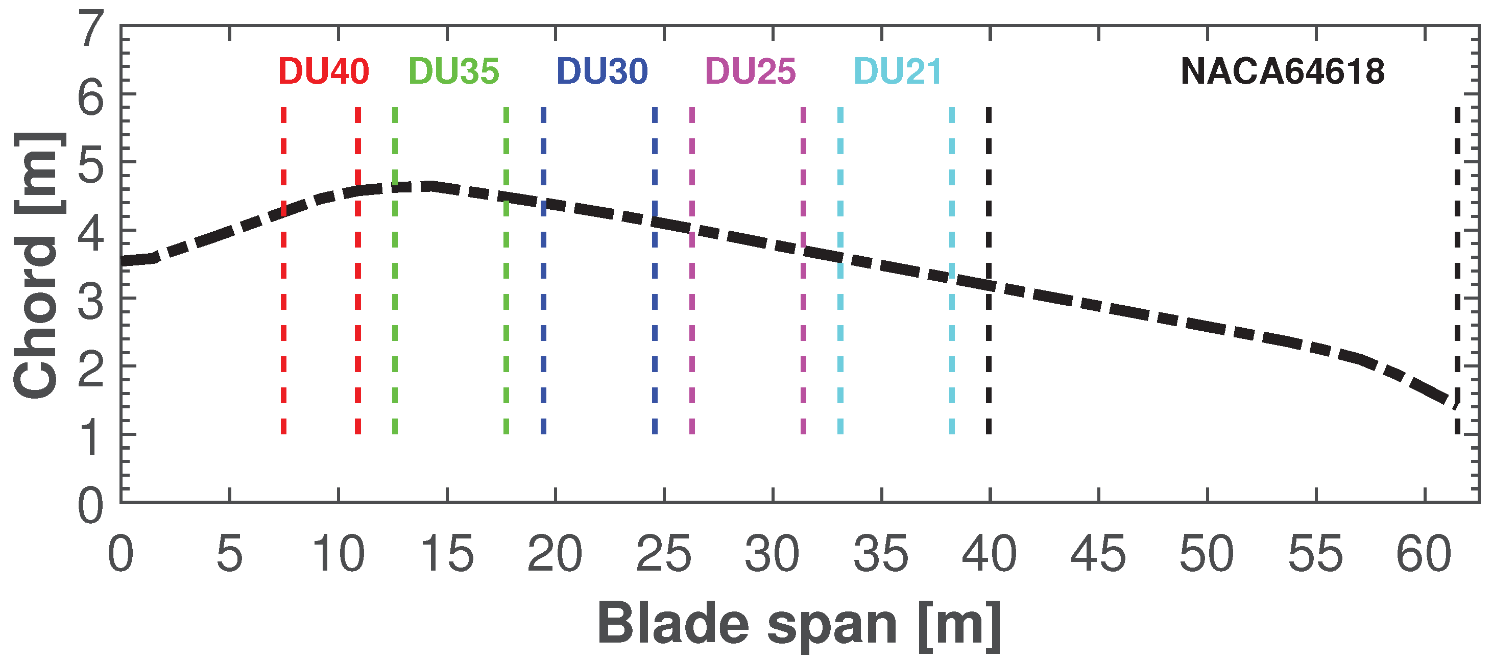
4.2. Setup of the Aero-Servo-Elastic Simulations

Our coupled aero-servo-elastic simulations with the proposed NHCPP leading-edge degradation model was based on the OpenFAST simulator. OpenFAST [67] is a coupled aero-hydro-servo-elastic analysis tool for modeling wind turbines. The primary use of OpenFAST is to run nonlinear time-domain simulations. We elected to simulate in OpenFAST the NREL reference 5 MW wind turbine [68], which is a well-documented three-bladed up-wind horizontal-axis wind turbine, with a rotor diameter of 126 m and a 90 m hub height. The layout of the airfoils along the span of the blade is shown in Figure 11.

Using blade element momentum theory as the basis for the aerodynamic model, the OpenFAST simulator includes dynamic stall, skewed inflow, and generalized dynamic wake. Aerodynamic forces are computed by interpolating from lookup tables composed of provided aerodynamic polars. In our case, the aerodynamic polars correspond to the degrading lift and drag coefficients generated in the NHCPP, such as the one shown in Figure 7a. The Kaimal turbulence model [69] was utilized in OpenFAST to compute the stochastic input wind field. In our setup, we assigned a maximum of five independent zones that undergo leading-edge erosion per blade. The location of the degradation zones, normalized by the blade length, along the span of the blades were:

$$\begin{array}{c}\hfill EZ:(0.65,0.68),(0.70,0.80),(0.82,0.85),(0.87,0.90),(0.92,1.00)\end{array}$$

We simulated 20 years (240 months) worth of wind turbine operation with blades’ LEE. We generated one sample every (approximately) six days, resulting in a total of 1200 simulated samples. Every sample was a 600-s multi-variate time series with 228 sensor signals each, sampled at 100 Hz. A few examples of the time series signals are shown in Figure 12.

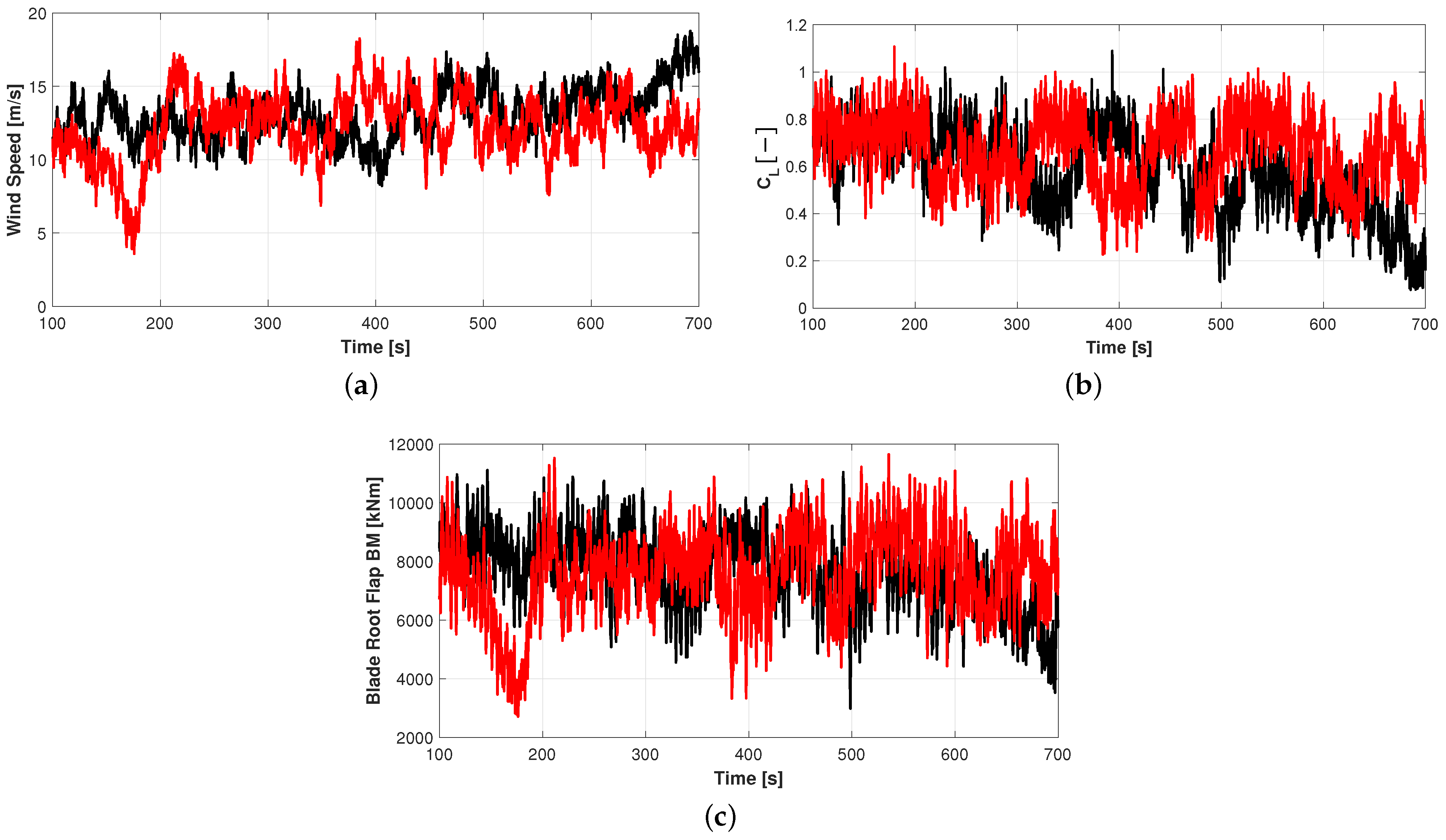
4.3. Retained Output from Aero-Servo-Elastic Simulations

As mentioned in Section 1, this research was motivated by the development of an aero-acoustic measurement system that can be used for SHM tasks. In this simulated setup, we assumed one measurement node located at 0.96 of the blade length, located within Eroding Zone 5 (near the tip of the blade). From our aero-servo-elastic simulations, we elected to retain those output signals, which are expected to emanate from the aero-acoustic measurements nodes, namely, lift and drag coefficients, angle of attack, and wind speed as listed in

Table 3. Output sensors of the aero-servo-elastic simulations retained for diagnostics.

Sensor Name	Description
$Time$	Time steps of the simulations
$Wind1VelX$	X-direction wind velocity at hub-height
$B1N9Cl$	Lift force coefficient at Blade 1, Aerosense Node at $0.96R$
$B1N9Cd$	Drag force coefficient at Blade 1, Aerosense Node at $0.96R$
$B1N9Alpha$	Angle of attack at Blade 1, Aerosense Node at $0.96R$

.

5. Diagnosing LEE via Transformers

The simulation pipeline described above allowed us to generate data that replicate the sensory output of Aerosense nodes. Thus, we were able to produce datasets to train a deep learning method, with the end goal being to detect and estimate the extent of leading-edge erosion on wind turbine blades. We chose to implement a modified version of a popular class of sequential deep learning models: Transformers [39].

To motivate the diagnostics task, we considered the case where $C_L$ time-series signals emanate from two sections along the span of the blade. Figure 13a shows a scatter plot of time series of $C_L$ at sections $0.96R$ vs $0.75R$ of the blade for wind speeds varying between 6–16 m/s and no LEE (clean blade). Figure 13b shows a similar plot for a fixed wind speed 11 m/s and evolving severity of leading-edge erosion at section $0.96R$. An important property is that the relational dependency of the $C_L$ between the two sections will change over time either due to changes in the severity of the leading-edge erosion or due to short-term variation in inflow and operating conditions. The problem is thus to detect leading-edge erosion and its severity, which could be regarded as a problem of finding the optimal discriminants for erosion versus other effects (inflow, operational conditions, aerodynamic uncertainties, etc.) from multivariate time-series response signals.

The following are aspects we built into the diagnostics method for LEE classification, taking into account the nature/circumstance of an operating wind turbine in the field:

• Labeled data for LEE are hard to acquire and are scarce; as a result, any method must be designed not to suffer from over-fitting under scarce labeled data availability.
• Diagnostics shall be done with remote streaming of sensor data. Human intervention and turbine down-time should be alleviated.
• The data used in the diagnostics method intend to emulate the sensory output of a single MEMS-based aerodynamic and aero-acoustic measurement node positioned in proximity to the tip of the wind turbine blade.
• The method shall be capable of ingesting 10-min-long multivariate time-series (industry standard SCADA recording length), sampled at 100 Hz, resulting in 60,000 data-point-long sequences. A sampling rate of 100 Hz may seem excessive, but the aim is to capture even small turbulence scales.
• A supervised scheme shall be used to train a Transformer-based network by utilizing labeled data resulting from aeroelastic simulations of a turbine combined with the degradation model, as presented earlier in the article.
• Physics-constraints shall be built into the loss or likelihood function.
• The output predictions should be probabilistic in nature.

5.1. Experiments and Datasets

We utilized multivariate time-series data generated via the coupled simulation pipeline previously described. The designation multivariate stems from treatment of multiple variables, referring to signals pertaining to lift, drag, angle of attack, and inflow velocity, which are recorded via an Aerosense node located near the blade tip. On the other hand, the term multivariate could further refer to the use of multiple Aerosense stations at different locations along the span of the blade(s); this, however, lies beyond the scope of the present work. After some initial testing, we opted to utilize the four variables shown in Table 3 as inputs to the Transformer. For instance, no performance benefit was found when including simulated acceleration data.

Three sets of experiments, each with different data requirements, were performed aiming to answer the following questions:

• Are we able to learn the LEE severity classes from aerodynamic MTS data, in the general machine learning sense, with balanced data classes and no prior knowledge?
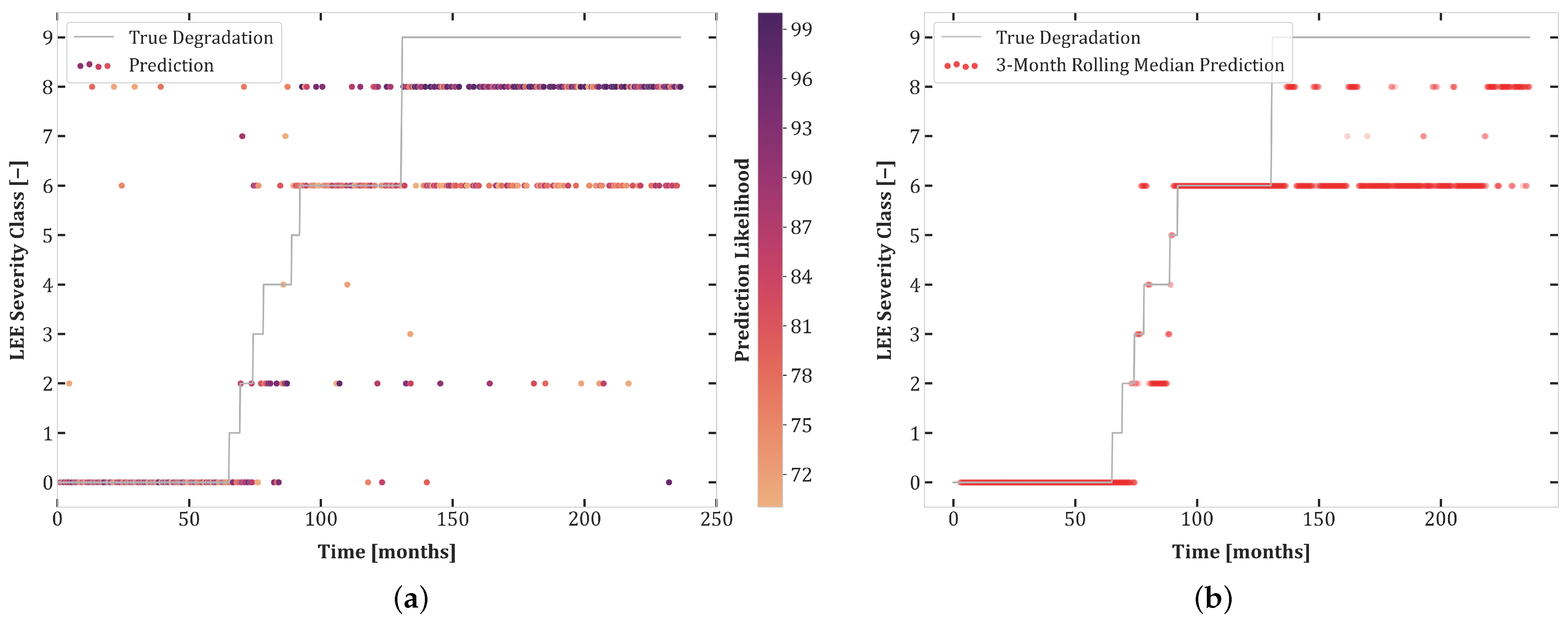
• In a continuous monitoring context, are we able to diagnose jumps in LEE severity and therefore identify the degradation path that the system takes?
• Are we able to do so in a realistic setting, with all previously described sources of uncertainty present in the simulations?

Thus, the goal of the first set of experimental tasks was to train the neural network on a generalized dataset with reduced uncertainty and where each degradation class appeared in equal measure. This is not representative of a real degradation path, where the inherent stochasticity of the NHCPP may result in some classes appearing very briefly, but we aimed to avoid biasing the network towards a random predominant class. Moreover, this set of experiments also aimed to understand how data availability affects classification performance and how separable the classes are. Two datasets, corresponding to Experiments 1.1 and 1.2, were generated: one with the full 10 severity classes and one with a reduced amount of severities (levels 0, 1, 6, and 9). For this set of experiments, no information on previous states was used. In each of the sub-experiments, 4800 aero-elastic simulations were gathered, then split into train, validation, and test sets in a 70/20/10 split.

The second set of experiments aimed to assess whether using full degradation paths in a continuous monitoring setup to train the diagnostics method is a suitable strategy. Here, the datasets were comprised of full NHCPP degradation paths, albeit with reduced uncertainty. Due to the stochastic degradation, the datasets did not have balanced classes. Assuming that a continuous monitoring system is in place, we therefore had access to the previous degradation states. This allowed for degradation monotonicity to be enforced in the prediction, thus constraining the output to physically possible solutions (i.e., it is physically impossible to have a state that is less degraded than previous states—except for the case of direct service intervention for repair and maintenance, which is out of scope in this work). Another objective was to evaluate whether severity grouping is a viable strategy. Indeed, grouping the LEE stages by type (see Table 1) could be beneficial as a coarse predictor, if it proves to be sufficiently accurate. Thus, in Experiment 2.1, all 10 degradation levels were used as labels, while, in Eperiment 2.2, the levels were grouped by type. Three full NHCPP degradation paths (new sample every six days, over a 20-year period) with 1200 simulations each were separated into training and validation sets in a 80/20 split. A full degradation path, with 1200 data points, was reserved as the test dataset for final evaluation.

The goal of the third set was to evaluate how the model would perform in a realistic continuous monitoring situation. Here, the dataset was also made of full NHCPP simulations, but in this case, all possible stochasticity was turned on. Again, we assumed that we had access to the previous degradation states. We also evaluated class grouping, separating the experiment into two. Three full NHCPP degradation paths (new sample every six days, over a 20-year period), each consisting of 1200 MTS data points, were divided into training and validation sets based on a 80/20 split. The test dataset was comprised of one full degradation path, with 1200 data points also unused in training or validation.

Table 4. Dataset properties of the different diagnostic experiments.

Parameter	Experiments
	1.1	1.2	2.1	2.2	3.1	3.2
NHCPP severities	0–9	0, 1, 6, 9	0–9	0–9	0–9	0–9
Severity type grouping	-	-	-	0, A, B, C	-	0, A, B, C
Stochastic degradation	-	-	✓	✓	✓	✓
Inflow turbulence	✓	✓	✓	✓	✓	✓
Aerodynamic uncertainty	-	-	-	-	✓	✓
Weather variability	-	-	-	-	✓	✓
Num. training samples	3360	3360	2880	2880	2880	2880
Num. validation samples	960	960	720	720	720	720
Num. testing samples	480	480	1200	1200	1200	1200

summarizes the differences between the datasets of the three sets of experiments, including the partition of data between the different subsets.

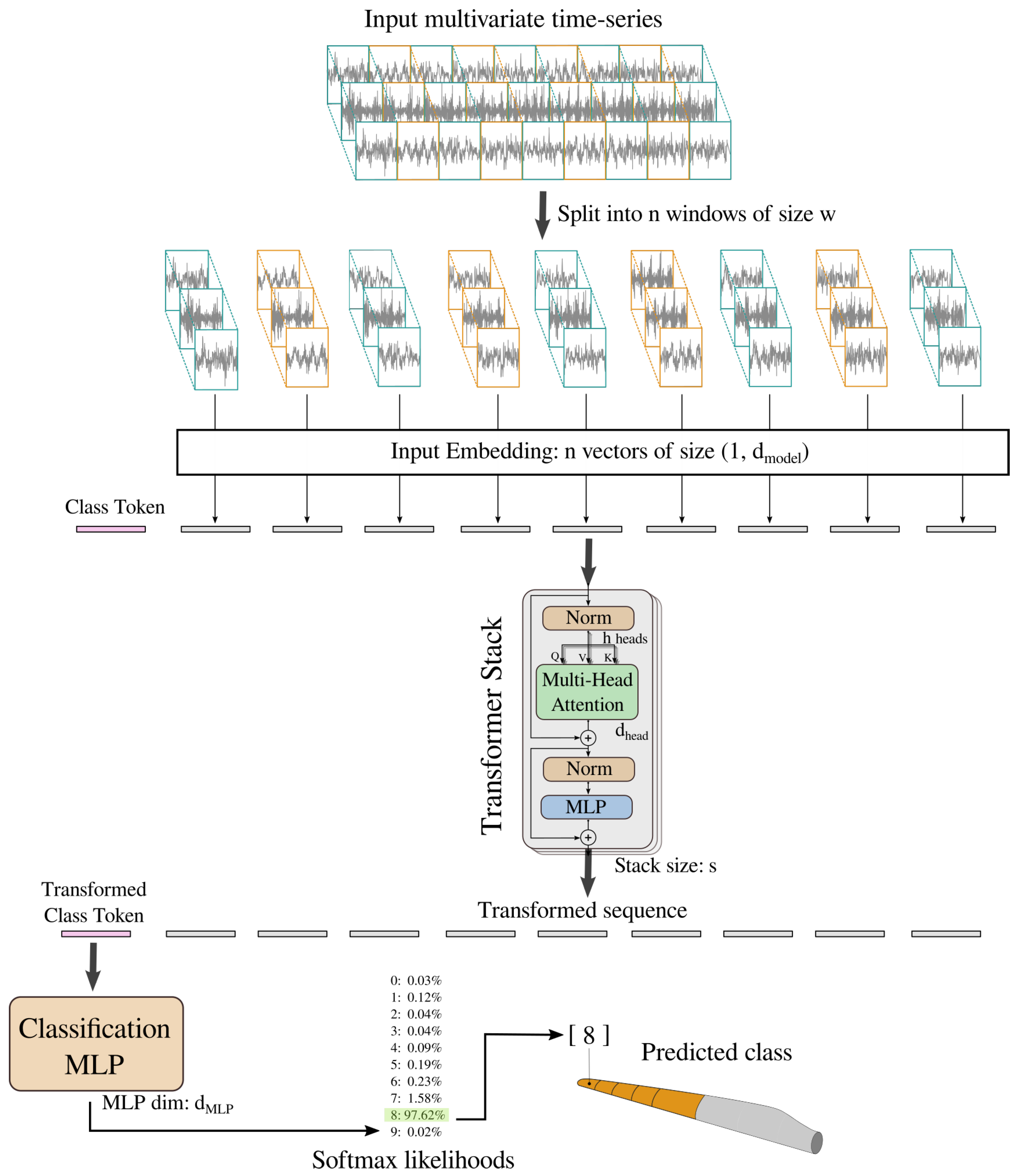
5.2. Transformer Architecture

Here, we introduce the architecture of our Transformer neural network, used to classify long-sequence multivariate time-series data and infer the degradation status of the leading edge.

Transformers are models that rely on self-attention mechanisms to highlight and learn dependencies within sequences. Typically, self-attention is implemented by parsing the input sequence into into key (K), query (Q), and value (V) vectors. The attention weights on the values are then obtained by taking the scaled dot products of the query with all keys and then by applying a softmax function. Using the classical notation [39], this writes:

$$\begin{array}{c}\hfill \mathrm{Attention}(Q,K,V)=\mathrm{softmax}\left(\frac{Q{K}^T}{\sqrt{d_k}}\right)V\end{array}$$

(10)

where $d_k$ is the dimension of the key and query vectors and is used to scale the dot product. In practice, h-scaled dot-products are used in parallel, within multi-head attention layers. A multi-head model is able to attend jointly to information gathered from different parts of the input, providing an improvement in representation over a single attention mechanism. The final attention vector is obtained by concatenating each of the dot-product results:

$$\begin{array}{c}\hfill \mathrm{MultiHead}(Q,K,V)=\mathrm{Concat}(hea{d}_1,\cdots ,hea{d}_h)W^O\end{array}$$

(11)

with

$$\begin{array}{c}\hfill hea{d}_i=\mathrm{Attention}(Q{W}_i^Q,K{W}_i^K,V{W}_i^V)\end{array}$$

(12)

where $W_i^Q\in {\mathbb{R}}^{d_{\mathrm{model}}\times d_k}$, $W_i^K\in {\mathbb{R}}^{d_{\mathrm{model}}\times d_k}$, $V_i\in {\mathbb{R}}^{d_{\mathrm{model}}\times d_v}$ and $W^O\in {\mathbb{R}}^{h·d_v\times d_{\mathrm{model}}}$ are parameter matrices.

Multi-head attention layers are combined with fully connected networks and layer normalization to form the base architecture of each layer of the Transformer stack. We used a novel time-windowing Transformer model, which is based on the patch system used in the Vision Transformer (ViT) model [40]. This architecture, as shown in Figure 14, aims to address the quadratic attention bottleneck, an obstacle that limits the length of sequences a Transformer can use. Indeed, the computational complexity of the self-attention layers in Transformer models scales as $\mathcal{O}\left(L^2\right)$, where L is the length of the input sequence. Given our requirements, the input time-series had a length of L = 60,000, which is prohibitively resource-intensive for standard Transformer models. To alleviate this issue, we proposed to divide the data into N windows along the time-dimension before passing each window through the learnable input embedding. This allowed us to use the full input time-series without resorting to downsampling, which would entail losing information.

Before dividing the MTS into windows, each of the individual channels/variables was normalized in time. Then, the input embedding encodes each time-series window into a vector of size $d_{\mathrm{model}}$, which is the latent size used throughout the Transformer. The type of input embedding used has a considerable impact on performance, and many embedding types can be envisaged. We chose to use a learnable linear embedding for simplicity, based on initial testing and the literature [40]. A class token is concatenated to the embedded sequence such that its state at the output of the Transformer is used to infer the degradation severity. Class tokens are commonly used in NLP tasks [70] and are an effective way to retrieve categorical information from Transformers. Traditionally, positional encodings are then added to the sequence in order to instill directional information into the model. Contrary to standard NLP Transformer models, we did not use a positional encoding. Two positional encoding methods were tested (classical sine functions and simple linear encoding); however, both of these methods hindered classification performance.

The classification head consists of a single hidden layer multilayer perceptron (MLP) that processes the class token at the output of the Transformer. It outputs a vector with a size equal to the number of possible degradation classes, which, when passed through a softmax activation, gives the likelihood scores of each class. For each class output $x_i$, the softmax likelihood writes:

$$\begin{array}{c}\hfill \mathrm{softmax}\left(x_i\right)=\frac{\exp \left(x_i\right)}{{\sum }_j^{}\exp \left(x_j\right)}\end{array}$$

(13)

If we aim to predict the degradation at multiple zones along the blade, we can simply stack multiple MLPs, one for each zone.

Table 5. Parameters of the Transformer architecture.

Parameter	Value
Number of windows, n	300
Window size, w	200
Internal Transformer dim., $d_{model}$	256
Transformer stack size, s	6
Num. self-attention heads, h	8
Self-attention head dim., $d_{head}$	64
Output MLP dim., $d_{MLP}$	2048

summarizes the values used in the Transformer architecture.

5.3. Loss Functions

We first trained and evaluated the Transformer model on the datasets with equal amounts of degradation classes, in the sense of a traditional classification problem. Thus, the objective function for this first task was the standard cross-entropy loss:

$$\begin{array}{c}\hfill {\mathcal{L}}_{CE}(\mathbf{y},\widehat{\mathbf{y}})=-\sum _{i=1}^{\mathrm{n}}{y}_{i}log\left({\widehat{y}}_i\right)\end{array}$$

(14)

where $\mathbf{y}$ is a one-hot label vector indicating the correct class, $\widehat{\mathbf{y}}$ is a vector containing the predicted softmax probabilities for each class, and $\mathrm{n}$ is the number of classes.

In the second and third set of experiments, it was assumed that the state of the system is known for the previous sampling period. We used this information to enforce physicality; we added a second term to the loss function that penalizes a predicted degradation class that is lower than the known previous class. This second term is the margin ranking loss:

$$\begin{array}{c}\hfill {\mathcal{L}}_{MR}(\widehat{\mathrm{c}},{\mathrm{c}}_{\mathrm{prev}})=-\max (0,\widehat{\mathrm{c}}-{\mathrm{c}}_{\mathrm{prev}}+\mathrm{m})\end{array}$$

(15)

where $\widehat{\mathrm{c}}$ is the predicted class, ${\mathrm{c}}_{\mathrm{prev}}$ is the degradation class of the previous known state, and $\mathrm{m}$ is the margin hyperparameter. Overall, the objective function for the second and third experiments was therefore:

$$\begin{array}{c}\hfill {\mathcal{L}}_{tot}={\mathcal{L}}_{CE}+\alpha {\mathcal{L}}_{MR}\end{array}$$

(16)

where $\alpha$ is a hyperparameter used to balance the two components.

5.4. Training Regime

During training, we used a batch size of 20 along with the Adam optimizer [71] with parameters ${\beta }_1=0.9$, ${\beta }_2=0.999$, $ϵ={10}^{-8}$, and a learning rate of $lr=5·{10}^{-5}$ to perform stochastic gradient descent. After 40 epochs of training, the learning rate decayed by a factor of $0.2$. To ensure that the trained model is able to generalize well, and does not overfit, dropout with a 0.3 rate was used in the attention, fully-connected, and embedding layers. Furthermore, training and validation metrics (loss and accuracy) were monitored throughout the training sequence, allowing us to halt training without overfitting. We found that for most experiments, training for around 60 to 120 epochs was sufficient.

6. Results

For each diagnostic experiment, a Transformer model was trained on the training dataset, monitored on the validation dataset, and final evaluation took place on the test dataset. All model hyperparameters were static throughout the experiments, and only the number of training epochs varies, as we choose the epoch with the best validation performance. We report in the following sections the results for all three sets of experiments gathered on the previously unseen test dataset.

6.1. Experiment Set 1

The first set of experiments aimed to assess the potential of the Transformer for diagnostics given ideal conditions: a balanced data set where each individual degradation class appears in equal measure.

Table 6. Testing classification accuracy of Experiments 1.1 and 1.2.

Experiment	Testing Accuracy (%)
	All Predictions	>70% Likelihood
Exp. 1.1	66.67	72.65
Exp. 1.1 Large	80.63	85.56
Exp. 1.2	96.04	97.22

reports the testing accuracy scores gathered for Experiments 1.1 and 1.2. We note a significant difference between the results of the two experiments, where the 4-class setup outperformed the 10-class setup by 30% in terms of test accuracy. Knowing that Transformers are data-intensive models that respond well to large datasets, this discrepancy can be partly explained by accounting for the number of simulations per individual class. Indeed, as both training sets have the same total number of samples, there are 2.5 times the amount of samples per severity class in Experiment 2.2. To factor out the disparity in the amount of data per class, we generated a large version of training dataset of Task 1.1, with a total of 10,176 training samples and 2544 validation samples. In this experiment (1.1 large), the number of training samples per class was larger than for Experiment 1.2 (1017 versus 840), yet the 4-class model still outperformed the 10-class model by over 16%. In general, it is advantageous to train on larger amounts of severity classes from a risk management perspective, as it allows for more optimal maintenance intervention schemes. However, as highlighted above, a fine-grained approach requires more training data in order to diagnose accurately with high confidence and could result in higher amounts of false positives, which could then lead to an increase in operation and maintenance ($O\&M$) costs. Thus, there is a trade-off between risk minimization via fine-grained diagnostics of LEE severity and increased costs due to higher amounts of false positives and requirements for larger training datasets, which can be optimized to meet risk management policies and budgetary specifications.

The difference in accuracy can also be explained by the separability of the individual severity classes. We show in Figure 15 the confusion matrices generated on the test sets for Experiments 1.1. and 1.2. It can be noted that the Transformer model was able to successfully differentiate between the lowest and highest of erosion severities, as demonstrated by the lack of misclassified samples with large differences in severity. Similar LEE erosion classes exhibited higher amounts of wrongly classified samples. This aligned with our expectations: small increases in the level of erosion only marginally increased the roughness of the leading edge, which has a minor impact on blade aerodynamics. It is therefore more challenging to distinguish between similar LEE severities based on integrated pressure quantities.

6.2. Experiment Set 2

Here, we assess the use of stochastic degradation paths as diagnostic training points.

Table 7. Testing classification accuracy of Experiments 2.1 and 2.2.

Experiment	Testing Accuracy (%)
	All Predictions	>70% Likelihood
Exp. 2.1	65.42	78.41
Exp. 2.2	67.75	69.48

shows accuracy scores gathered on an un-seen degradation path for Experiments 2.1 and 2.2. Figure 16a plots the predicted states of each MTS data point alongside the true degradation path for the test dataset that contains a full NHCPP path with up to 10 possible LE severity classes. In addition, we show the prediction confidence of each model output based on its softmax likelihood. Figure 16b displays the median predicted severity using a three-month rolling window.

These results show that this approach is viable and that we were able to successfully detect the jumps in degradation severity with some limitations. The main issue with training on stochastic degradation paths is the data imbalance. Indeed, the training dataset contained a majority of points belonging to Classes 0, 8, and 9, while Classes 5, 6, and 7 were underrepresented. This is reflected in the results, where the accuracy was high for Class 0 but low for Classes 5 and 6. Moreover, the prediction confidence was, in general, lower for underrepresented classes. A possible solution to address this was to train on grouped severity classes. We evaluated this approach in Experiment 2.2 and plotted the resulting predictions in Figure 17. Overall, this approach yielded a higher prediction accuracy, but it is still limited. Grouping artificially creates a somewhat balanced set and reduces class sparsity; however, it also leads to increased intra-class heterogeneity. As a result, learning to set the boundaries between the classes becomes more difficult and dependent on the number and the separability of the groups. This is reflected in the disparity of the minimum 70% confidence accuracy results between Experiments 2.1 and 2.2. Indeed, the low intra-class heterogeneity of the 10-class approach results in low confidence predictions for ambiguous samples, while the same ambiguous samples are incorrectly classified with a high likelihood in the grouped approach due to the network accounting for high intra-class variance. There is a balance to be found between the accuracy gain and the increase in intra-class heterogeneity induced by class grouping, depending on the number of groups. Should grouping be desired, unsupervised clustering approaches should be envisaged, in order to find the optimal number of groups.

In Experiments 2.1 and 2.2, non-physical predictions were penalized via the additional loss term (see Equation (17)). The result of using this extra component is apparent in Figure 16a and Figure 17a: there are noticeably fewer misclassified points below the true degradation path than above it (11.5% vs. 23.08% for Experiment 2.1 and 6.67% vs. 25.58% for Experiment 2.2).

6.3. Experiment Set 3

In Experiments 3.1 and 3.2, we assessed how the diagnostics method performs on more uncertain degradation paths, with multiple sources of variability. Not only were there large class imbalances due to the stochastic degradation but aerodynamic uncertainty (see Figure 6) and long-term weather fluctuations made it challenging to distinguish between different LEE severities. Weather variability is not commonly used for long-term aero-elastic modeling in the wind energy industry and is somewhat unrealistic, but the goal was to understand the limitations of the Transformer model by making inference extremely challenging. We report in

Table 8. Testing classification accuracy of Experiments 3.1 and 3.2.

Experiment	Testing Accuracy (%)
	All Predictions	>70% Likelihood
Exp. 3.1	35.00	45.75
Exp. 3.2	54.67	65.22

the accuracy scores gathered on an un-seen degradation path for Experiments 3.1 and 3.2. Overall, classification accuracy was much lower than previous experiments, but using only a high confidence predictions yielded a larger boost in accuracy. This can be explained by the inherent stochasticity and the high intra-class variance of this dataset, which makes high likelihood predictions rarer.

Figure 18 shows how challenging this final task is, where we see many non-physical misclassified points and an overall low prediction confidence. Here, the data imbalance had a big impact on classification performance. As the training set does not contain any samples with an LEE Severity Class 9, the network was unable to predict this severity on the given test set. Given these harsh training conditions, it is unsurprising that performance was underwhelming. To mitigate this, class grouping by LEE type was again tested in Experiment 3.2 (see Figure 19). Compared to Experiment Set 2, the benefit of grouping classes was clear here: performance was improved by almost 20%. This indicates that class grouping is a viable approach if intra-class heterogeneity is high by default and some classes are completely underrepresented. Nevertheless, even the results for grouped classes are lackluster, indicating that other strategies should be examined to deal with the very imbalanced datasets induced by the stochastic degradation paths. For instance, one could consider conditional retraining methods. By modifying the architecture so that it outputs confidence metrics based on how similar a sample is to the training set, as implemented in [72], one could then launch re-training procedures if multiple test samples that are very dissimilar to the training space are encountered.

6.4. Transferability and Curriculum Learning

Here, we evaluated the transferability of the different experiments and assessed the use of curriculum learning [73] as a method to improve accuracy on difficult results. In a curriculum learning training setup, the network is progressively exposed to harder datasets. In our implementation, we first trained the model on the dataset from Experiment 1.1, then we progressively added the training data from Experiments 2.1 and 3.1. The benefits of this approach should be twofold: (1) the data-intensive Transformer model is exposed to a larger dataset, and (2) the weights of the model are fine-tuned on more challenging samples, which helps to avoid local minima during gradient descent.

Table 9. Transferability and curriculum learning results.

Training Set(s)	Test Accuracy (%)
	Set 1.1	Set 2.1	Set 3.1
Set 1.1	–	71.25	28.25
Set 2.1	65.00	–	29.42
Set 3.1	30.00	39.25	–
Set 1.1, then 2.1	77.71	83.50	20.33
Set 1.1, then 2.1 & 3.1	77.08	80.50	37.08

and

Table 10. Transferability and curriculum learning results, for high confidence predictions.

Training Set(s)	>70% Likelihood Test Accuracy (%)
	Set 1.1	Set 2.1	Set 3.1
Set 1.1	–	80.21	30.19
Set 2.1	77.11	–	32.86
Set 3.1	35.58	40.97	–
Set 1.1, then 2.1	81.35	87.29	20.52
Set 1.1, then 2.1 & 3.1	84.42	88.53	50.22

show the results of the different transferability and curriculum learning experiments.

We remarked the following:

• The high accuracy of transferability tests between Experiments 1.1 and 2.1 highlights the similarity of these datasets. Moreover, the balanced dataset of Experiment 1.1 improves the prediction quality for Set 2.1.
• Although both Sets 1.1 and 2.1 contained all degradation classes, networks trained on these sets do not transfer well to Test Set 3.1, undoubtedly due to the uncertainty included in this experiment.
• There was better transferability between Sets 2.1 and 3.1 than between Sets 1.1 and 3.1. This can be explained by the extra loss component which enforces monotonicity in the second and third sets of experiments.
• The first curriculum learning experiment (Set 1.1 then 2.1) yielded a large performance boost for Test Sets 1.1 and 2.1. This was to be expected due to the data-intensive nature of Transformers and the similarity between these sets.
• The first curriculum learning experiment reduced transferability to Set 3.1. This is an indication of a loss of capacity to generalize to ambiguous data.
• The best test results on Set 3.1 were obtained in the second curriculum learning experiment. This suggests that pretraining on sets with reduced stochasticity followed by fine-tuning on uncertain data is an effective approach.
• The second curriculum learning experiment yielded the best high confidence accuracy for Sets 1.1 and 2.1. Thus, adding difficult, stochastic data points of Experiment 3.1 to the training dataset helps with regularization, enabling the model to construct a better internal representation of each severity class.

The curriculum learning test, which includes the data from all experiments, led to the highest high-confidence accuracy for the 2.1 test set. As this set is representative of a degradation path with standard aero-elastic simulation practices, we have plotted these results in Figure 20.

7. Limitations and Discussion

In the presence of the availability of comprehensive historical data, as those that we aimed to collect via the Aerosense monitoring system, it would be possible to tune the proposed NHCPP model parameters and calibrate all assumptions and modeling choices and further develop our probabilistic model in order to emulate more closely deterioration due to leading-edge erosion on operating wind turbines in the field over long time horizons [74,75]. In addition, the impact of field data quantity and quality on model calibration and its implication on the generated NHCPP will need to be closely evaluated.

Similar to the NHCPP, the gamma process has also been traditionally used for modelling deterioration. The shocks in a gamma process follow a gamma distribution, although the increments in the process are assumed to be independent from each other. Unlike Poisson processes, in gamma processes, there are infinite jumps in a finite time period. This is why the former are suited for modeling sporadic shock-induced damage, while the latter suit continuous, monotonous, and gradual deterioration [76].

One interesting extension to our NHCPP macro degradation model is to further couple it to a micro-model that describes the relative velocity between particles (including their density and size) and the blade [11]. Subsequently, based on the site’s atmospheric conditions and the wind turbine’s operational settings, the erosion severity is calculated from the number of particles impacting the blade surface.

An important outcome of the diagnostic experiments is the fact that the Transformer model is data-intensive. Our results point to the fact that more data almost always aids in classification performance. Furthermore, training on balanced datasets is always desirable, but obtaining these is difficult in real monitoring scenarios as it would require gathering data from many systems undergoing different degradation paths. To overcome this difficulty, the coupled NHCPP aeroleastic simulation setup can be used to replicate realistic degradation and produce balanced training sets, which can then be augmented with real field data, in a similar manner to the curriculum learning experiments.

As mentioned in the literature review, feature-extraction learning methods are often preferred for MTS classification tasks owing to their higher precision. In this context, we tested the state-of-the-art MINIROCKET method [27] with 10k kernels, combined with a standard linear classifier at the output for our diagnostics problem. This yielded an accuracy of only $55.21\%$ on the test set of Experiment 1.1 and $68.96\%$ on the test set of Experiment 1.2. This highlights the fact that very long sequences are challenging to deal with, while many methods found in the literature are not optimized for such tasks. Furthermore, feature-extraction methods may encounter difficulty finding optimal features, due to the fact that this problem features a very slow degradation rate with no flagrant traits from one stochastic sample to another. On the contrary, Transformers are well suited for this kind of input, as the self-attention mechanisms are effective at filtering out unnecessary data while focusing on the parts of the signal that are important.

While the loss term added to penalize non-monotonicity of the degradation process does help to reduce non-physical predictions, it is not strictly enforced. Another option would be to enforce this condition in the softmax output layer. Although this method would most certainly improve accuracy, it would lead to error accumulation when implemented in the context of a continuous monitoring setup. With our approach, erroneous predictions can be ignored by using a rolling window for instance. The proposed model could, however, be further improved by additional tuning of the objective function. One such improvement involves incorporation of an inflow-dependent multiplier that reduces the importance of samples that have highly unlikely inflow conditions. Furthermore, while the leading edge degradation process is inherently time-dependent, time was not factored into the final diagnostics approach. Initial tests, which included a global time stamp in the model input, showed the Transformer overfitting to this variable. A probabilistic loss term that penalizes unlikely severities given the amount of operational time could be a potential solution to this.

Another possible improvement could be the modification of the training procedure to a bi-directional procedure, similar to the BERT model [70]. In this approach, a pairwise input would be fed into the Transformer, and during the masked pre-training phase, the model would try to predict the class of either the first or second MTS at random. This could lead to a better representation of the data and allow the use of known reference states for comparative diagnostics.

Our proposed approach does not take positional information into account, yet, as shown in Figure 13b, this may allow to more clearly distinguish the LEE severity classes along the span of the blade. Inserting positional information into our Transformer model can be achieved in different ways; one possible approach is to encode a graph structure in the Transformer architecture, as implemented in [77].

8. Conclusions

In this work, we tackled the problem of leading-edge erosion of wind turbine blades on a two-fold front. Firstly, we dealt with the development of an appropriate model for simulation of such degradation processes, and, secondly, we proposed a monitoring-driven method for diagnostics of such damage processes. On the first front, we proposed a stochastic spatio-temporal empirical model for modeling leading-edge erosion degradation based on a non-homogeneous compound Poisson process and coupled this to the non-linear time marching OpenFast aeroelastic wind turbine computer simulator. The coupled model was able to compute the aeroelastic non-stationary dynamic response of a wind turbine reflecting its behaviour under the effect of leading-edge erosion, varying inflow conditions and aerodynamic uncertainties over a long period of degradation time horizon. On the diagnostic front, we adapted a deep neural network, namely, a Transformer, to allow for use on very long sequence multivariate time-series. This allowed us to solve the problem of spatio-temporal diagnostics of leading-edge erosion on wind turbine blades, using the data emanating from the non-homogeneous compound Poisson process setup, a scheme that intends to emulate data recorded by aero-acoustic sensors placed on wind turbine blades. We showed that the diagnostics model effectively captured the temporal trends induced by long-term degradation of the leading edge. An attractive feature of this method is that it is well-suited for spatio-temporal degradation problems with a very long time horizon.

References

1. Barber, S. Aerosense. Available online: https://www.aerosense.ai (accessed on 1 November 2021).
2. Bech, J.I.; Hasager, C.B.; Bak, C. Extending the life of wind turbine blade leading edges by reducing the tip speed during extreme precipitation events. Wind. Energy Sci. 2018, 3, 729–748. [Google Scholar] [CrossRef] [Green Version]
3. Bogdanoff, J.L.; Kozin, F. Probabilistic Models of Cumulative Damage; Wiley-Interscience: New York, NY, USA, 1985. [Google Scholar]
4. Herring, R.; Dyer, K.; Martin, F.; Ward, C. The increasing importance of leading edge erosion and a review of existing protection solutions. Renew. Sustain. Energy Rev. 2019, 115, 109382. [Google Scholar] [CrossRef]
5. Shihavuddin, A.; Chen, X.; Fedorov, V.; Nymark Christensen, A.; Andre Brogaard Riis, N.; Branner, K.; Bjorholm Dahl, A.; Reinhold Paulsen, R. Wind Turbine Surface Damage Detection by Deep Learning Aided Drone Inspection Analysis. Energies 2019, 12, 676. [Google Scholar] [CrossRef] [Green Version]
6. Gertsen, T. Data-Driven Leading Edge Erosion Detection for Wind Turbine Blades Using SCADA Data. Master’s Thesis, TU Delft, Delft, The Netherlands, 2019. [Google Scholar]
7. Shen, J. Classification of Wind Turbine Blade Performance State through Statistical Methods. Master’s Thesis, University of Windsor, Windsor, ON, Canada, 2019. [Google Scholar]
8. Sareen, A.; Sapre, C.A.; Selig, M.S. Effects of leading edge erosion on wind turbine blade performance. Wind Energy 2014, 17, 1531–1542. [Google Scholar] [CrossRef]
9. Gaudern, N. A practical study of the aerodynamic impact of wind turbine blade leading edge erosion. J. Phys. Conf. Ser. 2014, 524, 012031. [Google Scholar] [CrossRef]
10. Groucott, S.; Pugh, K.; Zekos, I.; Stack, M.M. A Study of Raindrop Impacts on a Wind Turbine Material: Velocity and Impact Angle Effects on Erosion MAPS at Various Exposure Times. Lubricants 2021, 9, 60. [Google Scholar] [CrossRef]
11. Prieto, R.; Karlsson, T. A model to estimate the effect of variables causing erosion in wind turbine blades. Wind Energy 2021, 24, 1031–1044. [Google Scholar] [CrossRef]
12. Langel, C.M.; Chow, R.; Hurley, O.F.; Dam, C.C.P.V.; Maniaci, D.C.; Ehrmann, R.S.; White, E.B. Analysis of the Impact of Leading Edge Surface Degradation on Wind Turbine Performance. In Proceedings of the 33rd Wind Energy Symposium, Kissimmee, FL, USA, 5–9 January 2015. [Google Scholar]
13. Corsini, A.; Castorrini, A.; Morei, E.; Rispoli, F.; Sciulli, F.; Venturini, P. Modeling of Rain Drop Erosion in a Multi-MW Wind Turbine. In Turbo Expo: Power for Land, Sea, and Air; American Society of Mechanical Engineers: New York, NY, USA, 2015; Volume 9. [Google Scholar]
14. Zidane, I.F.; Saqr, K.M.; Swadener, G.; Ma, X.; Shehadeh, M.F. On the role of surface roughness in the aerodynamic performance and energy conversion of horizontal wind turbine blades: A review. Int. J. Energy Res. 2016, 40, 2054–2077. [Google Scholar] [CrossRef]
15. Schramm, M.; Rahimi, H.; Stoevesandt, B.; Tangager, K. The Influence of Eroded Blades on Wind Turbine Performance Using Numerical Simulations. Energies 2017, 10, 1420. [Google Scholar] [CrossRef] [Green Version]
16. Papi, F.; Cappugi, L.; Perez-Becker, S.; Bianchini, A. Numerical Modeling of the Effects of Leading-Edge Erosion and Trailing-Edge Damage on Wind Turbine Loads and Performance. J. Eng. Gas Turbines Power 2020, 142, 111005. [Google Scholar] [CrossRef]
17. Doagou-Rad, S.; Mishnaevsky, L., Jr.; Bech, J.I. Leading edge erosion of wind turbine blades: Multiaxial critical plane fatigue model of coating degradation under random liquid impacts. Wind Energy 2020, 23, 1752–1766. [Google Scholar] [CrossRef]
18. Bortolotti, P.; Canet, H.; Bottasso, C.L.; Loganathan, J. Performance of non-intrusive uncertainty quantification in the aeroservoelastic simulation of wind turbines. Wind. Energy Sci. 2019, 4, 397–406. [Google Scholar] [CrossRef] [Green Version]
19. Dimitrov, N. Risk-based approach for rational categorization of damage observations from wind turbine blade inspections. J. Phys. Conf. Ser. 2018, 1037, 042021. [Google Scholar] [CrossRef]
20. Ruiz, A.P.; Flynn, M.; Large, J.; Middlehurst, M.; Bagnall, A. The great multivariate time series classification bake off: A review and experimental evaluation of recent algorithmic advances. Data Min. Knowl. Discov. 2020, 35, 401–449. [Google Scholar] [CrossRef]
21. Wang, Z.; Yan, W.; Oates, T. Time series classification from scratch with deep neural networks: A strong baseline. In Proceedings of the 2017 International joint conference on neural networks (IJCNN), Anchorage, AK, USA, 14–19 May 2017; pp. 1578–1585. [Google Scholar]
22. Middlehurst, M.; Large, J.; Bagnall, A. The Canonical Interval Forest (CIF) Classifier for Time Series Classification. arXiv 2020, arXiv:2008.09172. [Google Scholar]
23. Stallone, A.; Cicone, A.; Materassi, M. New insights and best practices for the successful use of Empirical Mode Decomposition, Iterative Filtering and derived algorithms. Sci. Rep. 2020, 10, 15161. [Google Scholar] [CrossRef]
24. Barbosh, M.; Singh, P.; Sadhu, A. Empirical mode decomposition and its variants: A review with applications in structural health monitoring. Smart Mater. Struct. 2020, 29, 093001. [Google Scholar] [CrossRef]
25. Górecki, T.; Łuczak, M. Multivariate time series classification with parametric derivative dynamic time warping. Expert Syst. Appl. 2015, 42, 2305–2312. [Google Scholar] [CrossRef]
26. Dempster, A.; Petitjean, F.; Webb, G.I. ROCKET: Exceptionally fast and accurate time series classification using random convolutional kernels. Data Min. Knowl. Discov. 2020, 34, 1454–1495. [Google Scholar] [CrossRef]
27. Dempster, A.; Schmidt, D.F.; Webb, G.I. MINIROCKET: A Very Fast (Almost) Deterministic Transform for Time Series Classification. arXiv 2021, arXiv:2012.08791. [Google Scholar] [CrossRef]
28. Dau, H.A.; Keogh, E.; Kamgar, K.; Yeh, C.C.M.; Zhu, Y.; Gharghabi, S.; Ratanamahatana, C.A.; Hu, B.; Begum, N.; Bagnall, A.; et al. The UCR Time Series Classification Archive. 2018. Available online: https://www.cs.ucr.edu/~eamonn/time_series_data_2018 (accessed on 1 November 2021).
29. Yang, C.-L.; Chen, Z.-X.; Yang, C.-Y. Sensor Classification Using Convolutional Neural Network by Encoding Multivariate Time Series as Two-Dimensional Colored Images. Sensors 2020, 20, 168. [Google Scholar] [CrossRef] [Green Version]
30. Krizhevsky, A.; Sutskever, I.; Hinton, G.E. ImageNet classification with deep convolutional neural networks. Commun. ACM 2017, 60, 84–90. [Google Scholar] [CrossRef]
31. Fawaz, H.I.; Forestier, G.; Weber, J.; Idoumghar, L.; Muller, P.A. Deep learning for time series classification: A review. arXiv 2019, arXiv:1809.04356. [Google Scholar]
32. Liu, C.; Hsaio, W.; Tu, Y. Time Series Classification With Multivariate Convolutional Neural Network. IEEE Trans. Ind. Electron. 2019, 66, 4788–4797. [Google Scholar] [CrossRef]
33. Fawaz, H.I.; Forestier, G.; Weber, J.; Idoumghar, L.; Muller, P.A. Evaluating surgical skills from kinematic data using convolutional neural networks. In International Conference on Medical Image Computing and Computer-Assisted Intervention; Springer: Cham, Switzerland, 2018; Volume 11073, pp. 214–221. [Google Scholar] [CrossRef] [Green Version]
34. Fawaz, H.I.; Lucas, B.; Forestier, G.; Pelletier, C.; Schmidt, D.F.; Weber, J.; Webb, G.I.; Idoumghar, L.; Muller, P.A.; Petitjean, F. InceptionTime: Finding AlexNet for Time Series Classification. arXiv 2020, arXiv:1909.04939. [Google Scholar] [CrossRef]
35. Rumelhart, D.E.; Hinton, G.E.; Williams, R.J. Learning representations by back-propagating errors. Nature 1986, 323, 533–536. [Google Scholar] [CrossRef]
36. Hochreiter, S.; Schmidhuber, J. Long short-term memory. Neural Comput. 1997, 9, 1735–1780. [Google Scholar] [CrossRef] [PubMed]
37. Lipton, Z.C.; Kale, D.C.; Elkan, C.; Wetzel, R. Learning to Diagnose with LSTM Recurrent Neural Networks. arXiv 2017, arXiv:1511.03677. [Google Scholar]
38. Karim, F.; Majumdar, S.; Darabi, H.; Harford, S. Multivariate LSTM-FCNs for time series classification. Neural Netw. 2019, 116, 237–245. [Google Scholar] [CrossRef] [PubMed] [Green Version]
39. Vaswani, A.; Shazeer, N.; Parmar, N.; Uszkoreit, J.; Jones, L.; Gomez, A.N.; Kaiser, Ł.; Polosukhin, I. Attention is all you need. In Proceedings of the 31st Conference on Neural Information Processing Systems (NIPS 2017), Long Beach, CA, USA, 4–9 December 2017; pp. 5998–6008. [Google Scholar]
40. Dosovitskiy, A.; Beyer, L.; Kolesnikov, A.; Weissenborn, D.; Zhai, X.; Unterthiner, T.; Dehghani, M.; Minderer, M.; Heigold, G.; Gelly, S.; et al. An Image is Worth 16x16 Words: Transformers for Image Recognition at Scale. arXiv 2020, arXiv:2010.11929. [Google Scholar]
41. Zhou, H.; Zhang, S.; Peng, J.; Zhang, S.; Li, J.; Xiong, H.; Zhang, W. Informer: Beyond Efficient Transformer for Long Sequence Time-Series Forecasting. arXiv 2020, arXiv:2012.07436. [Google Scholar]
42. Zerveas, G.; Jayaraman, S.; Patel, D.; Bhamidipaty, A.; Eickhoff, C. A Transformer-based Framework for Multivariate Time Series Representation Learning. arXiv 2020, arXiv:2010.02803. [Google Scholar]
43. Scarselli, F.; Gori, M.; Tsoi, A.C.; Hagenbuchner, M.; Monfardini, G. The Graph Neural Network Model. IEEE Trans. Neural Netw. 2009, 20, 61–80. [Google Scholar] [CrossRef] [PubMed] [Green Version]
44. Xu, H.; Duan, Z.; Bai, Y.; Huang, Y.; Ren, A.; Yu, Q.; Zhang, Q.; Wang, Y.; Wang, X.; Sun, Y.; et al. Multivariate Time Series Classification with Hierarchical Variational Graph Pooling. arXiv 2020, arXiv:2010.05649. [Google Scholar]
45. Yu, C.; Ma, X.; Ren, J.; Zhao, H.; Yi, S. Spatio-Temporal Graph Transformer Networks for Pedestrian Trajectory Prediction. arXiv 2020, arXiv:2005.08514. [Google Scholar]
46. Li, C.; Zhang, S.; Qin, Y.; Estupinan, E. A systematic review of deep transfer learning for machinery fault diagnosis. Neurocomputing 2020, 407, 121–135. [Google Scholar] [CrossRef]
47. Long, M.; Cao, Y.; Wang, J.; Jordan, M.I. Learning Transferable Features with Deep Adaptation Networks. arXiv 2015, arXiv:1502.02791. [Google Scholar]
48. Du, Y.; Zhou, S.; Jing, X.; Peng, Y.; Wu, H.; Kwok, N. Damage detection techniques for wind turbine blades: A review. Mech. Syst. Signal Process. 2020, 141, 106445. [Google Scholar] [CrossRef]
49. Dervilis, N.; Choi, M.; Taylor, S.; Barthorpe, R.; Park, G.; Farrar, C.; Worden, K. On damage diagnosis for a wind turbine blade using pattern recognition. J. Sound Vib. 2014, 333, 1833–1850. [Google Scholar] [CrossRef]
50. Lei, J.; Liu, C.; Jiang, D. Fault diagnosis of wind turbine based on Long Short-term memory networks. Renew. Energy 2019, 133, 422–432. [Google Scholar] [CrossRef]
51. Yang, L.; Zhang, Z. A Conditional Convolutional Autoencoder Based Method for Monitoring Wind Turbine Blade Breakages. IEEE Trans. Ind. Inform. 2020, 17, 6390–6398. [Google Scholar] [CrossRef]
52. Regan, T.; Beale, C.; Inalpolat, M. Wind Turbine Blade Damage Detection Using Supervised Machine Learning Algorithms. J. Vib. Acoust. 2017, 139, 061010. [Google Scholar] [CrossRef]
53. Joshuva, A.; Sugumaran, V. A data driven approach for condition monitoring of wind turbine blade using vibration signals through best-first tree algorithm and functional trees algorithm: A comparative study. ISA Trans. 2017, 67, 160–172. [Google Scholar] [CrossRef] [PubMed]
54. Zhang, L.; Liu, K.; Wang, Y.; Omariba, Z.B. Ice Detection Model of Wind Turbine Blades Based on Random Forest Classifier. Energies 2018, 11, 2548. [Google Scholar] [CrossRef] [Green Version]
55. Weijtjens, W.; Avendaño-Valencia, L.D.; Devriendt, C.; Chatzi, E. Cost-effective vibration based detection of wind turbine blade icing from sensors mounted on the tower. In Proceedings of the 9th European workshop on structural health monitoring (EWSHM 2018), Manchester, UK, 10–13 July 2018; pp. 10–13. [Google Scholar]
56. Jiang, J.R.; Lee, J.E.; Zeng, Y.M. Time Series Multiple Channel Convolutional Neural Network with Attention-Based Long Short-Term Memory for Predicting Bearing Remaining Useful Life. Sensors 2020, 20, 166. [Google Scholar] [CrossRef] [PubMed] [Green Version]
57. Jin, C.C.; Chen, X. An end-to-end framework combining time–frequency expert knowledge and modified Transformer networks for vibration signal classification. Expert Syst. Appl. 2021, 171, 114570. [Google Scholar] [CrossRef]
58. Abdallah, I.; Natarajan, A.; Sørensen, J. Impact of uncertainty in airfoil characteristics on wind turbine extreme loads. Renew. Energy 2015, 75, 283–300. [Google Scholar] [CrossRef]
59. Han, W.; Kim, J.; Kim, B. Effects of contamination and erosion at the leading edge of blade tip airfoils on the annual energy production of wind turbines. Renew. Energy 2018, 115, 817–823. [Google Scholar] [CrossRef]
60. Billingsley, P. Probability and Measure, 3rd ed.; John Wiley & Sons: New York, NY, USA, 1995. [Google Scholar]
61. Sanchez-Silva, M.; Riascos-Ochoa, J. Seismic risk models for aging and deteriorating buildings and civil infrastructure. In Handbook of Seismic Risk Analysis and Management of Civil Infrastructure Systems; Tesfamariam, S., Goda, K., Eds.; Woodhead Publishing: Cambridge, UK, 2013; Chapter 15; pp. 387–409. [Google Scholar]
62. Taylor, H.M.; Karlin, S. An Introduction to Stochastic Modeling, 3rd ed.; Academic Press: San Diego, CA, USA, 1998. [Google Scholar]
63. Chen, C.; Savits, T. Some remarks on compound nonhomogeneous Poisson processes. Stat. Probab. Lett. 1993, 17, 179–187. [Google Scholar] [CrossRef]
64. International Electrotechnical Commission. Wind Turbines, Part 1 Design Requirements; Technical Report IEC 61400-1:2005(E); International Electrotechnical Commission: Geneva, Switzerland, 2005. [Google Scholar]
65. Dimitrov, N.; Natarajan, A.; Kelly, M. Model of wind shear conditional on turbulence and its impact on wind turbine loads. Wind Energy 2014, 18, 1917–1931. [Google Scholar] [CrossRef]
66. Saltelli, A.; Annoni, P.; Azzini, I.; Campolongo, F.; Ratto, M.; Tarantola, S. Variance based sensitivity analysis of model output. Design and estimator for the total sensitivity index. Comput. Phys. Commun. 2010, 181, 259–270. [Google Scholar] [CrossRef]
67. Jonkman, J.; Buhl, M. FAST User’s Guide; Technical Report NREL/EL-500-38230; National Renewable Energy Laboratory: Golden, CO, USA, 2005. [Google Scholar]
68. Jonkman, J.; Butterfield, S.; Musial, W.; Scott, G. Definition of a 5-MW Reference Wind Turbine for Offshore System Development; Technical Report NREL/TP-500-38060; National Renewable Energy Laboratory: Golden, CO, USA, 2009. [Google Scholar]
69. Kaimal, J.C.; Wyngaard, J.C.; Izumi, Y.; Coté, O.R. Spectral characteristics of surface-layer turbulence. Q. J. R. Meteorol. Soc. 1972, 98, 563–589. [Google Scholar] [CrossRef]
70. Devlin, J.; Chang, M.W.; Lee, K.; Toutanova, K. BERT: Pre-training of Deep Bidirectional Transformers for Language Understanding. arXiv 2019, arXiv:1810.04805. [Google Scholar]
71. Kingma, D.P.; Ba, J. Adam: A Method for Stochastic Optimization. arXiv 2014, arXiv:1412.6980. [Google Scholar]
72. Avendaño-Valencia, L.D.; Chatzi, E.N. Sensitivity driven robust vibration-based damage diagnosis under uncertainty through hierarchical Bayes time-series representations. Procedia Eng. 2017, 199, 1852–1857. [Google Scholar] [CrossRef]
73. Bengio, Y.; Louradour, J.; Collobert, R.; Weston, J. Curriculum learning. In Proceedings of the 26th Annual International Conference on Machine Learning—ICML ’09, Montreal, QC, Canada, 14–18 June 2009; pp. 1–8. [Google Scholar] [CrossRef]
74. Guida, M.; Calabria, R.; Pulcini, G. Bayes inference for a non-homogeneous Poisson process with power intensity law (reliability). IEEE Trans. Reliab. 1989, 38, 603–609. [Google Scholar] [CrossRef]
75. Grabski, F. Nonhomogeneous compound Poisson process application to modeling of random processes related to accidents in the Baltic Sea waters and ports. J. Pol. Saf. Reliab. Assoc. 2018, 9, 21–30. [Google Scholar]
76. Noortwijk, J. A survey of the application of gamma processes in maintenance. Reliab. Eng. Syst. Saf. 2009, 94, 2–21. [Google Scholar] [CrossRef]
77. Mialon, G.; Chen, D.; Selosse, M.; Mairal, J. GraphiT: Encoding Graph Structure in Transformers. arXiv 2021, arXiv:2106.05667. [Google Scholar]
Figure 1. Illustration of Aerosense, a novel MEMS-based aerodynamic surface pressure and aero-acoustic measurement system for wind turbines’ blades.
Energies 14 07262 g001
Figure 2. A graphical abstract of modeling and diagnosing erosion of the leading edge of wind turbine blades.
Energies 14 07262 g002
Figure 3. Cyclic rate function λ t for the NHPP, representing the effect of weekly and seasonal variations on the rate. λ t represents the rate of change in damage of LE erosion per given period.
Energies 14 07262 g003
Figure 4. (a) Lift coefficients for N A C A 64618 for 10 severity classes of leading edge erosion. (b) Drag coefficients for N A C A 64618 for 10 severity classes of leading edge erosion.
Energies 14 07262 g004
Figure 5. A sample of the NHCPP of the leading-edge erosion on 5 zones along the span of blade 1 over a 20-year period (240 months). Zone 5 is the outermost section along the span of the blade.
Energies 14 07262 g005
Figure 6. Samples of the generated stochastic aerodynamic coefficients of airfoil N A C A 64618 . (a) Lift coefficient. (b) Drag coefficient.
Energies 14 07262 g006
Figure 7. (a) NHCPP-generated degrading static C L for N A C A 64618 . This was used as input to the aeroelastic simulations for Blade 1, Section 5. For each pre-selected degrading section on a blade, a set of such curves were generated. (b) Degradation of the max lift coefficient for Blade 1, Zone 5. (c) Degradation of angle of attack at max lift coefficient for Blade 1, Zone 5. (d) Degradation of the lift coefficient at α = 5 for Blade 1, Zone 5.
Energies 14 07262 g007
Figure 8. Long-term inflow variations: (a) varying mean wind speed and shape parameter K U of the Weibull distribution. (b) Varying reference turbulence I r e f .
Energies 14 07262 g008
Figure 9. Samples of the environmental sources of uncertainties for Degradation Period 0. E U = 8.5 m/s, K U = 2.0 , I r e f = 0.09 .
Energies 14 07262 g009
Figure 10. Joint samples of the environmental sources of uncertainties for Degradation Period 5. E U = 9.0 m/s, K U = 1.95 , I r e f = 0.12 .
Energies 14 07262 g010
Figure 11. Distribution of airfoils along the span of the blade. Example of the NREL5MW reference wind turbine.
Energies 14 07262 g011
Figure 12. (Black) beginning and (red) end of the degradation period. (a) Sample hub height wind speed. (b) Sample lift coefficient at the airfoil profile corresponding to 95 % of the span of Blade 1. (c) Sample flapwise bending moment at the root of Blade 1.
Energies 14 07262 g012
Figure 13. (a) C L for wind speeds varying between 6–16 m/s and no blade erosion. (b) C L for fixed wind speed U = 11 m/s and evolving severity of leading edge erosion.
Energies 14 07262 g013
Figure 14. Time-windowing architecture of the novel Transformer model. The input multivariate time-series is split along the time dimension into windows, which are then individually passed through the learnable linear embedding. The learnable class token that is added to the sequence is used in the classification MLP head to predict the level of degradation.
Energies 14 07262 g014
Figure 15. (a) Confusion matrix of the predicted severity classes for the test data of Experiment 1.1. (b) Confusion matrix of the predicted severity classes for the test data of Experiment 1.2.
Energies 14 07262 g015
Figure 16. Actual degradation path and predicted erosion severity classes for Experiment 2.1. (a) Predictions with a likelihood greater than 70%. (b) Median predictions using a three-month rolling window and upper rounding.
Energies 14 07262 g016
Figure 17. Actual degradation path and predicted erosion severity classes for Experiment 2.2. (a) Predictions with a likelihood greater than 70%. (b) Median predictions using a three-month rolling window and upper rounding.
Energies 14 07262 g017
Figure 18. Actual degradation path and predicted erosion severity classes for Experiment 3.1. (a) Predictions with a likelihood greater than 70%. (b) Median predictions using a three-month rolling window and upper rounding.
Energies 14 07262 g018
Figure 19. Actual degradation path and predicted erosion severity classes for Experiment 3.2. (a) Predictions with a likelihood greater than 70%. (b) Median predictions using a three-month rolling window and upper rounding.
Energies 14 07262 g019
Figure 20. Results for the curriculum learning experiment combining all datasets showing actual degradation path and predicted erosion severity classes computed on the test dataset of Experiment 2.1. (a) Predictions with a likelihood greater than 70%. (b) Median predictions using a three-month rolling window and upper rounding.
Energies 14 07262 g020