An Evaluation of Flicker Emissions from Small Wind Turbines

Abstract

It is well known that the output power from small wind turbines (SWTs) fluctuates noticeably more when compared to that from other types of dispersed generators, such as residential photovoltaic (PV) power generation systems. Thus, the degradation of voltage quality, such as flicker emissions, when numerous SWTs are installed in a low-voltage distribution system is a particular concern. Nevertheless, practical examples of flicker emissions from small wind power facilities have not been made public. This paper aims to clarify the characteristics of flicker emissions by SWTs and their severity. The measurement results at the two selected sites indicate that the flicker emissions solely caused by variable-speed SWTs with a total power rating of $~$20 kW are notably lower than the upper limit, and they are at their highest when the mean total output power is approximately 3/4 of the total power rating of small wind power facilities.

1. Introduction

Since the feed-in tariff (FIT) scheme was launched in 2012, the proportion of photovoltaic (PV) power generation has drastically increased in Japan. This causes the change in the graph of daily load profile to peak in the evenings and bottom-out in the afternoons (this is referred to as a “duck curve”), and complicates the management of electric power systems [1]. Thus, the installation of other renewable energy sources with different power generation profiles, such as wind power, is expedient and should be further encouraged. This would also be beneficial in terms of the diversity of energy resources.

Wind turbines with a rotor swept area smaller than or equal to 200 m² and generating electricity at a voltage below 1000 V_ac or 1500 V_dc are defined as small wind turbines (SWTs) [2]. When compared with megawatts-class large-scale wind turbines (WTs), which have abundant price competitiveness, small-scale turbines are expensive. Thus, the Japanese government has decreed the highest FIT purchase rate for small wind power facilities under 20 kW to disseminate SWTs and augment their industry. Although, since 2018, the preferential endorsement for SWTs has halted and the purchase rate reduced to the same level as large-scale WTs, the FIT drew 7147 project applications, and 1470 of the applied projects started generating power under the scheme by the end of 2020, with a total SWT capacity of over 27 MW [3]. However, it has been widely acknowledged that the output power from SWTs fluctuates significantly more in comparison to that from other types of dispersed generators, such as residential PV power generation systems. As SWTs are installed in low-voltage (LV) distribution networks with a highly resistive grid impedance [4,5], SWTs can cause severe voltage variations and flicker emissions.

Voltage quality, such as flicker emissions, has been investigated on large-scale WTs since the 1990s when the fixed-speed WT type was predominant. In the case of fixed-speed WTs, high flicker emissions are generated, during start-up, due to the inrush current of induction generators and during continuous operation. The flicker emission generated during continuous operation is primarily caused by variations in active power production as a result of the tower shadow effect and wind turbulence [6]. Moreover, the flicker produced by large-scale variable-speed WTs during continuous operation is approximately 25~30% of that produced by large-scale fixed-speed WTs [6,7]. The reason for this is that the variation in short-term mechanical input power is absorbed as the variation of the kinetic energy in the turbine rotor, owing to the slight change in rotational speed. Additionally, the inrush current during the start-up is limited in large-scale variable-speed WTs, owing to the appropriate control of the power electronic interfaces. All SWTs connected to Japanese LV distribution systems are predominantly of the variable-speed variety, given that only inverter-based power sources are allowed to connect with the LV distribution systems, with the exception of the specific case in which the power produced is consumed entirely at the site and never sent to the grid [8] (p. 55). Prevailing studies indicate that flicker emissions from fixed-speed WTs are of greater interest [9]. However, flicker emissions from SWTs should be rigorously investigated because of the highly resistive grid impedance and limited kinetic energy in the turbine rotor, due to the lower inertia constant [10], compared with large-scale WTs.

Nevertheless, the studies dealing with flicker emissions from SWTs, published in academic journals, are quite limited. In [11,12], flicker emissions from a 3.5 kW horizontal axis SWT and a 3 kW vertical axis SWT were measured severally for 7–10 days at wind turbine testing sites. The flicker emissions were less than the requirement of the local utility grid code. However, the influence of the output power variation of the SWTs was not analyzed, and the measurement periods seemed to be too short by considering the variety of wind turbulence. Numerical simulation was also conducted on the stall- and yaw-controlled 10 kW SWTs, and it was concluded that the flicker emission was higher than the permitted level only in the yaw-controlled SWTs on a 600 s turbulent wind profile with the mean wind speed of 15 m/s, generated by TurbSim software [13]. However, the severe flicker emission does not occur only under the influence of the wind speed over the rated one. In addition, the cases of aggregative application of multiple SWTs are not analyzed in these studies [11,12,13]. The authors could not find other published studies regarding the flicker emissions caused by SWTs. Several other studies have discussed the output power variation of SWTs and/or the accompanying voltage fluctuations. However, the Weibull distribution and time-series data with long sampling intervals ($\gtrsim$10 s) were used for the wind speed variation [5,14,15,16]. While such analyses effectively estimate the energy yield or probability and magnitude of overvoltage, they are devoid of the information for the faster output power variation that directly impacts the voltage quality, such as flicker emissions. Thus, this study first analyzed the impact of SWTs on voltage quality using time-series data measured over a period of four months, with an interval of 0.1 s from an operational site in Wakkanai, the northernmost city in Japan [17]. Subsequently, the data collected for a year from another site in Minami-Osumi, the southernmost town in mainland Japan, was analyzed and compared to identify the general features of the impact of SWTs on the voltage quality, especially flicker emissions, that is then described in this paper.

The remainder of this paper is organized as follows. Section 2 describes the principle of grid voltage variation and flicker emissions. Section 3 presents the specifications and configurations of a small wind power facility and the data acquisition system. Section 4 describes the test results at the primary site and the corresponding analyses. The test results from the second site are re-evaluated in Section 5. Finally, Section 6 presents our conclusions.

2. Principle of Voltage Variation and Flicker Emission

2.1. Voltage Variation Caused by SWTs

When a power source that generates active power ($P)$ and consumes lagging reactive power $\left(Q\right)$ is connected to the point of common coupling (PCC), the PCC voltage $\left(V_{\mathrm{t}}\right)$ is described in Equation (1):

$$V_{\mathrm{t}}-V_{\mathrm{u}}=\frac{RP-XQ}{V_{\mathrm{t}}},$$

(1)

where $R$ and $X$ represent the Thevenin equivalent resistance and reactance observed from the PCC to the grid side, respectively, and $V_{\mathrm{u}}$ represents the open-circuit voltage at the PCC. Equation (1) indicates that $V_{\mathrm{t}}$ varies when $P$ and/or $Q$ vary. In the case whereby the power source is a fixed-speed WT, the voltage $\left(V_{\mathrm{t}}\right)$ variation, due to an active power $(P$) fluctuation, is small when the ratio of reactance to resistance in the grid impedance ($X/R$ ratio) is approximately 2$~$3, because the ratio of active power $\left(P\right)$ production to reactive power $(Q$) consumption is generally 2$~$3 W/var on induction generators [9]. In contrast, when the power source is a small wind power facility, the power electronic interface that is referred to as the power conditioning subsystem (PCS), is normally operated with a power factor of one; and only when $V_{\mathrm{t}}$ is close to the upper limit, the PCS is operated to consume $Q$ in order to reduce $V_{\mathrm{t}}$. In addition, the $X/R$ ratio is generally lower and the $R$ value is higher in LV distribution systems than in higher-voltage systems. Therefore, variation in $P$ is the primary factor of variance in $V_{\mathrm{t}}$ in a small wind power facility.

2.2. Evaluation Methodology of Flicker Emissions

Voltage fluctuations adversely affect electrical devices and their users. One of the most sensitive devices is an incandescent lamp. When an incandescent lamp is supplied with a fluctuating voltage, the light emission also fluctuates. Flickering light affects human eye–brain perception, and severe flickers annoy most people. Several indices to quantify the severity have been defined to indicate the correct flicker perception level for any practical voltage fluctuation waveforms. The most commonly used index is the short-term flicker severity index $\left(P_{\mathrm{st}}\right)$ that evaluates flicker emissions in 10 min intervals [18]. However, another index ($\Delta V_{10})$ representing an equivalent value of the voltage modulation component with a frequency of 10 Hz is used in this study for the following reasons:

•

$\Delta V_{10}$ instead of $P_{\mathrm{st}}$ was used for the evaluation of flicker emissions in the Japanese Grid Interconnection Code [8] (p. 265).

•

The $\Delta V_{10}$ value is evaluated at 1 min intervals. This shorter evaluation interval appears to be better at capturing the impact of individual output power variation on the flicker emissions from SWTs, as wind conditions often change within a short period of time.

The $\Delta V_{10}$ value is used in some areas of Asia, such as Japan and Taiwan [19]. It is calculated using Equation (2), after the fast Fourier transform (FFT) is applied to the time-series data on a 100 V system voltage, in order to obtain the RMS amplitudes of modulation components $\left(\Delta v_n\right)$ with frequencies ($f_n)$:

$$\Delta V_{10}=\sqrt{{{\displaystyle \sum }}_{n=1}^{\infty }{\left(a_n\Delta v_n\right)}^2},$$

(2)

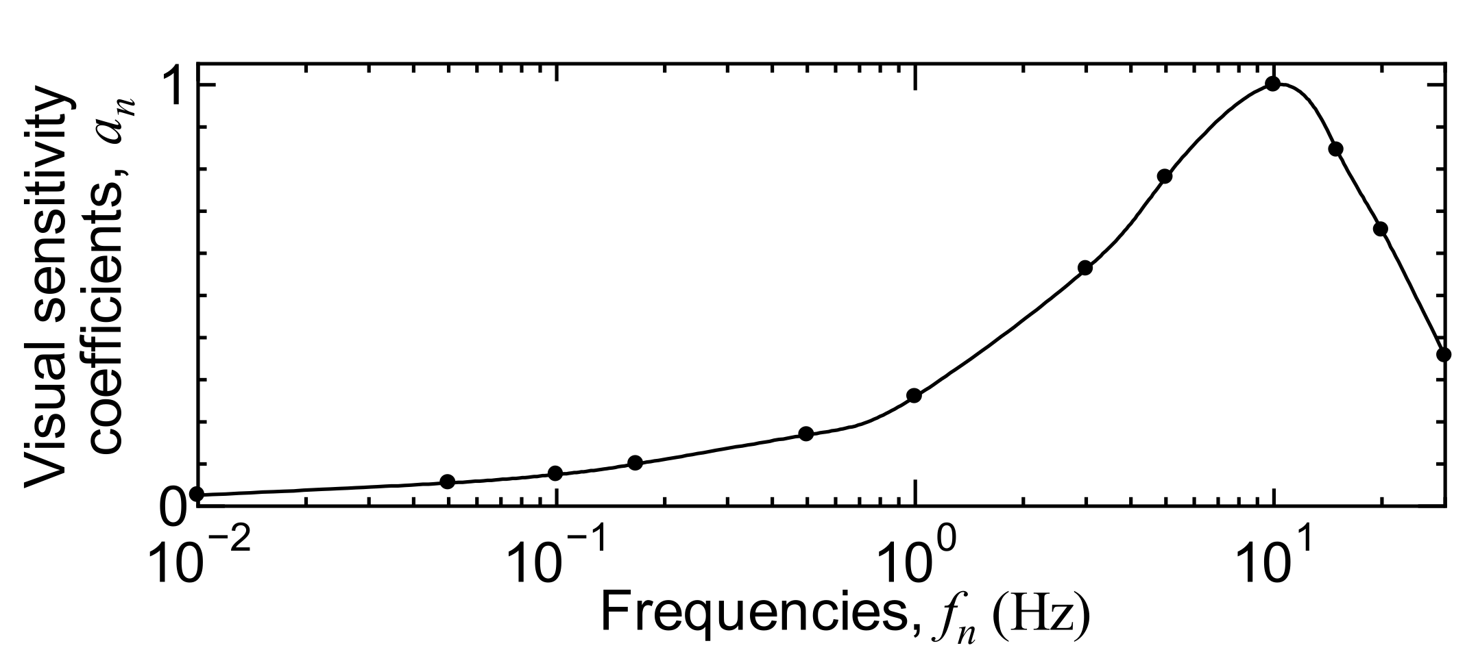
where $a_n$ is the visual sensitivity coefficient with $f_n$, as shown in Figure 1 [8] (p. 265). Figure 1 indicates that the $\Delta V_{10}$ algorithm is most sensitive to a 10 Hz voltage fluctuation. In a technical report published by The Institute of Electrical Engineers of Japan (IEEJ), it was proposed that the 4th highest $\Delta V_{10}$ out of 60 per hour (i.e., the 95th percentile) is considered as the maximum value [20], and the tolerable limit of the $\Delta V_{10}$ is set to 0.45 V [8] (p. 265).

Figure 1. Frequency dependence of visual sensitivity coefficients.

Voltage fluctuation, due to sources other than the output power variation of SWTs, is always present in the $V_{\mathrm{t}}$ that can be depicted by the fluctuation of the background voltage $\left(V_{\mathrm{u}}\right)$ in Equation (1). Thus, it is stated in many studies, including IEC61400-21 [21] (p. 32), that the flicker emission caused by WTs should not be directly measured using the $V_{\mathrm{t}}$ fluctuation at the WT terminal. Instead, it is specified that flicker emissions should be measured using the active and reactive power ($P$ and $Q$ in Equation (1)) [9], or current and voltage time-series [21] (p. 32) from the WTs. However, there are many restrictions to the specified methods. For instance, it is important to use a grid with minimal $V_{\mathrm{t}}$ fluctuation to certify the flicker emission from fixed-speed WTs with induction generators connected directly to the grid, as their active and reactive powers ($P$ and $Q$) are affected by $V_{\mathrm{t}}$ fluctuations [9]. In fact, the flicker emission evaluated from the total active and reactive power from all fixed-speed WTs in a wind park was much higher than the figure estimated from the flicker of one WT, using the formula from IEC61400-21 [21] (p. 137), and the most likely reason for this is a greater $V_{\mathrm{t}}$ fluctuation during the measurement obtained from all WTs [9]. In contrast, another study reported that the flicker emission evaluated from the total active and reactive powers from a wind power plant, comprised of variable-speed WTs with power electronic devices for partial power management (type III), was lower than the value estimated from the flicker of one WT using the same formula [22]. Thus, it is evident that more studies are needed to confirm these results. It has been noted that the specified method used to measure flicker emissions is not relevant to characterizing a WT with a voltage-controlling power converter [23].

The purpose of this study is not to evaluate flicker emissions from specific SWTs but to describe practical instances of flicker emissions from small wind power facilities, as such data are rarely published. Thus, in this study, flicker emissions were measured directly from the $V_{\mathrm{t}}$ fluctuation at the PCC using a flicker meter.

3. Small Wind Power Facility and Measurement Arrangement at the Site in Minami-Osumi

The small wind power facility monitored in this study is located at Nejime, a few kilometers away from the west coast of the Osumi Peninsula in Minami-Osumi, Kagoshima, Japan. The facility consists of two pitch-regulated 10 kW SWTs, WT-A, and WT-B. The specifications of the WTs are listed in Table 1.

Table 1. Specifications of the wind turbines monitored at the site in Minami-Osumi.

Model	ANE AH—10 kW
Rated power (at 11 m/s)	10 kW
Rotor diameter	7.8 m
Number of blades	3
Working wind speed	3–25 m/s
Rated rotor speed	180 rpm

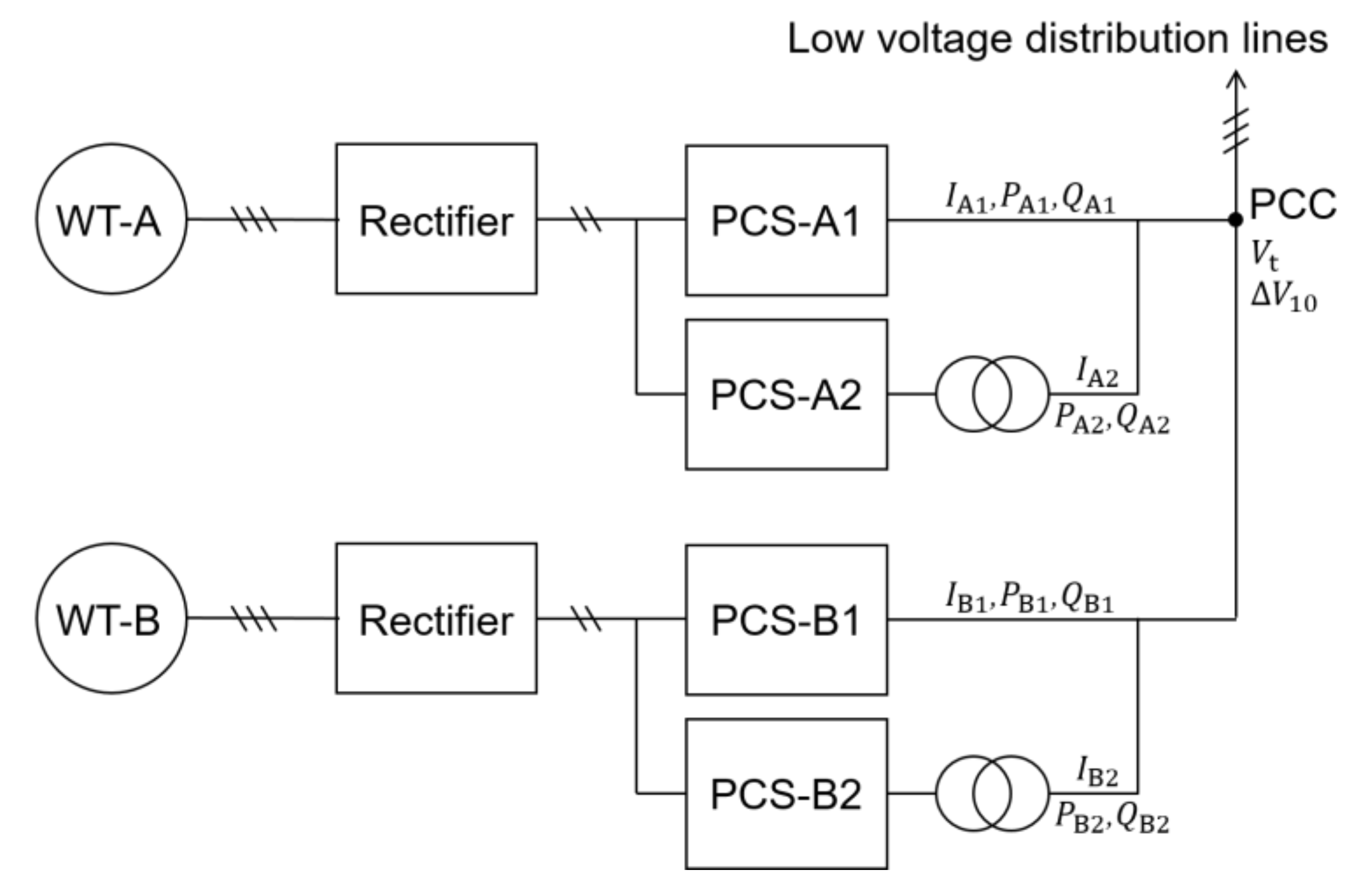
Figure 2 illustrates the main electrical circuit of the facility. In each SWT system, the alternating current (AC) output power from the generator is rectified into direct current (DC) power once, then input into two 5.0 kW power conditioning systems (PCSs), connected to 100/200 V single-phase three-wire distribution lines, and sent to the LV distribution lines. One of the PCSs in each SWT system is connected to the grid via an isolation transformer to prevent a short circuit of distribution lines through the DC lines. In this study, the PCC voltage $\left(V_{\mathrm{t}}\right)$ and equivalent 10 Hz flicker emission $(\Delta V_{10})$ at the PCC were monitored. Additionally, the output current and active and reactive power from respective PCSs were monitored. The voltage, current, and power were measured using clamp-on power meters (3169-01 by HIOKI, Nagano, Japan), which generated measurement data in analog (D/A) form updated every cycle (20 ms) with a delay of a few cycles. The flicker emission index $\left(\Delta V_{10}\right)$ was measured using a flicker meter (IFK-40 by Q-tecno, Fukuoka, Japan), which generated measurement data in analog (D/A) form updated every minute with a one-minute delay. The one-minute delay of the analog signal was inevitable in principle and compensated in the data shown, hereafter, in this paper.

Figure 2. Circuit configuration of the small wind power facility at the site in Minami-Osumi.

Furthermore, the wind speed and direction were monitored at the hub height (15 m) using an ultrasonic anemometer (WindObserver 65 by Gill, Lymington, UK), which generated measurement data in analog (D/A) form updated every 0.1 s. The layout of the anemometer and the two SWTs at the site are illustrated in Figure 3. When the meteorological wind direction is (6 $\pm$15)$°$ and (149$\pm$15)$°$, the wake effect of WT-A and WT-B may affect the measured values, respectively.

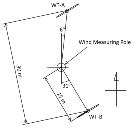
Figure 3. Layout of the site in Minami-Osumi.

All the analog signals from the instruments for measurement were recorded by a data logger (Yokogawa GP10) at an interval of 0.1 s. The measurement period was almost a year, from 11 September 2019 to 6 September 2020.

Figure 4a shows the wind rose drawn using the annual measurement data. Figure 4a indicates that the northwest was the predominant wind direction. The site was 217 m above sea level, and the terrain opened toward the mouth of the Ogawa River, 3.5 km away, in the same direction. Figure 4b shows the turbulence intensity in a minute. In Figure 4b, the data for the periods during which the wind direction remained above 5% per minute in the wake from any SWT were eliminated.

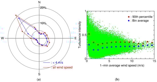
Figure 4. Wind characteristics at the site in Minami-Osumi. (a) Wind rose at site. (b) Turbulence intensity.

4. Evaluation of Flicker Emissions at the Site in Minami-Osumi

4.1. Thevenin Equivalent Resistance

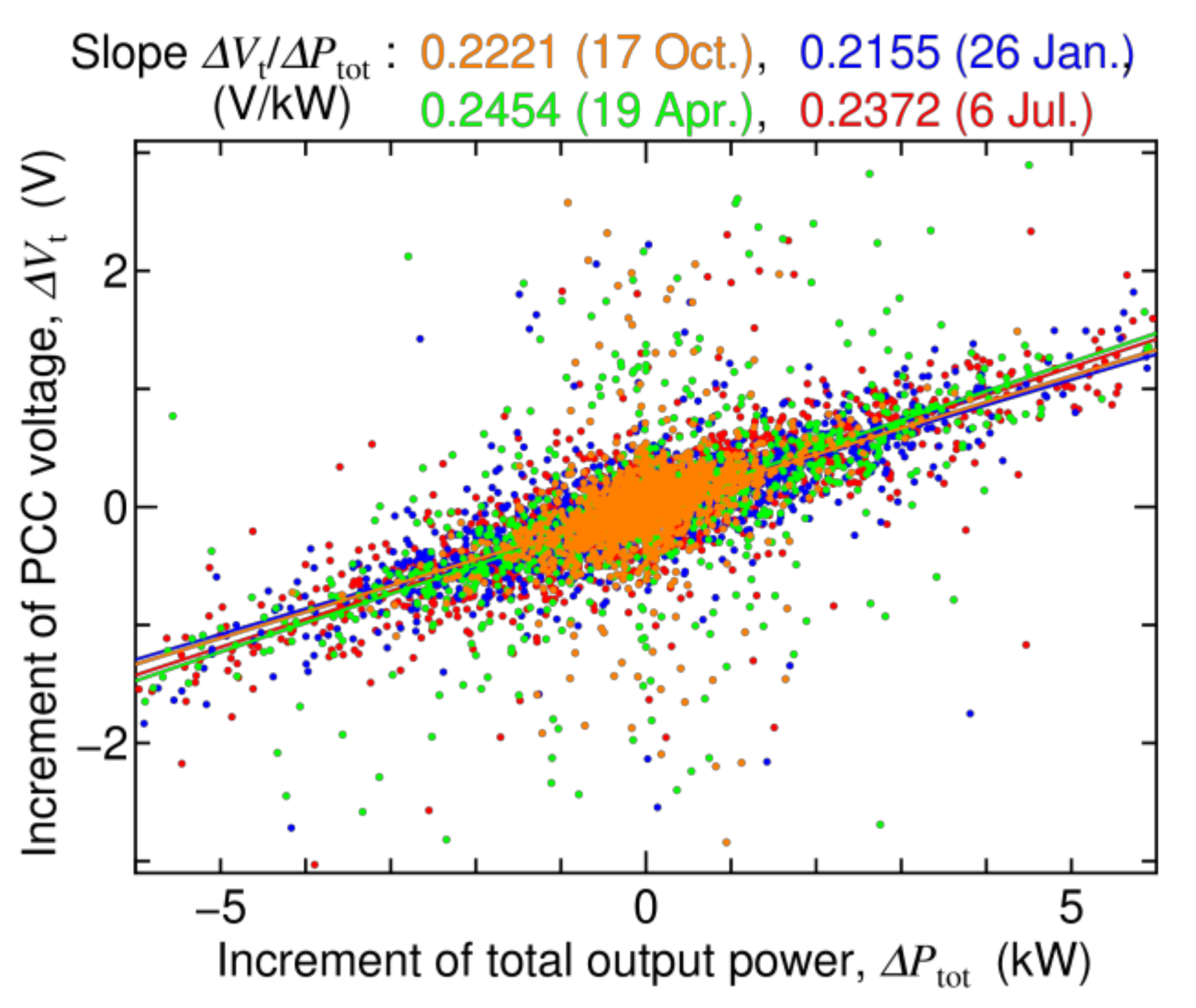
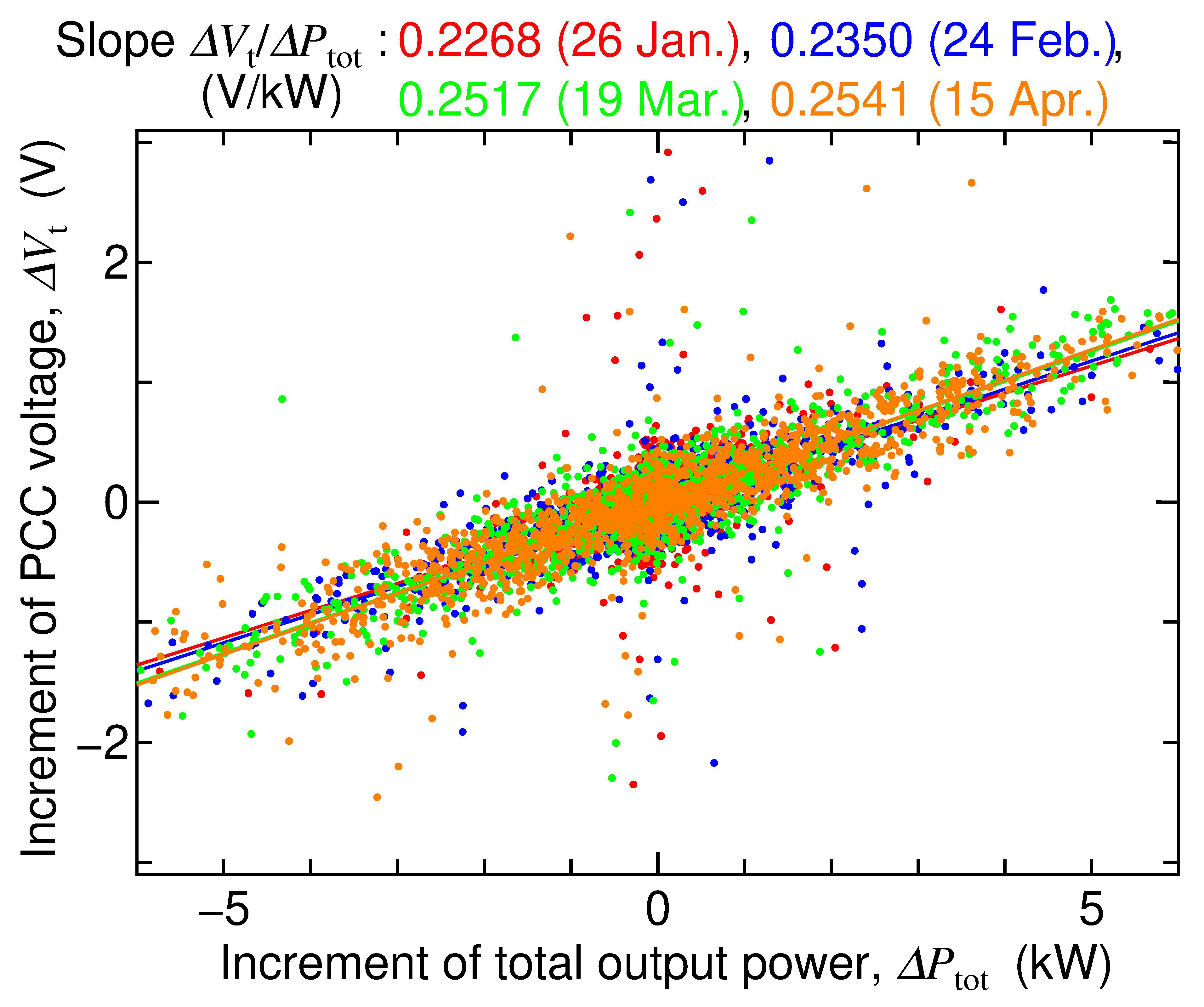
As mentioned in Section 2.1, the Thevenin equivalent resistance is a variable that directly affects voltage fluctuations at the PCC that are caused by the output power variations of the SWTs. Thus, it was evaluated using the time-series data of the PCC voltage $V_{\mathrm{t}}$ and total output power $P_{\mathrm{tot}} \left(=P_{\mathrm{A}1}+P_{\mathrm{A}2}+P_{\mathrm{B}1}+P_{\mathrm{B}2}\right)$. The relationship between the increments of the PCC voltage $\left(\Delta V_{\mathrm{t}}\right)$ and the total output power $(\Delta P_{\mathrm{tot}}),$ over a period of four days, is shown in Figure 5. If there is no factor that causes voltage fluctuations other than the SWTs and the PCSs operated with a power factor of one, theoretically, the points on each day in Figure 5 are arranged in a straight line and the slope $\Delta V_{\mathrm{t}}$/$\Delta P_{\mathrm{tot}}$ represents $R$/$V_{\mathrm{t}}$ as described in Equation (1). The increment processing is similar to the time-differentiating of the measured data and is conducted to eliminate the influence of long-term variations, such as tap-changing of substation transformers. The time-differentiating process was used to estimate the Thevenin equivalent impedance in an earlier study, and valid results were obtained [24].

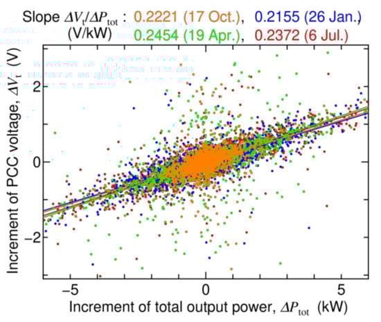
Figure 5. Relationship between increments of $V_{\mathrm{t}}$ and $P_{\mathrm{tot}}$ over four days at the site in Minami-Osumi.

The values of slopes $\Delta V_{\mathrm{t}}$/$\Delta P_{\mathrm{tot}}$ of the straight lines drawn using the least-squares method for the respective days had slight errors, and an average of 0.230 V/kW. In accordance with an approximation of the PCC voltage $V_{\mathrm{t}}$ to 200 V, the average slope corresponded to 0.0460 V/A as the line current for 1 kW was 5 A. Thus, the Thevenin equivalent resistance $(R$) per line was estimated to be 0.0230 Ω. Given that, in Japan, the line resistance value used in the certification tests on PCSs for small-scale dispersed power-generating systems is 0.190 Ω [25] (p. 13), it is considered that the voltage fluctuation at this site is almost one-eighth of the condition assumed in the certification tests. The reason for the low resistance is that the pole transformer that lowers the voltage from 6.6 kV to 100/200 V is placed close to the site, and the length of the LV distribution lines from the transformer is short.

4.2. Flicker Emission and Total Output Power

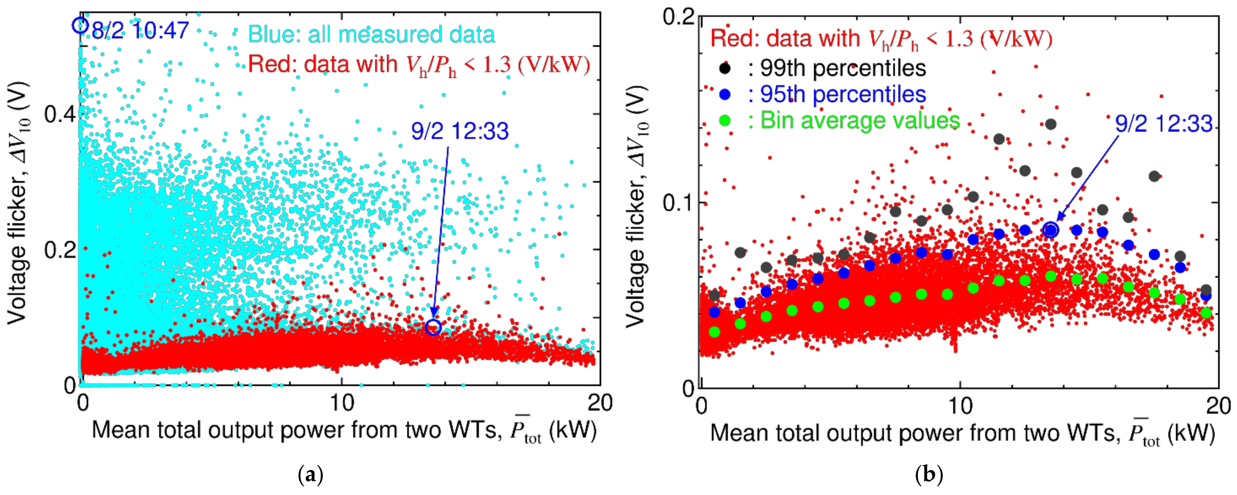
The raw data of the annual measurement of the relationship between the flicker emission index $\Delta V_{10}$ at the PCC and the mean total output power ${\overline{P}}_{\mathrm{tot}}$ are represented in a scatter plot by the blue and red dots in Figure 6a. Figure 6a indicates that the $\Delta V_{10}$ at the PCC was sometimes higher than the tolerable limit (0.45 V), even if ${\overline{P}}_{\mathrm{tot}}\cong 0$ kW. This means that the PCC voltage often fluctuated, not just as a result of the output power variation from the SWTs, but from other factors whose origin is unclear. Figure 6b is the scatter plot with valid flicker emission data only, where the method to extract the valid data is described later in Section 4.3.

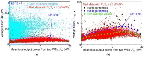
Figure 6. Scatter plot representing the relationship between the flicker emission $\Delta V_{10}$ and the mean total output power ${\overline{P}}_{\mathrm{tot}}$. (a) Measured data. (b) Extracted data.

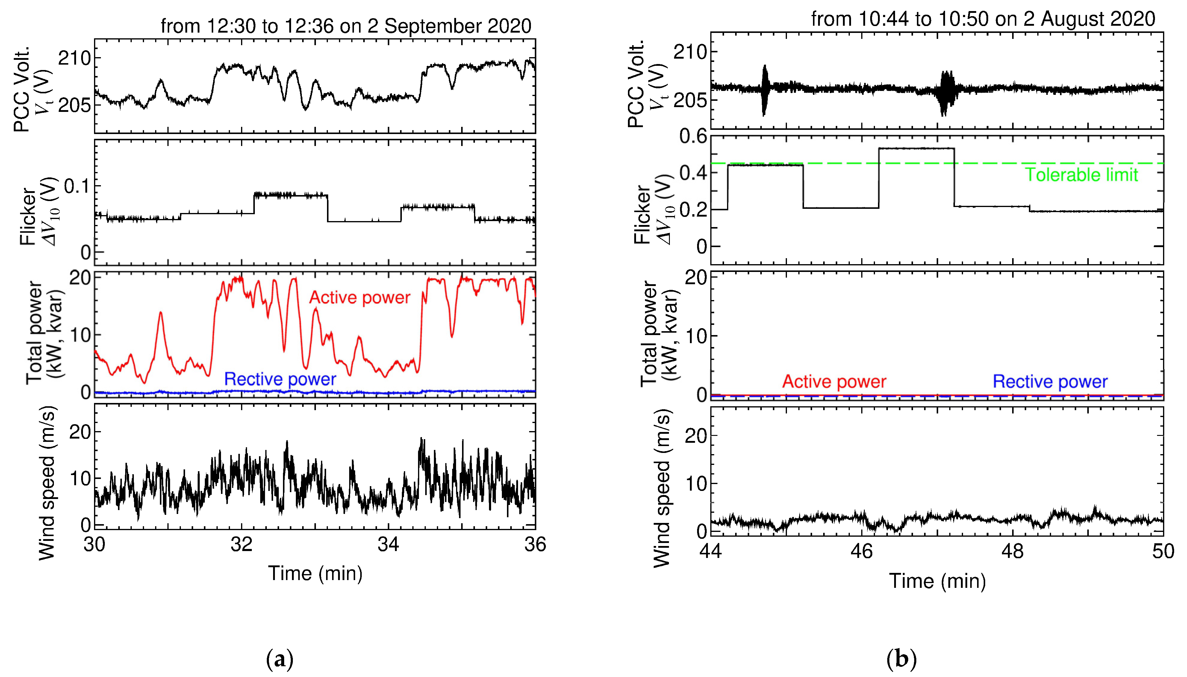
Two typical examples of time variation at the times highlighted in Figure 6a are shown in Figure 7. The first example (Figure 7a) is at 12:33 on 2 September with a mean wind speed of 9.4 m/s, ${\overline{P}}_{\mathrm{tot}}=13.5$ kW, and $\Delta V_{10}=0.085$ V, and the period a few minutes before and after. In this case, the total output active power $P_{\mathrm{tot}}$ fluctuated drastically according to the variation in wind speed, and the fluctuation of the PCC voltage $V_{\mathrm{t}}$ was synchronized with $P_{\mathrm{tot}}$ to some extent. In short, the fluctuation of the PCC voltage $V_{\mathrm{t}}$ was primarily caused by the fluctuation of $P_{\mathrm{tot}}$. The fluctuation component of the 200 V system voltage $V_{\mathrm{t}}$ with a frequency of $f_n\cong$ 0.07 Hz (a period of $~$15 s) and an amplitude of $\left(200/100\right)·\Delta v_n\cong$ 1.5 V is, roughly speaking, remarkable at 12:33. The flicker emission index $\Delta V_{10}^{*}$ derived from only the remarkable frequency component is calculated at 0.049 V using Equation (2) with $a_n\cong$0.065. The roughly calculated $\Delta V_{10}^{*}$ is 58% of the $\Delta V_{10}$ measured at 12:33, which is a major factor in the slightly high $\Delta V_{10}$ at the time.

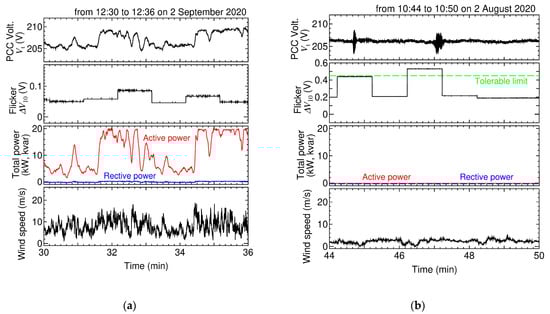
Figure 7. Two examples of time variation on the wind speed, total output power, PCC voltage, and flicker emission index. (a) At approximately 12:33 on 2 September 2020. (b) At approximately 10:47 on 2 August 2020.

The second example (Figure 7b) is at 10:47 on 2 August with a mean wind speed of 2.2 m/s, ${\overline{P}}_{\mathrm{tot}}=0$ kW, and $\Delta V_{10}=0.530$ V, and the period a few minutes before and after. In this case, the PCC voltage $V_{\mathrm{t}}$ had high-frequency components, which must therefore be the key factor in the higher $\Delta V_{10}$ than the tolerable limit at that time. Nevertheless, the wind speed was too low for SWTs to generate power. The severe PCC voltage fluctuation at the time was not from the SWTs but from other factors.

4.3. Power Spectra and Data Extraction

The power spectral density $(v_f)$ of the PCC voltage $V_{\mathrm{t}}$ and power spectral density $\left(p_f\right)$ of the total output active power $P_{\mathrm{tot}}$ for several minutes around 12:33 on 2 September in Figure 7a with the Hanning window are depicted in Figure 8. The ratio ${\overline{v}}_f/{\overline{p}}_f$ of their bin averages is depicted in Figure 8, too. The ratio ${\overline{v}}_f/{\overline{p}}_f$ of the low-frequency components is close to the average slope of 0.230 V/kW in Figure 5, which can be interpreted as the low-frequency variation of the $V_{\mathrm{t}}$ being primarily caused by the fluctuation of the $P_{\mathrm{tot}}$ according to Equation (1). In contrast, the ratio at the frequency $f\gtrsim$0.3 Hz is higher than 0.230 V/kW and reaches a maximum of ten times, which is caused by the following two reasons:

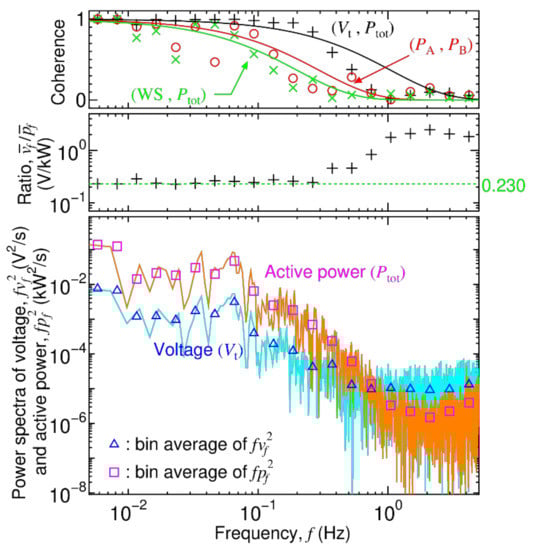
Figure 8. Power spectra of the PCC voltage $V_{\mathrm{t}}$ and total output active power $P_{\mathrm{tot}}$, their ratio, and coherence for the period in Figure 7a.

• Voltage variation largely caused not by the SWTs but other factors, as in the case of Figure 7b.
• Errors in the time-series data. In particular, the signal-to-noise ratio of the $V_{\mathrm{t}}$ data is lower than that of the $P_{\mathrm{tot}}$ data, because the variation in the $V_{\mathrm{t}}$ is only $\sim$1% (a few volts over a nominal voltage of 200 V).

The first factor presents itself only when other factors materialize, although the second is thought to be common for all measurement periods. Then, the superimposed effect of these two factors results in an increase in the ratios of the high-frequency components. Thus, valid $\Delta V_{10}$ data are extracted from all measured data in Figure 6a while focusing on the ratio. In particular, $\Delta V_{10}$ data measured in periods when $V_{\mathrm{h}}/P_{\mathrm{h}}$ is lower than a threshold value are considered valid, where $V_{\mathrm{h}}$ and $P_{\mathrm{h}}$ are defined in Equation (3):

$$V_{\mathrm{h}}=\sqrt{{{\displaystyle \sum }}_{f\ge 0.5\mathrm{Hz}}{v}_f^2},P_{\mathrm{h}}=\sqrt{{{\displaystyle \sum }}_{f\ge 0.5\mathrm{Hz}}{p}_f^2}$$

(3)

The scatter plot of $\Delta V_{10}$ and ${\overline{P}}_{\mathrm{tot}}$ with only the extracted data is shown in Figure 6b with the average, 95th, and 99th percentiles of $\Delta V_{10}$ for each ${\overline{P}}_{\mathrm{tot}}$ bin. The threshold value for the extraction was set to 1.3 V/kW while focusing on the appearance of clear characteristics on the 95th percentiles of the $\Delta V_{10}$, which is the most important to evaluate the flicker emission, and the rate of extracted data was 9.7% of all the data under the power-generating condition. This extraction methodology is not available if the PCC voltage fluctuation caused not by the SWTs but other factors is always high.

4.4. Analysis of Flicker Emissions from SWTs

The irregular distribution of the 99th percentiles in Figure 6b indicates that some data that should be eliminated are still included in the extracted data. However, the bin averages and 95th percentiles of the $\Delta V_{10}$ distribution change smoothly, depending on the mean total output power ${\overline{P}}_{\mathrm{tot}}$ with the peak at ${\overline{P}}_{\mathrm{tot}}=13~14$ kW (2/3 of the total power rating). When the 95th percentiles are focused according to the proposal by IEEJ, as described in Section 2.2, the peak value of 0.085 V is significantly lower than the tolerable limit of 0.45 V.

Although the data at the periods when the high-frequency variation of the PCC voltage $V_{\mathrm{t}}$ is not caused principally by SWTs have been removed in Figure 6b, the flicker emission in the extracted data is derived from both SWTs and other factors. When there is no correlation between the $V_{\mathrm{t}}$ variation by SWTs and by the other factors, the $\Delta V_{10}$ is represented using the following Equation [8] (p. 265):

$$\Delta V_{10}=\sqrt{{\left(\Delta V_{10}^{\mathrm{SWTs}}\right)}^2+{\left(\Delta V_{10}^{\mathrm{OF}}\right)}^2},$$

(4)

where $\Delta V_{10}^{\mathrm{SWTs}}$ and $\Delta V_{10}^{\mathrm{OF}}$ are $\Delta V_{10}$ solely caused by the two SWTs and other factors, respectively. If the 95th percentile of the $\Delta V_{10}$ at ${\overline{P}}_{\mathrm{tot}}=0~1$ kW was substituted for $\Delta V_{10}^{\mathrm{OF}}$, $\Delta V_{10}^{\mathrm{SWTs}}$ was estimated to be ${\left({0.085}^2-{0.041}^2\right)}^{1/2}=0.074$ V. According to Equation (5) in IEC61400-21 [21] (p. 137), the relationship between the flicker emissions by $N$ SWTs $\Delta V_{10}^{\mathrm{SWTs}}$ and a single SWT $\Delta V_{10}^{\mathrm{aSWT}}$ is

$$\Delta V_{10}^{\mathrm{SWTs}}=\sqrt{N}·\Delta V_{10}^{\mathrm{aSWT}},$$

(5)

based on the assumption that the output power variations of the SWTs have little correlation with each other, on the high-frequency components with high visual sensitivity coefficients $a_n$. The flicker emission $\Delta V_{10}^{\mathrm{aSWT}}$ by the single 10 kW SWT was estimated to be 0.053 V at the site. Even if the total power rating at the site is increased to 50 kW, which is the maximum capacity to be connected with low-voltage distribution systems in Japan, $\Delta V_{10}^{\mathrm{SWTs}}$ is estimated to increase to 0.117 V, that is lower than the tolerable limit (0.45 V).

4.5. Coherence

Coherence is an indicator of the frequency characteristics of correlation and is used to analyze the smoothing effects at wind farms [26]. The specific calculation method for coherence is explained in detail in a report [27] for a project launched by the authors of [26].

The coherence of the output power from WT-A $P_{\mathrm{A}} \left(=P_{\mathrm{A}1}+P_{\mathrm{A}2}\right)$ and WT-B $P_{\mathrm{B}} \left(=P_{\mathrm{B}1}+P_{\mathrm{B}2}\right)$ is depicted with circles (○) in Figure 8. The solid curve in red is the Davenport-type decay curve exp $\left(-\alpha f\right)$ obtained by fitting the coherence values depicted with the circles, in which the inverse of the decay coefficient, $1/\alpha$, is 0.30 Hz. Even though this type of curve was used for the detailed investigation performed in [26], the coherence at this site decreased more rapidly with an increasing frequency, compared to the decay curve. The coherence was close to zero on the high-frequency components with $f\gtrsim$ 0.2 Hz, which means that the output power variations of the SWTs had little correlation to each other. This characteristic partially supports the explanation in Section 4.4. However, the coherence is close to one at $f\cong$0.07 Hz, which is the frequency of a main component on the $V_{\mathrm{t}}$ variation, at the time, in Figure 7a. This means that the output power variation of the two SWTs is almost synchronized to the frequency component. Thus, the flicker emission index $\Delta V_{10}^{\mathrm{SWTs}}$ by multiple SWTs should be estimated not by Equation (5), but the following Equation (6) when such a low-frequency component is dominant:

$$\Delta V_{10}^{\mathrm{SWTs}}=N·\Delta V_{10}^{\mathrm{aSWT}},$$

(6)

By Equation (6), the flicker emission $\Delta V_{10}^{\mathrm{aSWT}}$ by the single 10 kW SWT was estimated to be 0.037 V at the site. Even if the total power rating was increased until 50 kW at the site, $\Delta V_{10}^{\mathrm{SWTs}}$ was estimated to increase until 0.185 V that is lower than the tolerable limit (0.45 V).

Next, the coherence between the total output power $P_{\mathrm{tot}}$ and PCC voltage $V_{\mathrm{t}}$ is shown with $+$ shapes in Figure 8. The solid curve in black is the Davenport-type decay curve obtained by fitting the coherence values shown with $+$ shapes, whereby the inverse of the decay coefficient, $1/\alpha$, is 1.05 Hz. The coherence is close to one on the low-frequency components with $f\lesssim$0.3 Hz, which means that the low-frequency variation of the PCC voltage $V_{\mathrm{t}}$ is derived from the total output power $P_{\mathrm{tot}}$, and then it decreases with the increase in the frequency $f$. This characteristic supports the explanation presented in Section 4.3.

Finally, the coherence between the total output power $P_{\mathrm{tot}}$ and wind speed is shown with $\times$ shapes in Figure 8. The solid curve in green is the Davenport-type decay curve obtained by fitting the coherence values shown with $\times$ shapes, whereby the inverse of the decay coefficient, $1/\alpha$, is 0.20 Hz. The coherence is close to one on the low-frequency components with $f\lesssim$0.07 Hz, with a few exceptions, which is consistent with the principle that fluctuations in the output of wind power generation are caused by fluctuations in the wind speed. Furthermore, the time variation of the $P_{\mathrm{tot}}$ appears smoother than that of the wind speed in Figure 7a. The reason for this is that, in variable-speed WTs, the variation in short-term mechanical input power is absorbed as the variation of the kinetic energy in the turbine rotor, owing to the slight change in rotational speed, as described in Section 1. Hence, the coherence is close to zero for high-frequency components.

4.6. Turbulence Intensity

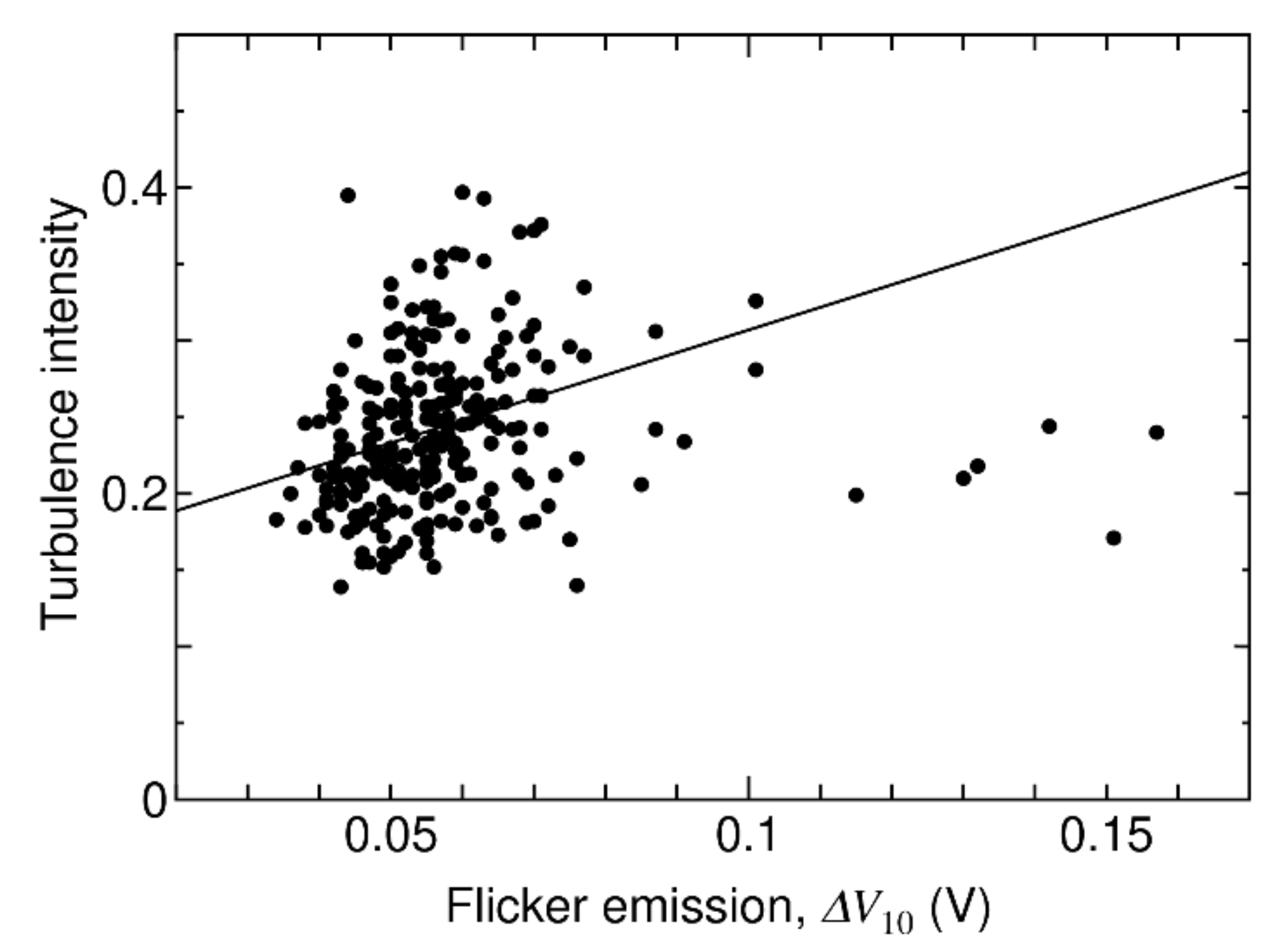
Wind speed variation causes the fluctuation of the total output active power $P_{\mathrm{tot}}$ as described in Section 4.2, and then the $P_{\mathrm{tot}}$ fluctuation causes the fluctuation of the PCC voltage $V_{\mathrm{t}},$ as expressed in Equation (1). $\Delta V_{10}$ is an index related to the variation in PCC voltage $V_{\mathrm{t}}$. In contrast, turbulence intensity is another index used to represent the wind speed variation in wind turbine design and classification. Thus, the relationship between the turbulence intensity and $\Delta V_{10}$ was investigated. Figure 9 shows the relationship between the turbulence intensity and flicker emission index $\Delta V_{10}$ in the periods with ${\overline{P}}_{\mathrm{tot}}=13~14$ kW as a scatter plot. The data for the periods during which the wind direction stayed above 5% per minute in the wake from any SWT were eliminated.

Figure 9. Relationship between turbulence intensity and flicker emission index $\Delta V_{10}$ in the periods with ${\overline{P}}_{\mathrm{tot}}=13~14$ kW.

In Figure 9, a straight line is drawn using the least-squares method while eliminating the data with $\Delta V_{10}\ge 0.09$ V. The data with high $\Delta V_{10}$ were eliminated because such data seem to be affected by the high-frequency voltage fluctuation, to some extent, and as a result of other factors, rather than the SWTs. Although the line represents the positive correlation between the turbulence intensity and the $\Delta V_{10}$, the data are, rather, distributed on the graph. The possible reasons for this are the variation in voltage as a result of other factors, and the fact that $\Delta V_{10}$ is highly influenced by the change rate of the voltage as weighted by the visual sensitivity coefficients $a_n$, unlike the turbulence intensity that is an index that loses information of the change rate of the wind speed.

5. Re-Evaluation of the Results from the Site in Wakkanai

Although the authors have already reported the measurement results from another site in Wakkanai in [17], they re-evaluated the same results in this section to compare them with the results obtained from the Minami-Osumi site described in Section 4. The following improved methods were used in this study for the re-evaluation process:

• Increments were used for the estimation of the Thevenin equivalent resistance, as described in Section 4.1.
• Valid $\Delta V_{10}$ data were extracted while focusing on the ratio $V_{\mathrm{h}}/P_{\mathrm{h}},$ as described in Section 4.3.

The small wind power facility was located at Tomioka, approximately 400 m away from the north coast and facing Soya Bay in Wakkanai, Hokkaido, Japan. The facility consisted of four pitch-regulated 4.9 kW SWTs, named WT-1 to WT-4. The distance between WT-2 and WT-3 was 27 m, which was almost the same distance between WT-A and WT-B at the site in Minami-Osumi. However, the other distances exceeded 43 m. The specifications of the WTs are listed in Table 2.

Table 2. Specification of wind turbines monitored at the site in Wakkanai.

Model	Zephyr 9000
Rated power (continuous max)	4.9 kW
Rotor diameter	5.5 m
Number of blades	3
Cut-in wind speed	3.5 m/s
Rated rotor speed	277 rpm

Figure 10 illustrates the main electrical circuitry of the facility. In each SWT system, the AC output power from the generator is rectified into DC power once, then input into a 5.8 kW PCS connected to 100/200 V single-phase three-wire distribution lines, and sent to the LV distribution lines. The AC side measurement was conducted in a similar way, using the same instruments as those used for the measurement conducted at the Minami-Osumi site. Specifically, the PCC voltage $V_{\mathrm{t}}$, output current, and active and reactive power from respective PCSs were measured using clamp-on power meters (HIOKI 3169-01), and the flicker emission index $\Delta V_{10}$ was measured using a flicker meter (Q-tecno IFK-40).

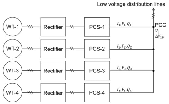
Figure 10. Circuit configuration of the small wind power facility at the site in Wakkanai.

Although the wind speed and direction were monitored by the same ultrasonic anemometer (Gill WindObserver 65) used at the site in Minami-Osumi, the measurement location was more than 100 m apart from the SWTs, and 8 m above the ground, which was lower than the hub height (12.1 m). Thus, the wind data are only taken as a reference in this study.

The measurement period was approximately 4 months, from 20 December 2017 to 24 April 2018.

5.1. Thevenin Equivalent Resistance

Comparable with the process from Section 4.1 for the site in Minami-Osumi, the Thevenin equivalent resistance at the site in Wakkanai was evaluated using the time-series data of the PCC voltage $V_{\mathrm{t}}$ and the total output power $P_{\mathrm{tot}} \left(=P_1+P_2+P_3+P_4\right)$. The relationship between the increments of the PCC voltage $\Delta V_{\mathrm{t}}$ and the total output power $\Delta P_{\mathrm{tot}}$ over four days is illustrated in Figure 11. The dispersion of the data is much smaller than the scatter plot of the relationship between $V_{\mathrm{t}}$ and $P_{\mathrm{tot}}$ depicted in a previous report [17]. The values of slopes $\Delta V_{\mathrm{t}}$/$\Delta P_{\mathrm{tot}}$ of the straight lines drawn by the least-squares method for the respective days have slight errors, with an average of 0.242 V/kW. Under a rough approximation of the PCC voltage $V_{\mathrm{t}}$ to 200 V, the average slope corresponds to 0.0460 V/A. Thus, the Thevenin equivalent resistance $R$ per line was estimated to be 0.0242 Ω. The resistance is almost the same as that obtained at the site in Minami-Osumi, and the reason for the low resistance is that the pole transformer was placed close to the site.

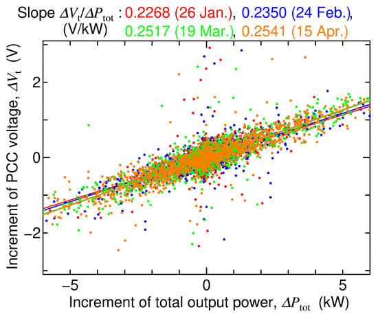
Figure 11. Relationship between increments of $V_{\mathrm{t}}$ and $P_{\mathrm{tot}}$ over four days at the site in Wakkanai.

5.2. Flicker Emission and Total Output Power

The raw data of the four-month measurement of the relationship between the flicker emission index $\Delta V_{10}$ at the PCC and the mean total output power ${\overline{P}}_{\mathrm{tot}}$ are shown in a scatter plot by blue and red dots in Figure 12a. Figure 12a indicates that the $\Delta V_{10}$ at the PCC was rather calm and always lower than the tolerable limit (0.45 V). Thus, in a previous report [17], the flicker emission was evaluated using the raw data. In contrast, in this study, the data in Figure 12b were extracted in terms of the $V_{\mathrm{h}}/P_{\mathrm{h}}$ threshold of 1.3 V/kW as described in Section 4.3, and the rate of extracted data was 87.1% of all the data under the power-generating condition, which is a much higher rate than at the site in Minami-Osumi. As both the total power rating and the Thevenin equivalent resistance at the site in Minami-Osumi are almost the same, which means that the impact of the SWT output power fluctuation on the voltage at the PCC is, theoretically, almost the same, the same threshold value is used for this site.

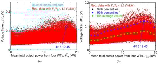
Figure 12. Scatter plot illustrating the relationship between the flicker emission $\Delta V_{10}$ and the mean total output power ${\overline{P}}_{\mathrm{tot}}$. (a) Measured data. (b) Extracted data.

In Figure 12b, all of the bin averages and 95th and 99th percentiles of the $\Delta V_{10}$ distribution change smoothly, depending on the mean total output power ${\overline{P}}_{\mathrm{tot}}$, with the peak at ${\overline{P}}_{\mathrm{tot}}=16~17$ kW (5/6 of the total power rating). The peak value of the 95th percentile is 0.122 V at 12:45 on 15 April, which is 0.04 V lower than that evaluated in the previous report [17], owing to the extraction treatment. The peak value is 1.4 times higher than that at the site in Minami-Osumi.

As analyzed in Section 4.4, flicker emissions solely caused by the four SWTs, $\Delta V_{10}^{\mathrm{SWTs}}$, are calculated as follows, using Equation (4): if the 95th percentile of the $\Delta V_{10}$ at ${\overline{P}}_{\mathrm{tot}}=0~1$ kW is substituted for $\Delta V_{10}^{\mathrm{OF}}$, then $\Delta V_{10}^{\mathrm{SWTs}}$ is estimated to be ${\left({0.122}^2-{0.063}^2\right)}^{1/2}=0.104$ V. It is also 1.4 times higher than that at the site in Minami-Osumi.

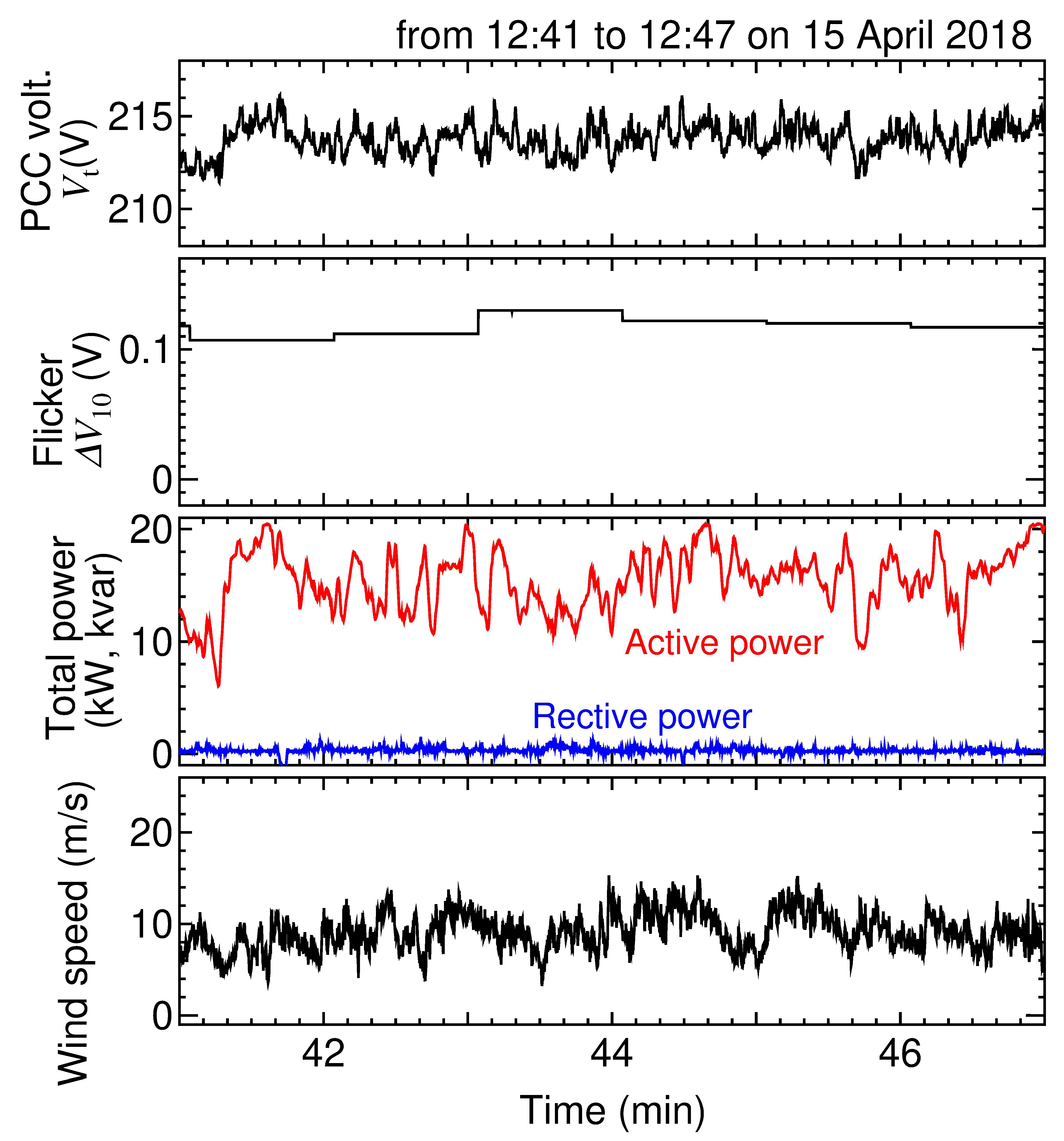
The time variation around 12:45 on 15 April with a mean wind speed of 9.9 m/s, ${\overline{P}}_{\mathrm{tot}}=16.9$ kW and $\Delta V_{10}=0.122$ V, the peak value of the 95th percentiles, and the period of a few minutes before and after is shown in Figure 13. Compared with Figure 7a, measured at the site in Minami-Osumi, the variation widths of the total output power $P_{\mathrm{tot}}$ and, consequently, the PCC voltage $V_{\mathrm{t}}$ were narrower, but the frequency was higher. The higher flicker emission $\Delta V_{10}$ was derived from the higher visual sensitivity coefficients $a_n$ due to the higher frequency components. The fluctuation component of the 200 V system voltage $V_{\mathrm{t}}$ with a frequency of $f_n\cong$0.15 Hz (a period of $~7$ s) and an amplitude of $\left(200/100\right)·\Delta v_n\cong$1.0 V is, roughly speaking, remarkable at 12:45. The flicker emission index $\Delta V_{10}^{*}$, derived only by the remarkable frequency component, is calculated as 0.05 V from Equation (2) with $a_n\cong$0.10. The roughly calculated $\Delta V_{10}^{*}$ is 41% of the $\Delta V_{10}$ measured at 12:45, which is one of the major factors in the slightly high $\Delta V_{10}$ at the time.

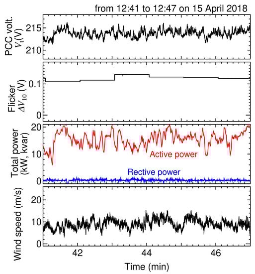
Figure 13. Time variation on the wind speed, total output power, PCC voltage, and flicker emission index at around 12:45 on 15 April 2018.

5.3. Power Spectra

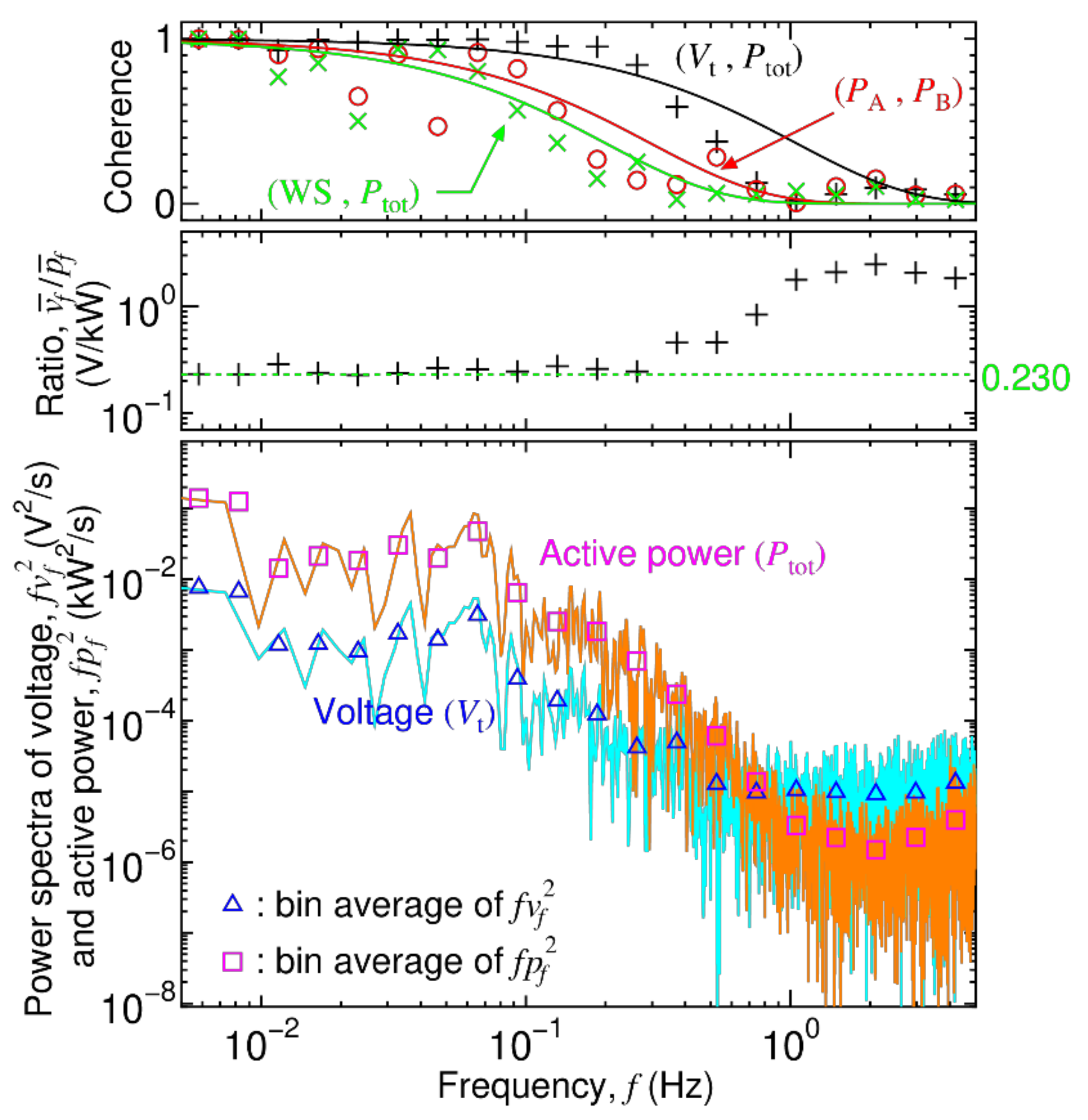
The power spectral density $v_f$ of the PCC voltage $V_{\mathrm{t}}$ and power spectral density $p_f$ of the total output active power $P_{\mathrm{tot}}$ for several minutes around 12:45 on 15 April (in Figure 13) with the Hanning window are depicted in Figure 14. Compared with Figure 8 measured at the site in Minami-Osumi, the amplitudes of the high-frequency components with $f\gtrsim$ 0.1 Hz are higher in the total output power $P_{\mathrm{tot}}$ and, therefore, the PCC voltage $V_{\mathrm{t}}$, although those on the low-frequency components with $f\lesssim$ 0.1 Hz are vice versa. This $V_{\mathrm{t}}$ feature supports the explanation with regards to the impact of the 0.15 Hz component on the slightly high $\Delta V_{10}$ in Section 5.2, and also demonstrates the influence of the higher components with higher visual sensitivity coefficients $a_n$.

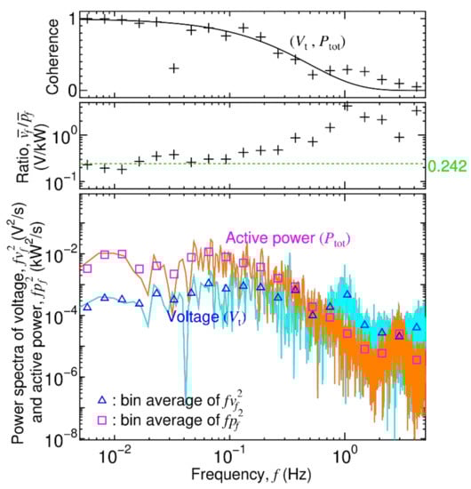
Figure 14. Power spectra of the PCC voltage $V_{\mathrm{t}}$ and the total output active power $P_{\mathrm{tot}}$, their ratio, and coherence for the period in Figure 13.

The ratio ${\overline{v}}_f/{\overline{p}}_f$ of the bin averages is shown in Figure 14. The ratio ${\overline{v}}_f/{\overline{p}}_f$ of the low-frequency components is close to the average slope of 0.242 V/kW in Figure 11, which can be interpreted as the low-frequency variation of the $V_{\mathrm{t}}$ being primarily caused by the fluctuation of the $P_{\mathrm{tot}}$ according to Equation (1). Conversely, the ratio at the frequency of $f\gtrsim$0.2 Hz is higher than 0.242 V/kW and reaches a maximum of eighteen times, which is caused by the two reasons described in Section 4.3.

5.4. Comparison of Flicker Emission

The flicker emission $\Delta V_{10}$ at the site in Wakkanai was evaluated to be 1.4 times higher than that at the site in Minami-Osumi, and the flicker emission $\Delta V_{10}^{\mathrm{SWTs}},$ solely caused by the SWTs, was also estimated to be 1.4 times higher than that at the site in Minami-Osumi, as described in Section 5.2. The higher flicker emission is derived from the higher amplitudes of the high-frequency components with $f\gtrsim$ 0.1 Hz in the total output power $P_{\mathrm{tot}}$ and thereby the PCC voltage $V_{\mathrm{t}}$, as is described in Section 5.3. The distances between the SWTs are greater, as described in Section 5.1, and there are twice the number of SWTs at the site in Wakkanai. Thus, the smoothing effect of output power fluctuations from multiple SWTs should be greater. Nevertheless, the high-frequency components were larger in the total output power $P_{\mathrm{tot}}$, signifying that the high-frequency components of a single SWT are larger at the site in Wakkanai. This could be due to the fact that the smaller-scale SWT has a smaller inertia constant of the rotational parts, such as a wind turbine rotor and a generator rotor [10]. That is, the effect of smoothing the output power fluctuation in each variable-speed WT against the mechanical input fluctuation caused by the wind speed variation, as described in Section 4.5, is weaker, owing to the lower level of inertia.

Next, the influence of the mean total output power ${\overline{P}}_{\mathrm{tot}}$ on the flicker emission $\Delta V_{10}$ is discussed. When ${\overline{P}}_{\mathrm{tot}}$ is close to zero, $P_{\mathrm{tot}}$ variation is generally small, and, consequently, $\Delta V_{10}$ is low. In contrast, when ${\overline{P}}_{\mathrm{tot}}$ is close to the total power rating, the blade pitch angles of the respective SWTs are generally controlled to maintain the output power to the rated ones; therefore, the $P_{\mathrm{tot}}$ variation is small and, consequently, $\Delta V_{10}$ is low. Thus, $\Delta V_{10}$ is high in any intermediate ${\overline{P}}_{\mathrm{tot}}$ state. From Figure 6b and Figure 12b, the ${\overline{P}}_{\mathrm{tot}}$ that maximizes the 95th percentile $\Delta V_{10}$ is 2/3 of the total power rating at the site in Minami-Osumi and 5/6 of that in Wakkanai, respectively. From the measurement results obtained from the two sites, it can be concluded that the flicker emission is the highest when the mean total output power is approximately 3/4 of the total power rating of small wind power facilities.

6. Conclusions

The flicker emissions from small wind power facilities were investigated based on the voltage flicker index $\Delta V_{10}$ at two sites in Japan, and the following results were obtained:

• The flicker emission solely caused by variable-speed SWTs with a total power rating of $\sim$20 kW was significantly lower than the upper limit at the two sites. Even if the total power rating was increased until 50 kW, which is the maximum capacity to be connected with low-voltage distribution systems in Japan, it was estimated that the flicker emission was lower than the tolerable limit. One reason for this is that the Thevenin equivalent resistance of the grids was as low as 0.023 Ω. Another reason may be that the inertia of the rotational parts, such as the wind turbine rotor and generator rotor, created a smoother output power fluctuation against the mechanical input fluctuations caused by the wind speed variation.
• The flicker emission was at its highest when the mean total output power was approximately 3/4 of the total power rating of small wind power facilities.
• It was beneficial to use the ratio of high-frequency components in the PCC voltage and total output power to extract valid flicker emission data from all the measured data, though this methodology was not available if the PCC voltage fluctuation caused not by the SWTs but other factors was always high.

The first result effectively shows that SWTs do not cause severe voltage variations and flicker emissions when the Thevenin equivalent resistance is similar to the two sites. As the flicker emission caused by the SWTs increases in proportion with the resistance, theoretically, attention should be payed when the distribution lines are long. The second result clarifies the mean total output power that should be focused on in terms of flicker emission. The third result presents a methodology to evaluate flicker emissions solely caused by SWTs when the raw data of the flicker meter is often affected by voltage fluctuations as a result of to other factors.

References

- Li, Y.; Gao, W.; Ruan, Y. Quantifying variabilities and impacts of massive photovoltaic integration in public power systems with PHS based on real measured data of Kyushu, Japan. Energy Procedia 2018, 152, 883–888. [Google Scholar] [CrossRef]
- International Electrotechnical Commission (IEC). Wind Turbines—Part 2: Small Wind Turbines, 3rd ed.; IEC 61400-2; IEC: Geneva, Switzerland, 2013. [Google Scholar]
- Agency for Natural Resources and Energy. FIT Information Disclosure Website. Available online: https://www.fit-portal.go.jp/PublicInfoSummary (accessed on 10 June 2021). (In Japanese).
- Matsuda, K.; Wada, M.; Furukawa, T.; Watanabe, M.; Takahashi, R. Measurement results for evaluation of impact on power system by small wind turbines. In Proceedings of the 2007 Tohoku Section Joint Convention of Institutes of Electrical and Information Engineers, Aomori, Japan, 23–24 August 2007; 2B22; p. 82. (In Japanese). [Google Scholar]
- Chalise, S.; Atia, H.R.; Poudel, B.; Tonkoski, R. Impact of Active Power Curtailment of Wind Turbines Connected to Residential Feeders for Overvoltage Prevention. IEEE Trans. Sustain. Energy 2015, 7, 471–479. [Google Scholar] [CrossRef]
- Larsson, A. Flicker emission of wind turbines during continuous operation. IEEE Trans. Energy Convers. 2002, 17, 114–118. [Google Scholar] [CrossRef]
- Larsson, Å.; Sørensen, P.; Santjer, F. Grid Impact of Variable-Speed Wind Turbines. In Proceedings of the European Wind Energy Conference (EWEC), Nice, France, 1–5 March 1999; pp. 786–789. [Google Scholar]
- The Japan Electric Association. Grid-Interconnection Code. In JEAC 9701-2019; The Japan Electric Association: Tokyo, Japan, 2019. (In Japanese) [Google Scholar]
- Thiringer, T.; Petru, T.; Lundberg, S. Flicker Contribution From Wind Turbine Installations. IEEE Trans. Energy Convers. 2004, 19, 157–163. [Google Scholar] [CrossRef]
- Kondoh, J.; Mizuno, H.; Funamoto, T. Fault Ride-Through Characteristics of Small Wind Turbines. Energies 2019, 12, 4587. [Google Scholar] [CrossRef] [Green Version]
- Liu, Y.J.; Chen, Y.C.; Lan, P.H.; Chang, T.P. Power Quality Measurements of a Horizontal Axial Small Wind Turbine. Appl. Mech. Mater. 2017, 870, 329–334. [Google Scholar] [CrossRef]
- Liu, Y.-J.; Lan, P.-H. Power Quality Assessments of a Commercial Grid-Connected Small Wind Turbine Product. In Proceedings of the 2016 IEEE 5th Global Conference on Consumer Electronics, Kyoto, Japan, 11–14 October 2016; pp. 1–4. [Google Scholar] [CrossRef]
- Mohammadi, E.; Fadaeinedjad, R.; Naji, H.R. Flicker emission, voltage fluctuations, and mechanical loads for small-scale stall- and yaw-controlled wind turbines. Energy Convers. Manag. 2018, 165, 567–577. [Google Scholar] [CrossRef]
- Long, C.; Farrag, M.E.A.; Zhou, C.; Hepburn, D.M. Statistical Quantification of Voltage Violations in Distribution Networks Penetrated by Small Wind Turbines and Battery Electric Vehicles. IEEE Trans. Power Syst. 2013, 28, 2403–2411. [Google Scholar] [CrossRef]
- Ani, S.O.; Polinder, H.; Ferreira, J.A. Comparison of Energy Yield of Small Wind Turbines in Low Wind Speed Areas. IEEE Trans. Sustain. Energy 2012, 4, 42–49. [Google Scholar] [CrossRef]
- Pagnini, L.C.; Burlando, M.; Repetto, M.P. Experimental power curve of small-size wind turbines in turbulent urban environment. Appl. Energy 2015, 154, 112–121. [Google Scholar] [CrossRef]
- Kashiwaya, K.; Kondoh, J.; Funabashi, K. Total output power variation of several small wind turbines. Wind. Eng. 2020, 45, 518–537. [Google Scholar] [CrossRef]
- International Electrotechnical Commission (IEC). Electromagnetic Compatibility (EMC)—Part 4: Testing and Measurement Techniques—Section 15: Flicker-Meter—Functional and Design Specifications, 2nd ed.; IEC 61000-4-15; IEC: Geneva, Switzerland, 2010. [Google Scholar]
- Novitskiy, A.; Schau, H. Relationship between the Flicker Criteria V10 and Pst. In Proceedings of the 2012 IEEE 15th International Conference on Harmonics and Quality of Power, Hong Kong, China, 17–20 June 2012; pp. 803–808. [Google Scholar] [CrossRef]
- Yamada, K.; Mitsutsuji, J. Factor and Measure in Voltage Flicker. J. Inst. Electr. Install. Eng. Jpn. 2005, 25, 776–780. (In Japanese) [Google Scholar]
- International Electrotechnical Commission (IEC). Wind Energy Generation Systems—Part 21-1: Measurement and Assessment of Electrical Characteristics—Wind Turbines, IEC 61400-21-1, 1st ed.; IEC: Geneva, Switzerland, 2019. [Google Scholar]
- Redondo, K.; Gutiérrez, J.J.; Azcarate, I.; Saiz, P.; Leturiondo, L.A.; De Gauna, S.R. Experimental Study of the Summation of Flicker Caused by Wind Turbines. Energies 2019, 12, 2404. [Google Scholar] [CrossRef] [Green Version]
- Sørensen, P.; Gerdes, G.; Klosse, R.; Santjer, F.; Robertson, N.; Davy, W.; Koulouvari, M.; Morfiadakis, E.; Larsson, Å. Standards for Measurements and Testing of Wind Turbine Power Quality. In Proceedings of the European Wind Energy Conference (EWEC), Nice, France, 1–5 March 1999; pp. 721–724. [Google Scholar]
- Tamura, S.; Kondoh, J.; Kushida, Y. Influence of voltage measurement accuracy on the impedance estimation by a power conditioning system. In Proceedings of the 4th International Conference on Smart Grid and Smart Cities (ICSGSC), Osaka, Japan, 18–21 August 2020; pp. 44–49. [Google Scholar] [CrossRef]
- Japan Electrical Safety & Environment Technology Laboratories. General Rules on Test Method of Grid-Connected Protective Equipment etc. for Small-Scale Dispersed Power Generating Systems, JET GR 0002-1-7.0; Japan Electrical Safety & Environment Technology Laboratories: Tokyo, Japan, 2016. (In Japanese) [Google Scholar]
- Nanahara, T.; Asari, M.; Sato, T.; Yamaguchi, K.; Shibata, M.; Maejima, T. Smoothing effects of distributed wind turbines. Part 1. Coherence and smoothing effects at a wind farm. Wind. Energy 2004, 7, 61–74. [Google Scholar] [CrossRef]
- Central Research Institute of Electric Power Industry (CRIEPI). Investigation on Stabilization of Wind Power and Power Systems. In Investigation Report of the New Energy and Industrial Technology Development (NEDO) 2002; NEDO: Kanagawa, Japan, 2002; pp. 688–699. (In Japanese) [Google Scholar]
Publisher’s Note: MDPI stays neutral with regard to jurisdictional claims in published maps and institutional affiliations. |
© 2021 by the authors. Licensee MDPI, Basel, Switzerland. This article is an open access article distributed under the terms and conditions of the Creative Commons Attribution (CC BY) license (https://creativecommons.org/licenses/by/4.0/).