A Method for Determining the Impact of Ambient Temperature on an Electrical Cable during a Fire

Abstract

Evaluating environmental conditions that trigger fire-fighting equipment is one of the primary design tasks that have to be taken into account when engineering electrical systems supplying such devices. All of the solutions are aimed at, among others, preserving environmental parameters in a building being on fire for an assumed time and at a level enabling safe evacuation. These parameters include temperature, thermal radiation, visibility range, oxygen concentration, and environmental toxicity. This article presents a new mathematical model for heat exchange between the environment and an electric cable under thermal conditions exceeding permissible values for commonly used non-flammable installation cables. The method of analogy between thermal and electrical systems was adopted for modelling heat flow. Determining how the thermal conductivity of the cable and the thermal capacity of a conductor-insulation system can be applied to calculate the wire temperature depending on the heating time t and distance x from the heat source is discussed. Thermal conductivity and capacity were determined based on experimental tests for halogen-free flame-retardant (HFFR) cables with wire cross-sections of 2.5, 4.0, and 6.0 mm². The conducted experimental tests enable verifying the results calculated by the mathematical model.

1. Introduction

The correct operation of all electricity consumers requires the electricity supply to follow the appropriate parameters. The parameters for electricity supplying a consumer are optimal when the voltage and current are characterized by values close to the rated ones. Other parameters that determine the quality of electricity should also fall in ranges that have been deemed permissible. Apart from the factors associated with the production and transmission of electricity by the domestic power grid, the parameters and quality of electricity supplied to consumers are also impacted by environmental conditions where the consumers and the powering electricity are located. The more similar these conditions are to the ones assumed by consumer manufacturers, the more effective the operation of such devices is. Deviations from the assumed conditions lead to the incorrect operation of the consumers, which is manifested by, among other factors, operation at reduced or excessively high rate, thus resulting in adverse, efficiency-reduced effectiveness and increased losses when the basic permissible changes to the voltage and current parameters are minorly exceeded. This results in the incorrect operation of devices and even downtime caused by the effective and correct operation of proper instruments and devices protecting consumers against destruction or damage in the event of a lack of such protections [1,2,3,4].

The flow of heat flux in electric cables is a complex physical phenomenon that determines their functional properties and service life. The research that is available on this subject in the literature mainly focuses on modelling the thermal effects of electric current flow. In these models, Fourier’s law [1] or the Joule–Lenz law [5] are used to determine the temperature profile of the cable, and it is assumed that the cable temperature is the same there as it is along its entire length. The cable temperature only depends on the time and the value of the flowing current. According to these models, heat losses caused to the environment are treated as global and do not specify individual components in the loss balance. The calculation algorithms of these models use the finite element method (FEM) [6] and assume stationary conditions of the electric current flow through single, multi-layer, or bundled cables. For similar current flow conditions, t pervious works have proposed a thermal model for the cable based on experimentally determined time constants for heating the electric cable [7].

Article [8] presents models demonstrating the fuse wire heating of the fuses. According to the adopted assumptions, these models can also be used for electric cables of small lengths, where the temperature gradient at the ends of the cable was small and where the current flow was close to stationary conditions.

Another approach to modelling thermal processes in electrical cables was proposed in [1,9]. The authors proposed a method of thermo-electric analogy. These models are more accurate and practical for studying the temperature distribution of the cables because they take into account and distinguish the components of thermal losses along them.

For engineering purposes related to the design of fire protection equipment supply lines, a method of selecting cables for supplying fire protection devices was developed where the total length of the cable was divided into two zones: hot and cold [9]. The cable in the zone not covered by the fire is under the influence of the ambient temperature or, in extreme cases, the temperature that is permissible for a long period of time and that is caused by the current flow of the permissible value in the cable for a long time. The effect of the fire temperature on the cables is determined by the coefficient of increase in the resistance of the wires k_R. The standard provides k_R values for various percentages of the hot zone in the total length of the cable. The results obtained in such studies take into account an approximate estimate of the length of the hot zone and the calculation of the relative value of the length of the wire that is most likely to be found in the hot zone. For the cable’s required standard operation time, the expected increase in resistance can be calculated as the arithmetic sum of the resistance of the section classified as the hot zone, and the resistance of the section can be classified as the cold zone. This resistance will always be greater than the resistance related to the normal operating conditions of the section of the electric cable in question.

The methodology adopted in the standard [9] does not assume the existence of an intermediate zone in which the wire, along a certain length, reaches a temperature that significantly exceeds the permissible values. This does not provide a full picture of the temperature profile of the cable, so it is not sufficient for modelling the heating of the fire protection installations of halogen-free electric cables. Cables within the range of the fire temperature field are subject to heating, which causes an increase in the resistance of the wires and a decrease in the current carrying capacity of the cable, which reduces the transmission capacity of the line supplying the receivers.

The literature lacks mathematical models describing thermal phenomena in electric cables under an external temperature field, in which the full temperature profile of the cable is the result of the calculations. This prompted the authors to develop a model of the thermal process of the cable by taking into account longitudinal and transverse losses with their distribution along the entire length of the cable (distributed parameters). For the mathematical description, the telegraphist equation describing the long line was used, the solution of which, assuming no inductance and transverse conductivity of the line, is a model equation called the Thomson cable equation. This model is two-dimensional, with parameters being dependent on time t and position x, and where the external heat source is the input. The graphic solution of the model equation is a family of temperature curves with an exponential course that decreases with increasing distance from the heat source. Each curve shows the temperature profile of the wire for the successive heating time values. Using the thermo-electric analogy, the Thomson cable equation can be used to model the cable heating process. The thermo-electric analogy methods allow the modelling of slowly changing thermal processes of elements with concentrated parameters. The use of the telegraphist equation solution for the Thomson electric line will allow us to obtain a complete and accurate temperature profile of an electric cable under the thermal conditions of a fire.

Exceeding the permissible operating parameters of cables hinders the correct operation of consumers, which is manifested by, among other factors, operation with reduced efficiency and increased power losses. Achieving the study objective involved developing a proprietary methodology for assessing the physical status of a cable subjected to temperatures exceeding the permissible normal operation values. Constructing the model involved using thermal conductivity measurement data obtained from a designed test bench, which enabled measuring the temperature of the conducting wires in a cable laid on an open cable tray.

2. Research Assumptions

The development of a mathematical electric cable heating model that is under the influence of ambient temperature requires assumptions that determine the conditions for using the model to describe the actual course of the wire heating process:

• The use of distributed parameters in the model makes it possible to determine the temperature of the electric wire in each of its geometrical points;
• Thermo-electric analogies enable the thermal state of an electric cable to be described using the parameters of electric circuits known in electrical engineering;
• The development of a heat flow model in an electric cable forced by external environmental conditions will enable the cable temperature to be estimated, which has a significant impact on the line structure and the operating parameters of electric cables;
• The length l and the cross-section s of the cable are known;
• The electric cable is made of conductive copper, e.g., CU-ETP CW004A;
• The cable is homogeneous in material along its entire length (there are no connectors, bridges, etc.);
• The thermal conductivity coefficient k is the material constant of the conductor and does not depend on the heating time t, the temperature of the conductor T, and the geometric dimensions, including the length l;
• The cable cross-section s is in the shape of a circle and is constant along its entire length;
• Inside the conductor, the thermal properties in all directions are the same (no crystal lattice dislocation);
• The internal structure of the conductor does not contain any inclusions or impurities with other elements (no material defects);
• The heating process is slow (thermal conditions of the fire), e.g., the temperature rise time is 120 min;
• The temperature inside the heated area is the same throughout the area;
• A single electric wire is considered;
• During heating, the cable does not conduct electricity, and the power supply will be switched on during an existing fire;
• At the time of measurement, the cable is assumed to be in the prescribed thermal conditions.

As information about research in this field is scarcely available in the literature, the initial research problems included the development of an appropriate measurement methodology, the construction of a dedicated measurement system, and the appropriate spacing of the temperature measurement sensors in the system. The adoption of the presented assumptions facilitated the development of the measurement methodology and the measurement system itself. The appropriate selection of the distance between the sensors was solved by an experimental method. In the future, these problems will be resolved through the further development of knowledge and technology.

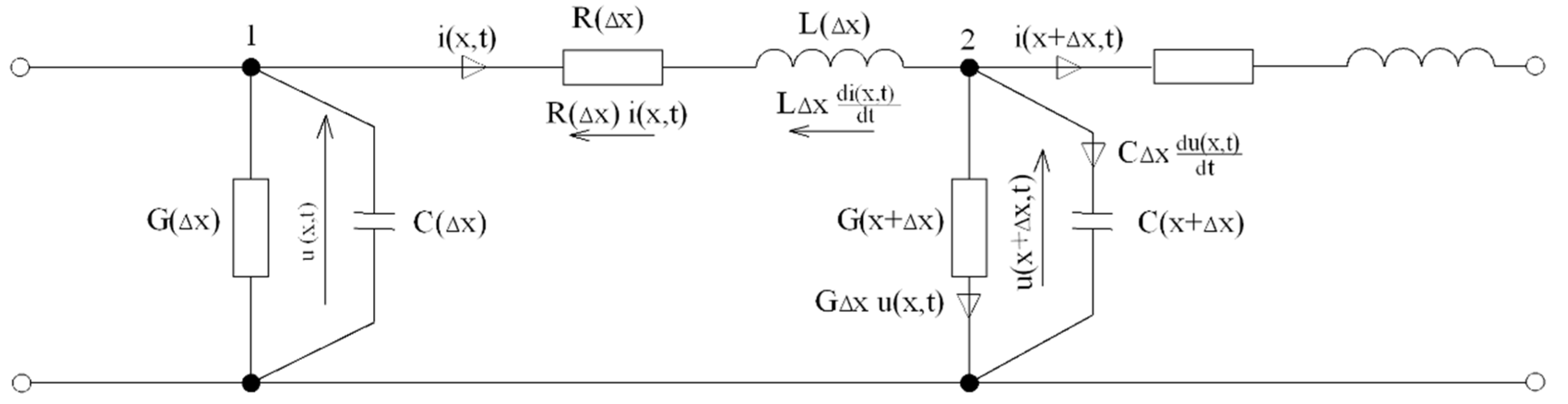
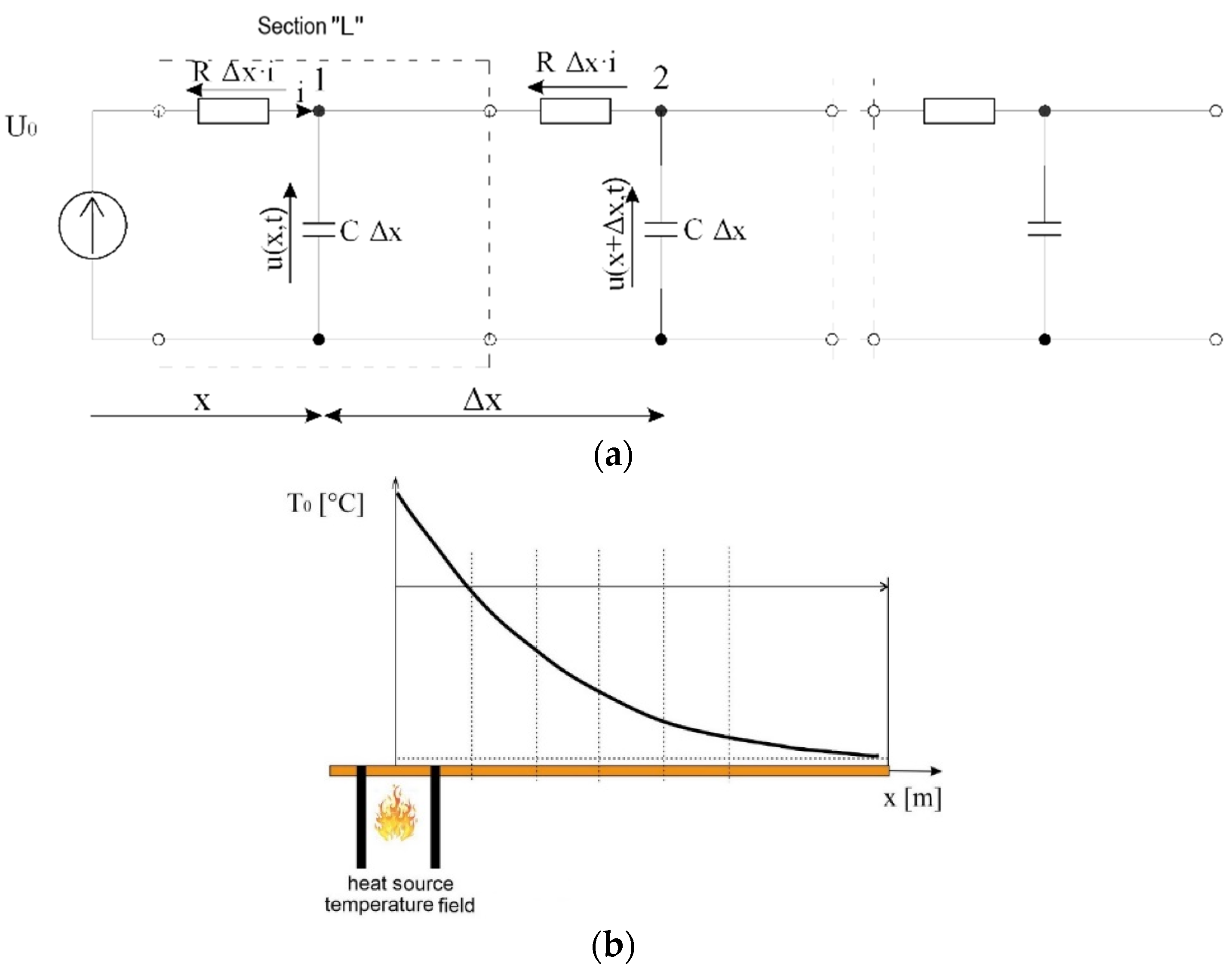
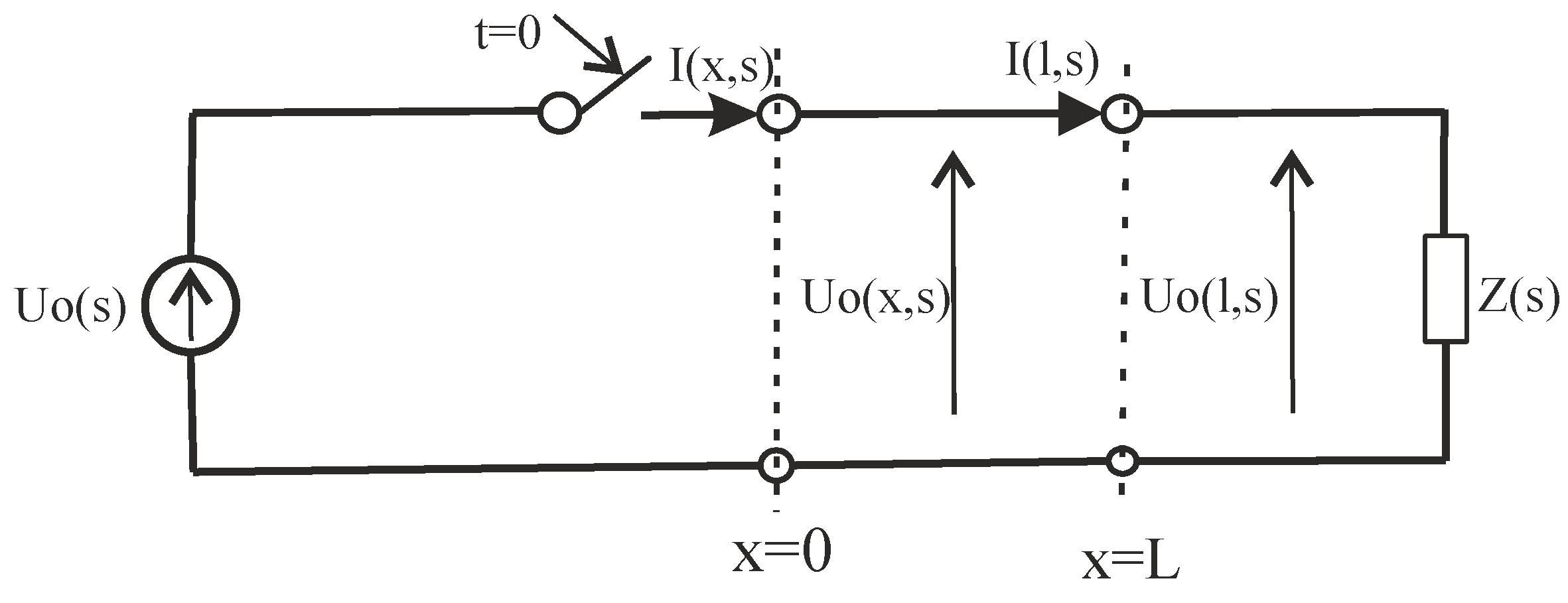
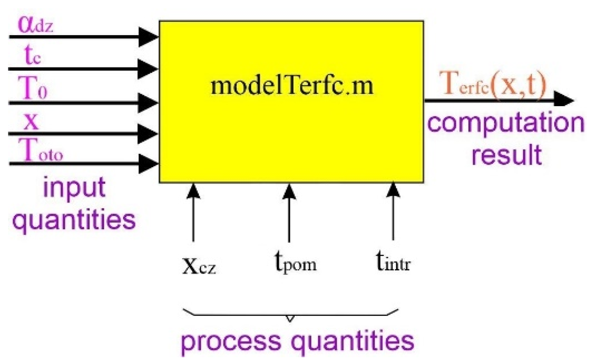
3. Modelling the Heating Up of Electrical Cables

An equation describing a transmission line shown in Figure 1 was used for the mathematical description. The solution to this equation, which assumes a lack of inductance and transverse conductivity of the line, is a model equation called the Thomson cable equation. It is a 2D model, and the parameters depend on time t and position x, and an external heat source is the forced input. A graphic solution to the model equation is a family of temperature curves with an exponential course that decreases with increasing distance from the heat source. Each curve presents a cable temperature profile for successive heating time values. Applying a thermo-electric analogy to electrical line equations allows us to model a cable heating process. This method enables the modelling of low-frequency thermal processes with lumped parameter elements [10,11]. Using the equation solution for a long electrical line and applying the analogy will enable us to obtain a temperature distribution for an electrical cable under the thermal conditions of a fire.

The Thomson transmission line variant assumes taking the longitudinal resistance and transverse capacitance of the line into account, while line transverse capacitance is omitted. A cable electrical system can then be shown as a quadripole composed of RC elements. Resistance R corresponds to the cable thermal resistance, and transverse heat losses refer to capacitance C (Figure 2a) [12,13,14,15].

Pursuant to Kirchhof’s 2nd law, the following can be written for the diagram shown in Figure 1:

$$i\left(x,t\right)-G \mathsf{\Delta }x·u\left(x,t\right)-C \mathsf{\Delta }x \frac{du\left(x,t\right)}{dt}-i\left(x+\mathsf{\Delta }x,t\right)=0,$$

(1)

According to Kirchhof’s 1st law, for node 2 we obtain:

$$u\left(x,t\right)-R \mathsf{\Delta }x·i\left(x,t\right)-L \mathsf{\Delta }x \frac{di\left(x,t\right)}{dt}-u\left(x+\mathsf{\Delta }x,t\right)=0,$$

(2)

where u(x, t) and i(x, t) are, respectively, the line voltage and current at a distance x from the source; R∆x and G∆x are the resistance and conductance of the elementary line segment; di(x, t)/dt and idu(x, t)/dt are, respectively, the change in the line voltage and current depending on the distance x from the source; u(x + ∆x, t) and i(x + ∆x, t) are the voltage and the current at any point in the line; C∆x du(x, t)/dt is the leakage current on the capacitance between the line cables; and L∆x di(x, t)/dt is the voltage loss due to the magnetic field of the long line. An electrical cable used for the experimental studies was divided into 15 equal elementary segments (Figure 2b). Each elementary segment is shown as a single “L”-type quadripole. For a line shown as a chain of the quadripole, the number increases indefinitely while the parameters of individual quadripoles simultaneously decrease, so it can be concluded that voltage and current at any point of the chain have a waveform similar to the source (forcing) signal.

For a line shown as a chain of a quadripole, the number of which increases indefinitely with the simultaneously decreasing parameters of individual quadripoles, it can be concluded that voltage and current have a waveform similar to the source (forcing) signal at any point of the chain.

For a line shown as a chain of a quadripole, the number of which increases indefinitely with simultaneously decreasing parameters of individual quadripoles, it can be concluded that voltage and current have a waveform similar to the source (forcing) signal at any point of the chain [16].

Based on the adopted assumptions, a cable’s thermal system can be presented as an electric quadripole consisting of RC elements [17,18]. Thermal resistance is modelled by resistance R, and transverse heat losses are represented by capacitance C [19]. The presented model uses a transmission line variant called the Thomson–Kelvin transmission line, which has the parameters L = G = 0 [20,21,22].

In order to determine a u(x, t) voltage equation, it is possible to apply the T(x, t) temperature waveform equation by analogy and use the Laplace transform of Equations (1) and (2) and present them in operator form

$$u-ℒ\left\{\frac{du}{dx}\right\}=R·I\left(x, s\right)+Lℒ\left\{\frac{di}{dt}\right\},$$

(3)

$$-ℒ\left\{\frac{di}{dx}\right\}=G·U\left(x, s\right)+Cℒ\left\{\frac{du}{dt}\right\},$$

(4)

where L{du/dx} and L{di/dx} are the Laplace transforms of the partial derivative over time for voltage and current, respectively; I(x, s) and U(x, s) are the Laplace transforms on the long line of current and voltage, respectively; and s is the Laplace transform operator. The voltage and current equation transforms take the form [23,24,25]

$$U\left(x, s\right)=ℒ\left\{u\left(x, t\right)\right\},$$

(5)

$$I\left(x, s\right)=ℒ\left\{i\left(x, t\right)\right\},$$

(6)

By applying the derivative transformation theorem to the Laplace transform, it can be started that [26,27]:

If function f(t) and its derivative F’(t) satisfy the conditions for Laplace transform and F(s) = $ℒ$ {f(t)}, then

$$ℒ\left\{f^{\prime }\left(t\right)\right\}=m\left[F\left(s\right)-\frac{f\left(0^{+}\right)}{s}\right]=sF\left(s\right)-f\left(0^{+}\right),$$

(7)

where m is the coefficient resulting from the Laplace transformation of the function u(t), and n stands for the number of the sequential derivative. While f(0)⁺ is the right-hand limit of the f(t) function at point t = 0. If function f(t) and its derivatives up to the n_th inclusive satisfy the conditions for the existence of the Laplace transform, then

$$ℒ\left\{f^{\left(n\right)}\left(t\right)\right\}=m^n\left[F\left(s\right)-\frac{f\left(0^{+}\right)}{s}-\frac{f^{\prime }\left(0^{+}\right)}{s^2}-\dots -\frac{f^{n-1}\left(0^{+}\right)}{s^n}\right],$$

(8)

By differentiating Equations (3) and (4) relative to x, we obtain

$$-\frac{dU}{dx}-{\gamma }^{2}U\left(x, s\right)=0,$$

(9)

where:

$$u\gamma =\gamma \left(s\right)=\sqrt{\left(R+sL\right)\left(G+sC\right)},$$

(10)

is the transmission line wave transfer constant, and γ is the wave transfer constant of the long line. Because s is a complex number, in order to obtain uniqueness, we assume that Re(γ) > 0.

The solution to the differential Equation (9) takes the form

$$U\left(x, s\right)=A_1{e}^{-\gamma x}+A_2{e}^{\gamma x},$$

(11)

where A₁ and A₂ are integration constants, which are determined based on boundary conditions.

Equation (11) is satisfied by the functions $\underset{\_}{U}=\underset{\_}{A_1}{e}^{-\gamma x}$ and $\underset{\_}{U}=\underset{\_}{A_2}{e}^{\gamma x}$, where constants A₁ and A₂ are integration constants. Due to the analogy between the temperature and electric voltage, the further course of reasoning will be limited to the voltage equation.

A temperature excitation within the experiment was of a stepwise nature, which, in the case of an electrical system, corresponds to supplying direct voltage to a line with infinite length (Figure 3). Given the assumption that Re[γ(s)] > 0, the Equation (11) reduces to the term $\underset{\_}{A_1}{e}^{-\gamma x}$.

We assumed that component A₂ = 0, otherwise the U(x, s) value would increase to infinity, which is physically impossible.

We introduced voltage U₀(s) at the beginning of the line, at moment t = 0, and hence, the U(0, s) = U₀(s) equation is the boundary condition. Based on the equation (11), we can determine A₁ = U₀(s), then the voltage transform within the line in question is expressed by the equation [28,29]

$$U\left(x, s\right)=U_0\left(s\right)e^{-\gamma x},$$

(12)

By substituting L = 0 and G = 0 to the relationship (10) we obtain a Kelvin line wave transfer constant relationship, which takes the form [30]

$$\gamma =\sqrt{sCR},$$

(13)

in that case, Equation (12) takes the form

$$U\left(x, s\right)=\frac{U_0}{s}{e}^{-x\sqrt{sCR}},$$

(14)

Under the assumption that U₀(s) = U₀/s, we achieve

$$u\left(x, s\right)=U_0{ℒ}^{-1}\left\{\frac{1}{s}{e}^{-x\sqrt{sCR}}\right\},$$

(15)

where ${ℒ}^{-1}$ is an inverse Laplace transform operation. By using tabular Laplace transforms, we obtain

$${ℒ}^{-1}\left\{\frac{1}{s}{e}^{-\alpha \sqrt{s}}\right\}=erfc\frac{\alpha }{2\sqrt{t}},$$

(16)

where the erfc(x) function is determined by the equation

$$u erfc\left(x\right)=\frac{2}{\sqrt{\pi }}{\int }_x^{\infty }{e}^{-u^2}du,$$

(17)

A solution to the voltage Equation (15) is a Thomson–Kelvin transmission line equation, which shows the voltage waveform in a transmission line that is one-sidedly limited and at a stepwise U₀ DC voltage activation, which has the form

$$\left(x,t\right)=U_0·erfc\left(\frac{x}{2}\sqrt{\frac{RC}{t}}\right),$$

(18)

where U₀ (V) is the excitation voltage, x (m) is the distance from the excitation source, R (Ω) is the electric resistance of the line, C (F) is the electric capacitance of the line, and t (s) is the excitation input time U₀.

In the case of Equation (18), after replacing the voltage value with the temperature value by analogy, we obtain model Equation (19) to calculate the heating temperature of the cable impacted by ambient temperature.

$$T\left(x,t\right)=T_0·erfc\left(\frac{x}{2}\sqrt{\frac{RC}{t}}\right),$$

(19)

The value of the erfc(x, t) function argument determines the value of the temperature signal damping element.

There ae various model input values, such as the:

(a)

Equivalent cable heat diffusion coefficient α_dz;

(b)

Impact time of an external temperature source t_c;

(c)

Distance x from the heat source, calculated along the cable longitudinal axis;

(d)

Cable ambient temperature T_oto;

(e)

Impact temperature of an external temperature field T₀.

The values introduced the developed experimental data model to enable the determination of the substitute R and C values, which measure the losses within a cable-environment thermal system.

A value that is significant from the model computation result accuracy perspective is the introduction of ambient temperature value T_oto. Ambient temperature is introduced as a mean value for the entire cable length. Assuming that a mean temperature along the cable length is not a breach since the process of calculating temperature inside buildings usually involves adopting a certain set of temperature values, most are usually in the range of 20–25 °C [31].

The computation algorithm converts a set of input quantities, namely experimental data originating from the heating process that characterized by a set of process quantities that do not directly participate in the computation algorithm but that determine the input values (Figure 4), such as:

(a)

Distance between measuring sensors x_cz;

(b)

Total experiment time t_pom;

(c)

Time step interval value t_intr.

Introducing measurement data into a computation script is preceded by the point estimation of the recorded wire temperature waveforms over successive time steps. The fit (fitted curve) computation model is responsible for that matter in Matlab software. The accuracy of the experimental data point estimation further influences data approximation for the T_erfc(x, t) model.

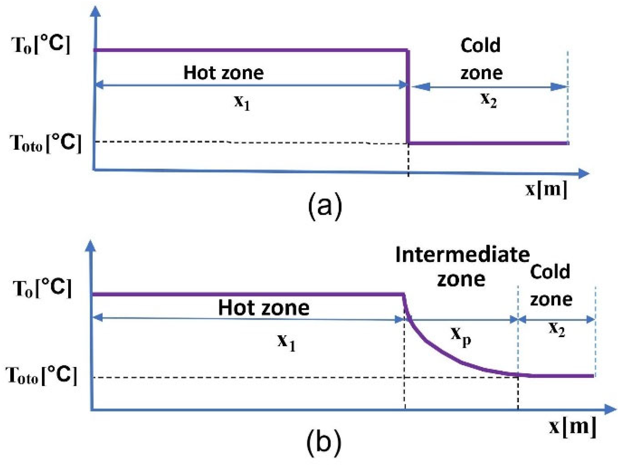
4. Determining Heating Temperature Curves

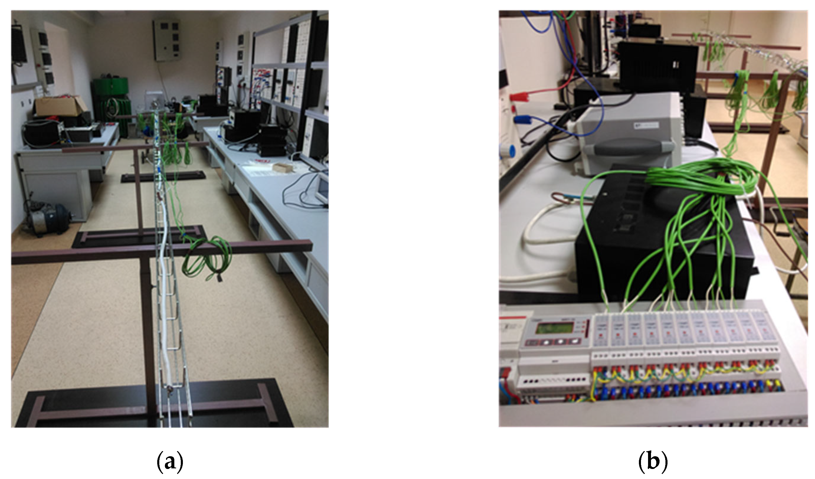
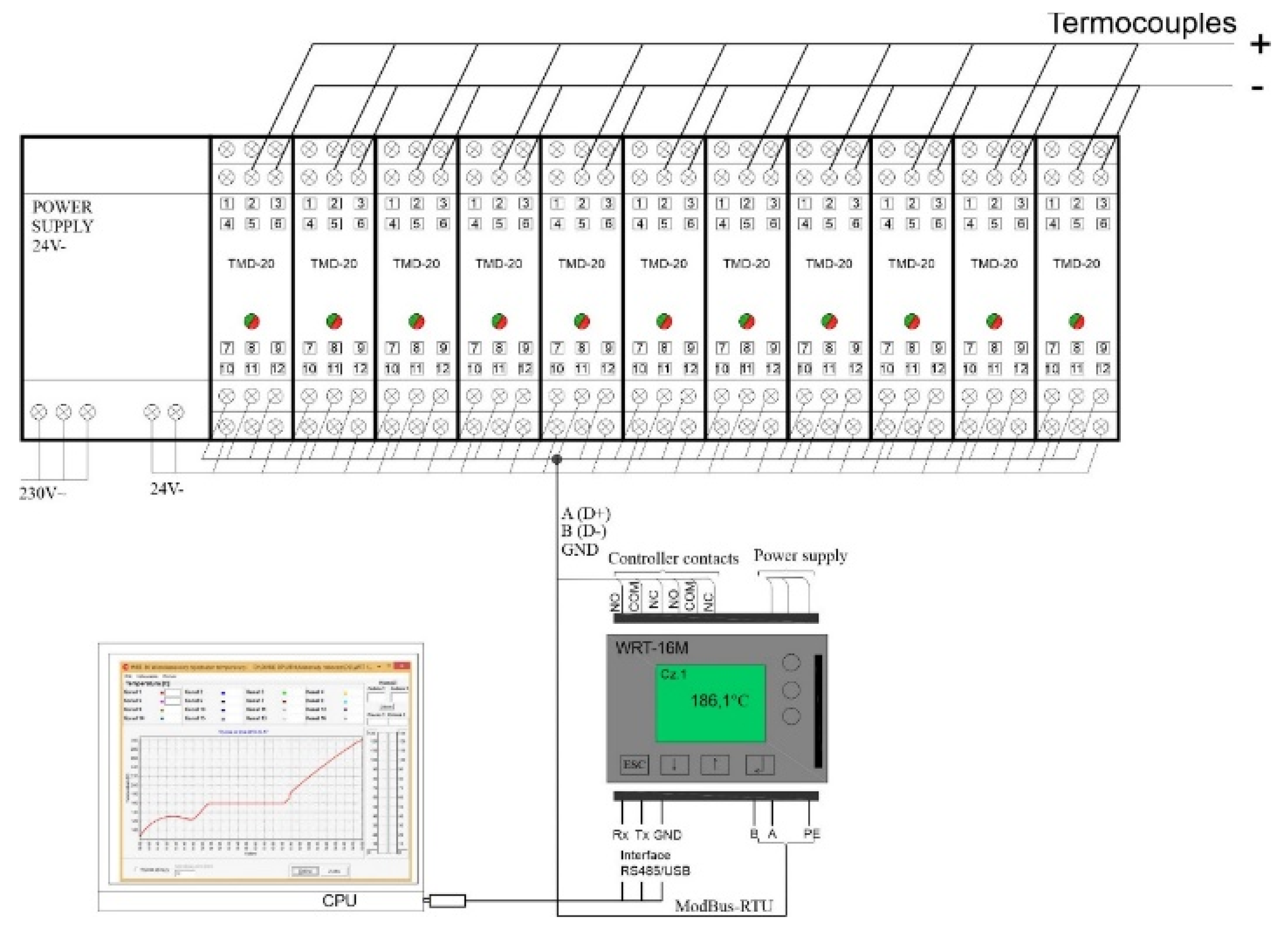
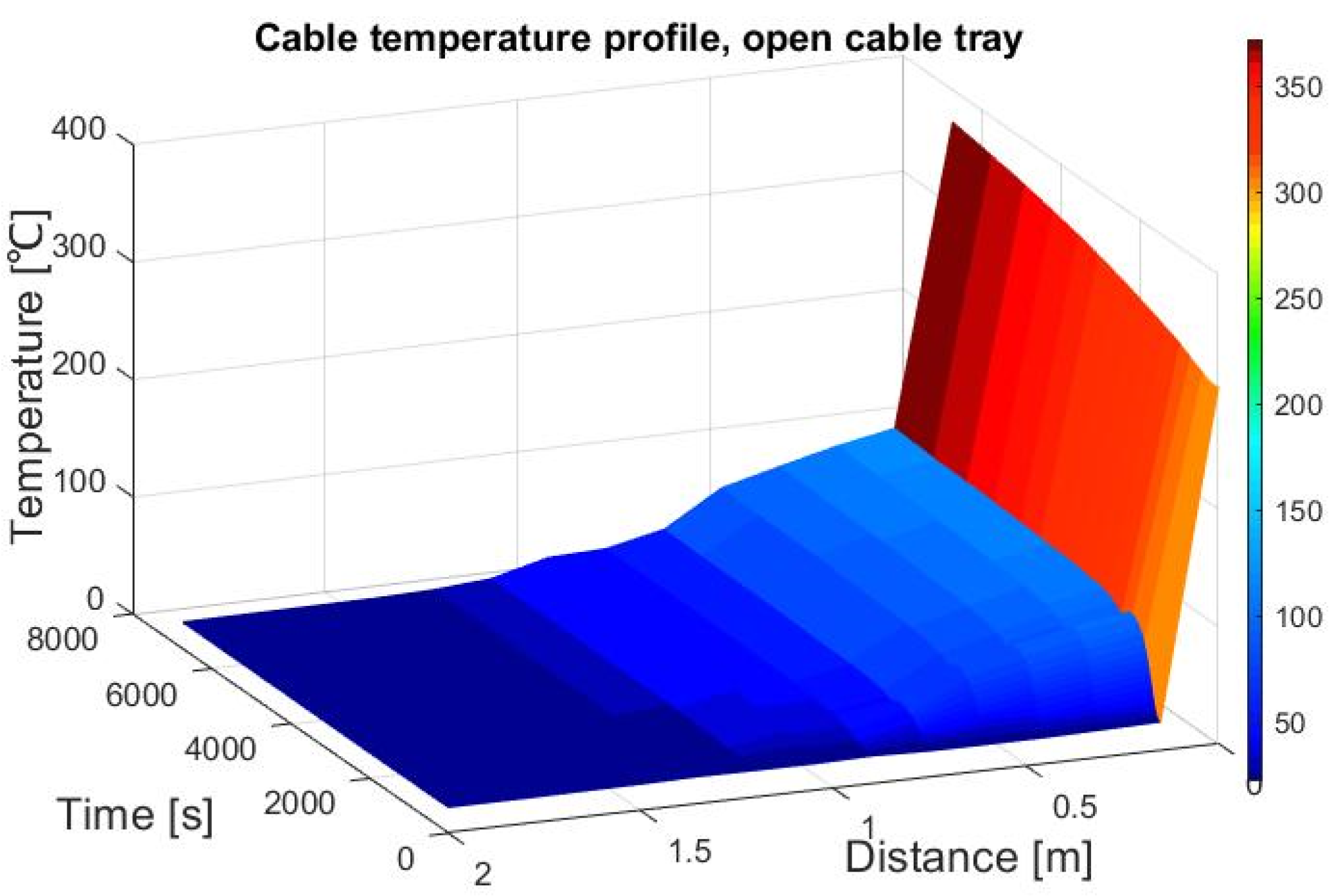
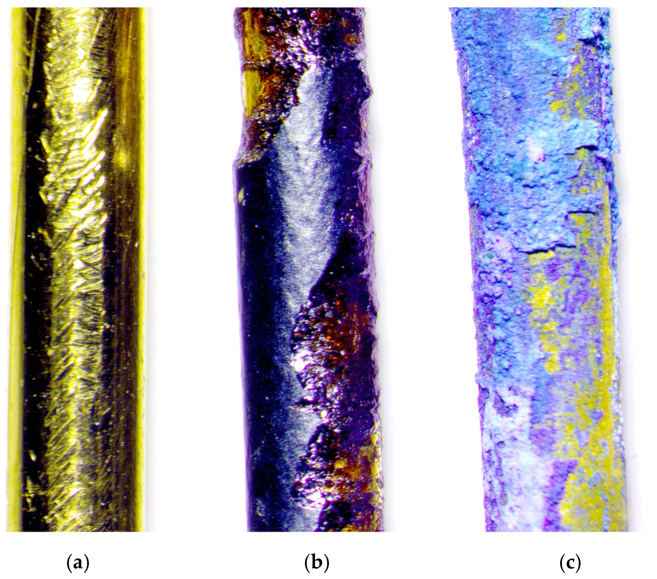
Due to the adopted preliminary assumptions as well as the model classification and structure, it is important to determine the parameters influencing the cable heating and cooling process. These parameters include the thermal resistance of the conductor R, insulation thermal capacity C, and the thermal diffusion coefficient α_dz.

The cable ambient temperature in the course of the conducted tests amounted to 22 °C (±2 °C). A temperature of 22 °C was adopted for the calculations. The time step values can have any t_intr interval. The experiment was executed over 7200 s, and the temperature was recorded every 2 s. Implementing the aforementioned data into the modelTerfc.m computation mode enabled us to obtain a family of curves showing the temperature distribution along the longitudinal axis of a non-flammable cable (Figure 5).

Determining the equivalent heat losses R and C from the cable to the environment is a very important stage for calculating the T_erfc(x, t) model determined by Equation (14). They impact the shape of the model temperature curves and the process accuracy of the temperature modelling as a function of time and distance from the heat source [6,32].

Each curve is a longitudinal temperature distribution for a conductive wire of an electrical cable at a given time from 100 s to 3000 s from the time of excitation.

The simulation time fell in the range of 0–120 min, which is in line with the standard fire duration. The thermal coefficients of halide-free cable material components are shown in

Table 1. Thermal coefficients of the components of studied cable.

Material	Thermal Conductivity Coefficient	Specific Heat Capacity
Copper	399	380
Mica	0.523	1800
Polyethylene	0.25	1000
XLPE	0.25	1000
HFFR insulation	0.25	1000

.

5. Test Bench

K-type thermocouples were used to measure the temperature of the conductors. The method utilizing thermo-elements is beneficial because of the structural possibilities of thermocouple sensors, measurement accuracy, and the option to utilize the obtained measurement results in further calculations.

The test bench consists of a laboratory tube furnace with a 100 cm-long heating zone that is made entirely of a heat-resistant quartz glass tube. The hot zone is heated via a 3.2 kW induction heater. The furnace is heated and controlled through a micro-processor temperature controller. Temperature settings are programmed in a control block.

Another part of the test bench, which requires designing, is the system that measures and records the obtained results. The experimental tests utilized a measuring system consisting of 14 K-type thermocouples (TP-203-K-300-10), 14 programmable TMD-20 measurement transducers, and a 16-channel WRT-16M temperature recorder. A diagram of the system is shown in Figure 6.

The system required the transducers to be programmed in terms of the type of used thermocouples and the length of the measurement connection cables (10 m long cables were used). Measurement signals from measurement transducers are sent to the recorder via a ModBus-RTU serial bus. The data from the transducers were read in the WRT-16M temperature recorder. An RS485/USB interface ensured communication with the recorder.

The measurement transducers are coupled in a single line with taps (Figure 7). The sensor-connecting cable has shielded signal conductors (LiYCY 2 × 0.34 mm²), which makes it resistant to the action of electromagnetic fields. Prior to connection, a transducer must be configured and assigned a unique address in the form of a number from 1 to 70.

Air humidity and ambient temperature were measured using a PWT-401 hytherograph. The measurement data were recorded as a text file. The ambient temperature did not change in the course of the test, with an average of 22.2 °C, while the mean humidity was 38.9%.

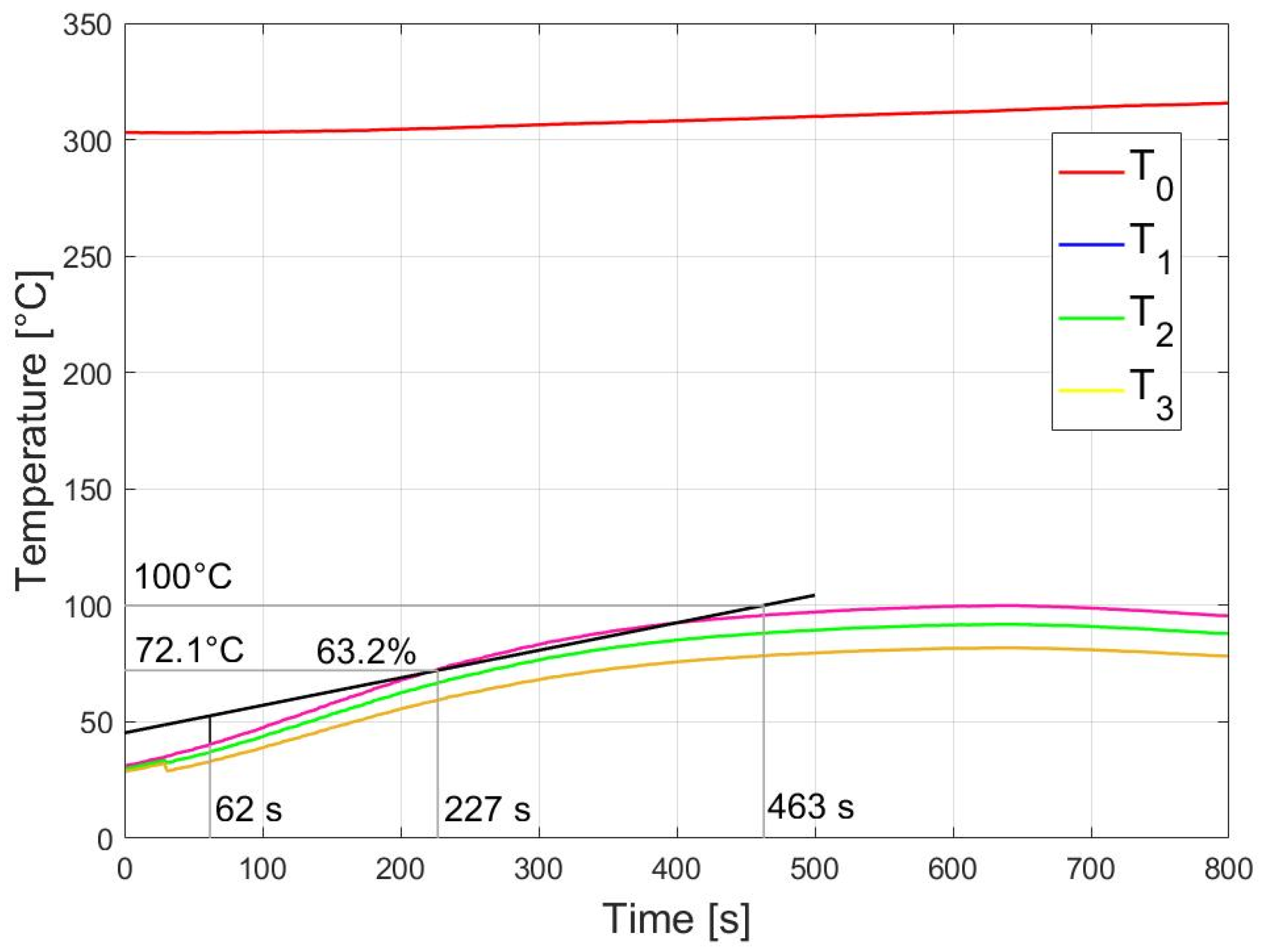
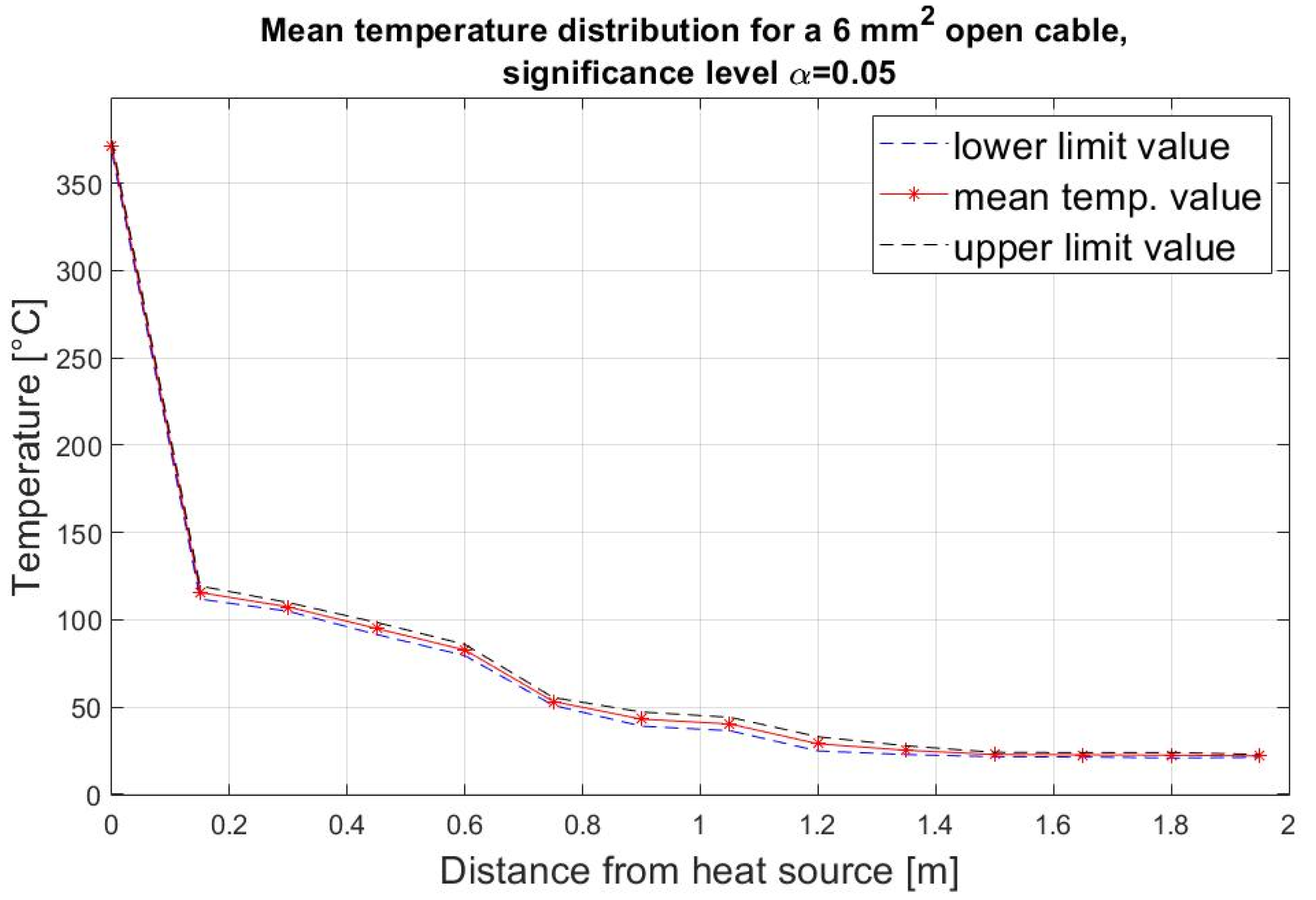
6. Research Experiment Result Analysis

The analysis of the experimentally obtained temperature curves describing the studied cable enabled an observation that a cable subjected to the action of a temperature field (e.g., a fire) exhibits a transition zone, where the temperature changes from the temperature forcing heating to a temperature not affected by such a field. A cable in a fire-free zone is exposed to ambient temperature or, in an extreme case, a continuous permissible temperature that is caused by a flowing current with a continuously permissible value. A method utilizing the conductor resistance increase coefficient k_R is used commonly for engineering purposes, depending on the adopted approximate length of the hot zone relative to the total cable length. This method does not assume the existence of an intermediate zone (Figure 8), where the cable temperature significantly exceeds the permissible values at a certain section.

It should be noted that the intermediate zone occurs in both directions from the heat source along the cable’s longitudinal axis. The experiments conducted within this study assumed and involved executing temperature measurements in one direction along the cable.

The temperature was measured every 2 s, which provided 3600 measurement samples for a 120 min test duration. The ambient temperature and humidity as well as the dew point were measured simultaneously to measure the core temperature of the cable. A set of results for each time instant with recorded temperature enabled the development of a cable temperature profile after 120 min of heating, which is shown in Figure 9.

The result for the core temperature measurements along the cable length reflect the electrical cable heating process, e.g., during fires, not only in the zone directly exposed to the temperature but also as a result of the heat being conducted by the electrical cables. The obtained test results enabled the verification of the R and C parameter values in the heat conductivity model.

This does not provide a full picture of the cable temperature profile; thus, this assumption is insufficient for modelling the heating of halogen-free flame-retardant cables.

An analysis of the surface graph shown in Figure 9, which is a cable temperature profile, enabling the observation of two stages in the heating process involving the copper conductors in a cable. At the first stage, the wire temperature increases due to it being exposed to temperatures in the furnace heating chamber. This increase is a response to the step excitation, which can be described by time and amplitude parameters. The time parameters describe response dynamics, while the amplitude parameters describe the post-excitation response value. The nature of the response time is determined by response time latency (so-called dead top time) and the response signal time constant (τc).

The top delay time determines an object’s response to a change induced by an excitation signal. The time constant τc determines the time after which an object, with a change induced by the excitation signal, reaches a new steady state.

Further computations adopted a time constant τ = 463 s. The time constant value was determined by the tangent method and is represented in Figure 10. It was also assumed that the steady state would appear after approximately four time constants (1600 s) from the start of the heating process [33].

Measurement series results were subjected to Student’s t-distribution in order to calculate the measurement error. The determined measurement error, at a significance level of α = 0.05, was adopted in the simulation and is marked in Figure 11.

The estimated mean cable temperature value and measurement error for a set level of significance in the intermediate zone were calculated based on a fourfold temperature measurement during heating [34].

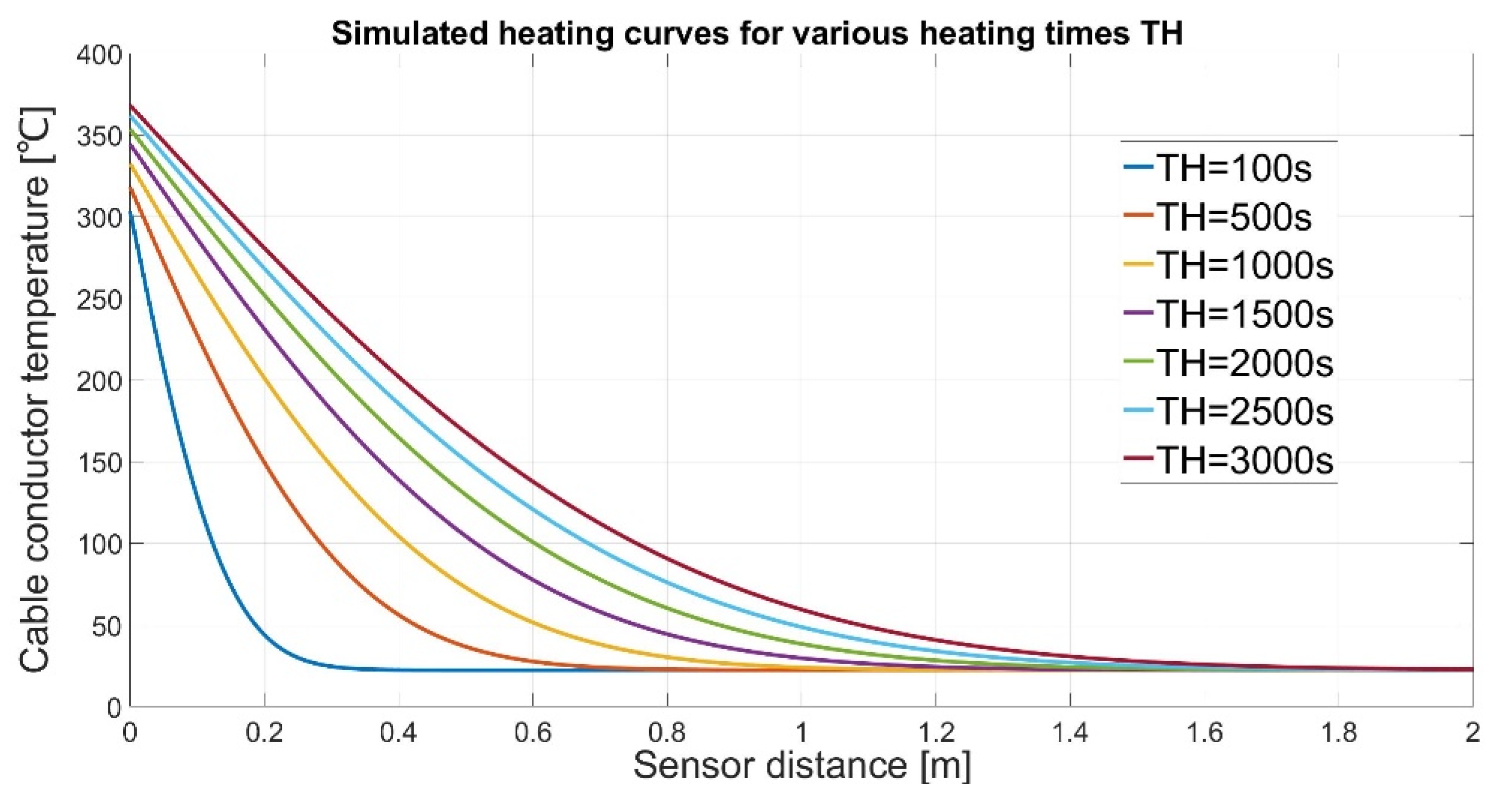
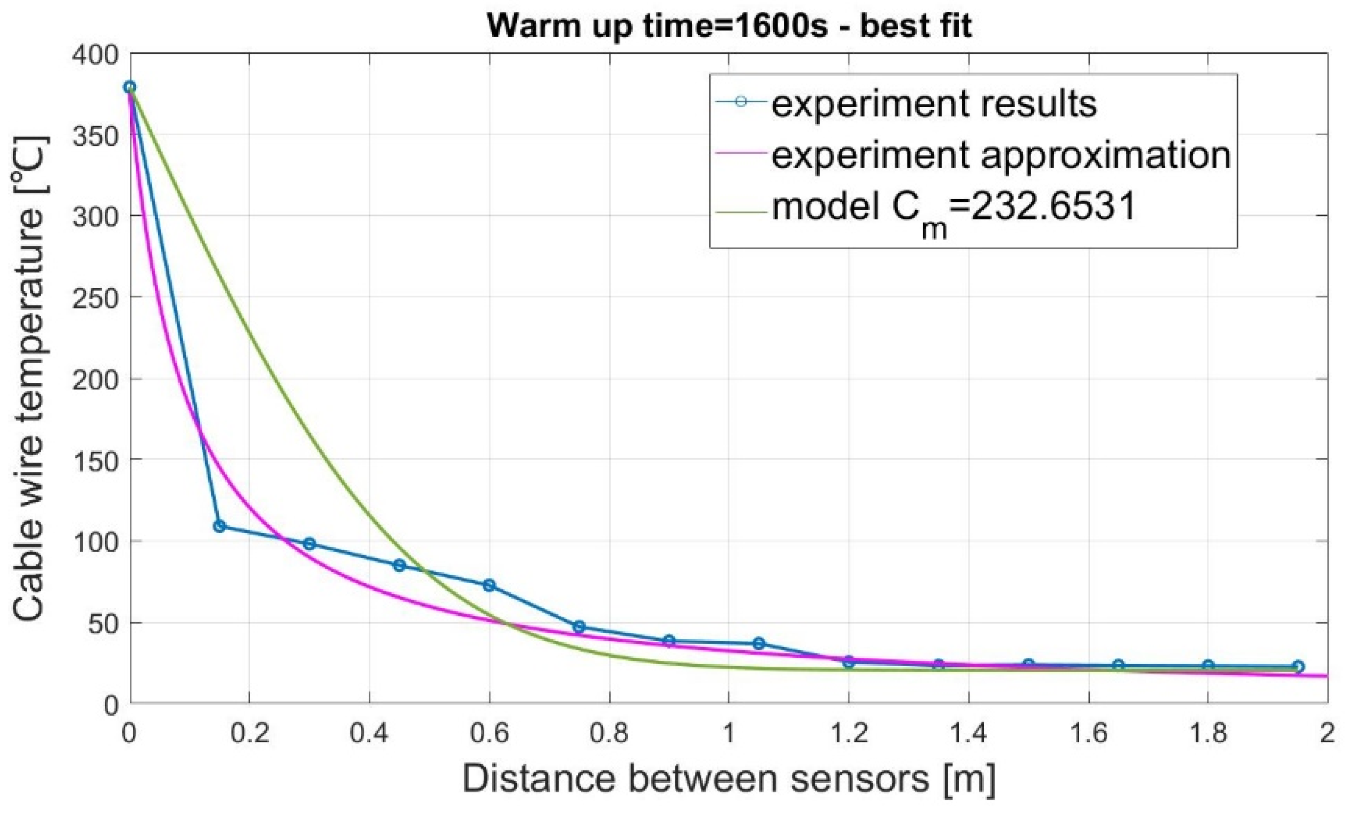
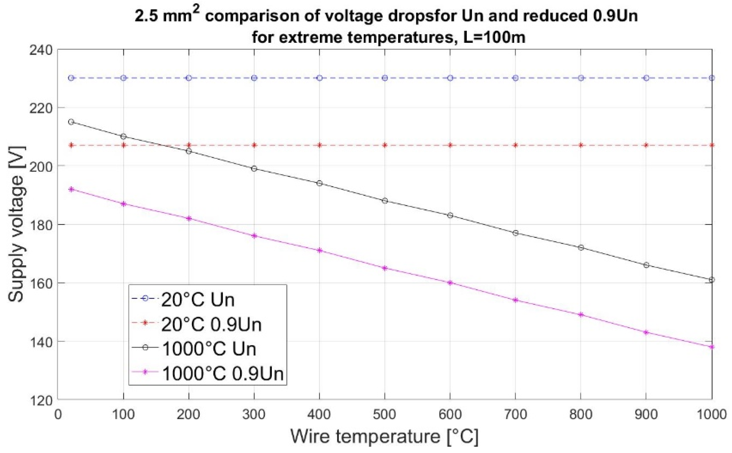
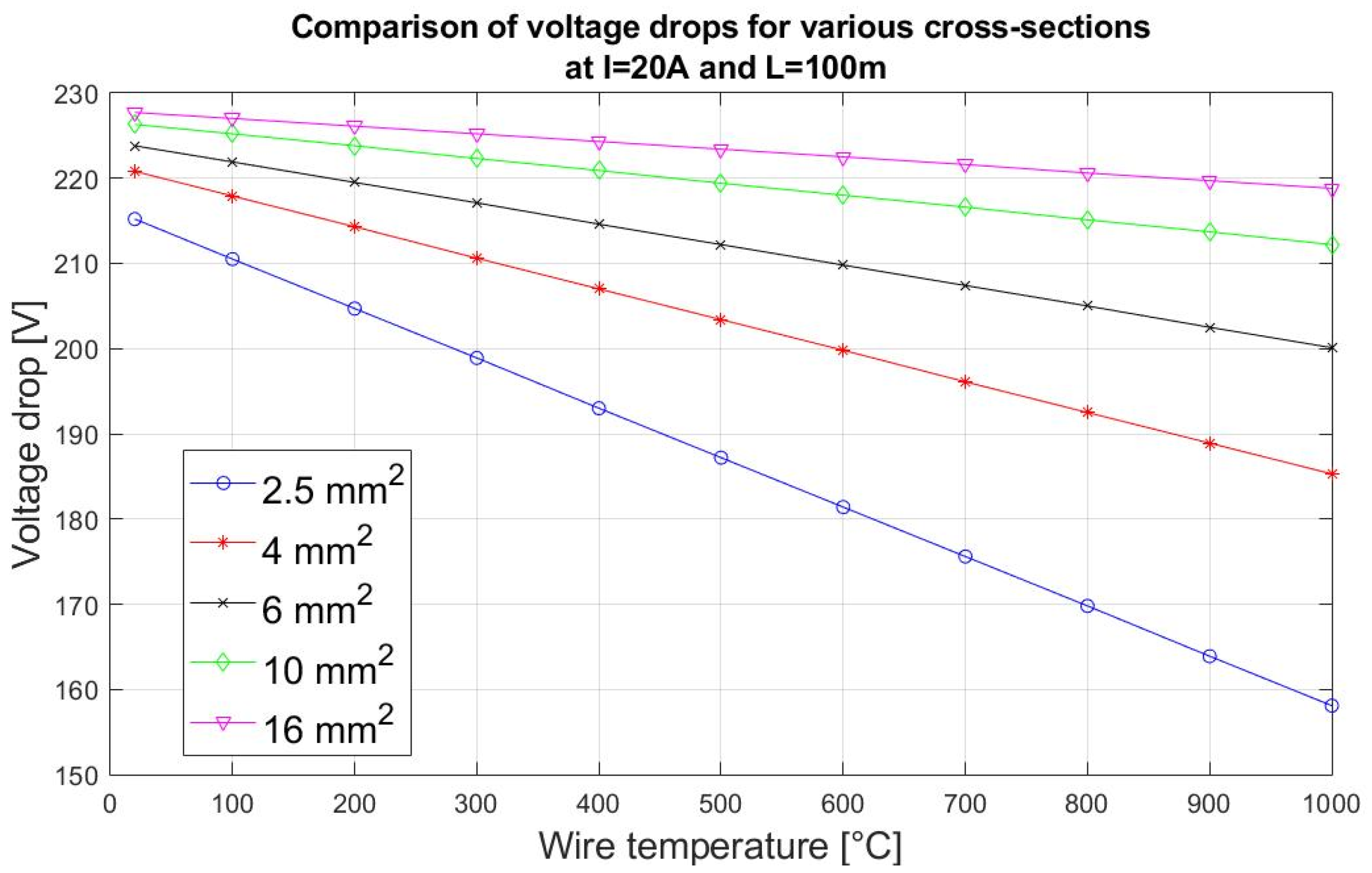
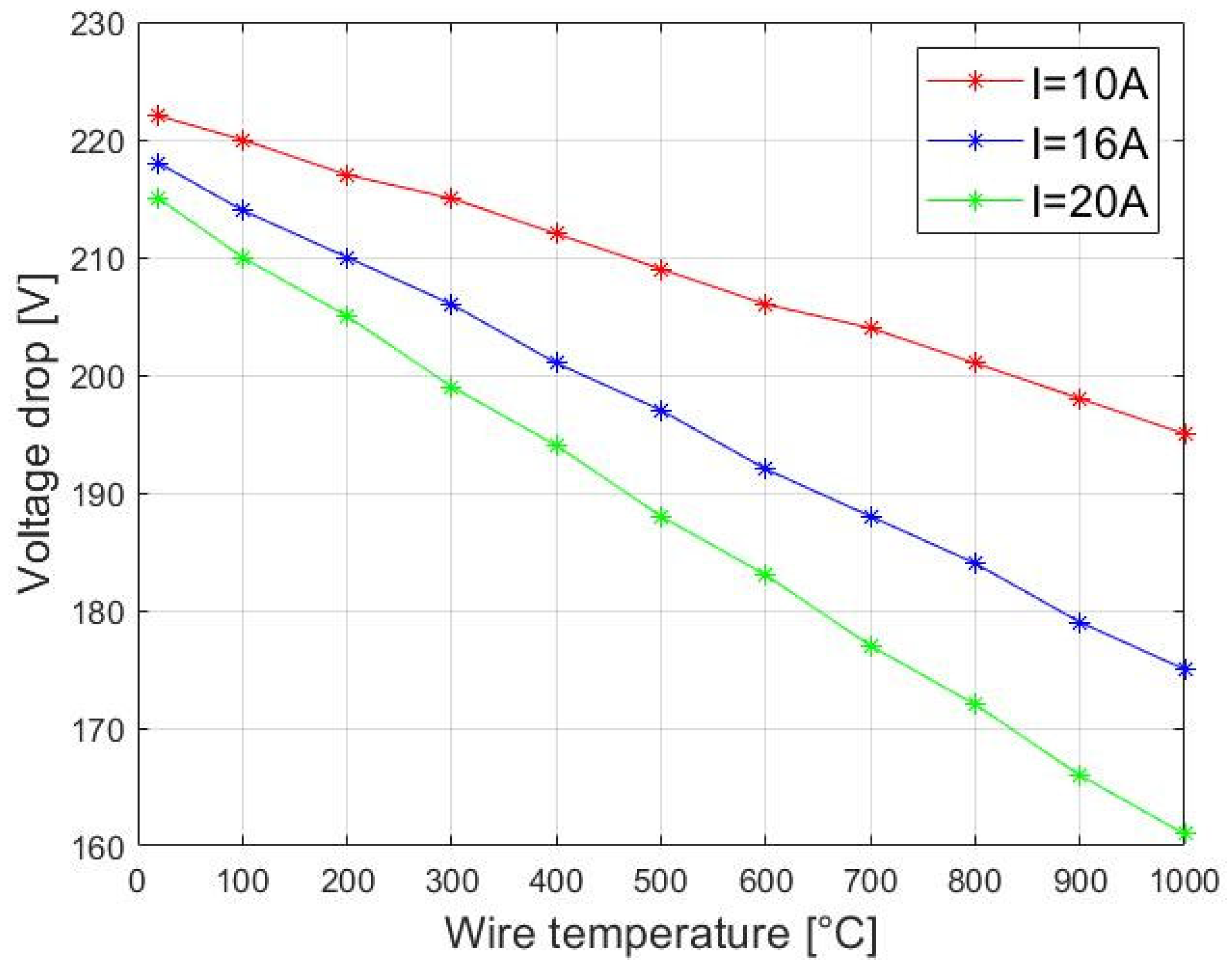
7. Simulation Model Result Analysis

Measurement results for the steady state time instant indicate that the change of the temperature along the cable is similar to the exponential signal damping. The damping intensity depends on the thermal resistance of the conductor and the thermal capacity of the electrical insulation. It was assumed that the thermal resistance of the conductor was fixed and independent of temperature. Figure 12 shows an experimental temperature curve for a time of 1600 s and a curve plotted by the model.

The authors approximated the model curve for the experiment using an exponential function via the Levenberg–Marquadt algorithm and obtained the heat capacity value of C_m = 232 (J/kg·K), for which the model curve best matched the experimental curve (Figure 12).

The conducted computation simulations enabled the determination of the multiplicity of the cable resistance increase depending on their temperature and voltage drops within the tested cable. The simulation computations presented in Figure 13 show that the resistance of copper installation cables R_T in a temperature range of 20 °C-1000 °C increases fivefold, regardless of the cable cross-section. Increasing resistance entails a supply voltage drop within the cable.

The conducted simulation showed that the supply voltage drop within the cable, at a temperature of 1000 °C, and a current load equal to 20 A amounted to 30% relative to the rated value U_n. A similar drop also occurred in the case of the rated reduced permissible voltage U_nd, which is shown in Figure 13.

Electrical cables exposed to the temperature field of a fire experience temperature degradation resulting from the insulation and conductor material.

Figure 14 shows a comparison of the surfaces of the conductors made of copper prior to and after heating (a), and (b) shows that the conductor cross-section changes after heating. The conductor cross-section changes due to wire surface oxidation, resulting in a part of the wire materials changing into copper oxide CuO(II), which is a much worse electricity conductor than the conductor copper CU ETP.

The measured cross-section reduction after 120 min of cable heating was approximately 20% relative to the conductor cross-section prior to heating.

It is a significant reduction of the cable’s transmission capacity that results in a reduced permissible current-carrying capacity and an additional voltage drop in the cable.

The simulation computations (Figure 15) enable an assessment of the ability of a cable to satisfy the requirement regarding the power supply of fire-fighting equipment during a fire, which is assumed in the standard (e.g., electric motor of a fire-water pump). The voltage simulation drops for various cable cross-sections and assumes a supply line with a length of L = 100 m. In the cases of the 2.5 mm² and 4 mm² cables, the temperature boundary at which the permissible voltage drop is exceeded, and the power supply isolated by the protections is 400 °C and 700 °C, respectively.

The appearance of additional cable resistance impairs the reliability of conditions and the power supply. The supply voltage drop on fire pump terminals leads to an adequate drop of the current transmission capacity of the cables. Figure 16 shows a voltage drop simulation that depends on the current load of the line supplying fire-fighting equipment.

A start-up of an unloaded motor results in the decrease of its power factor and a significant increase in the starting current, which, in turn, further deepens the voltage drop in the motor’s supply circuit during start-up. The higher the power of the supplied motor, the greater the drop. Therefore, exceeding the permissible voltage drop value on the terminals of a motor can lead to stalling.

8. Conclusions

The article discusses issues associated with studying the physical and chemical properties in electrical cables as systems supplying fire-fighting equipment. The authors describe a mathematical model for cable heating along with a simulated cable temperature distribution and an evaluation of the impact of temperature on conductor resistance and the cable’s current-carrying capacity.

The work presents a heat flow phenomenon in electrical cables. Electrical systems were compared to thermal systems through analogy, and a method for solving a partial differential voltage equation based on distributed parameters was used.

The following conclusions can be drawn from the conducted experimental and simulation tests:

(a)

The method based on applying the theory distributed parameters to solve a partial differential voltage equation of a transmission line resulted in a solution that can be used as a theoretical model of temperature distribution in electrical cables;

(b)

The knowledge of temperature values and distribution within the hot and intermediate zones of the cable enabled the calculation of the increase in the resistance of the cables exposed to a temperature field;

(c)

Failure to take the intermediate zone into account leads to an incorrect determination of the actual voltage drop in an electrical cable;

(d)

Determining the thermal parameters of a cable and the time parameters of the heating process enabled the determination of the increase in the resistance of the cable caused by an external temperature excitation;

(e)

The value of the excitation temperature and heating time is decisive in terms of determining the impact of temperature on the resistance of evaluated cables.

In the presented model, some simplifications were adopted, such as: material homogeneity, no material defects, and the same cross-section along the entire length of the cable. These simplifications cause minor errors by idealizing the research object, but with the current technological level and the continuous development of engineering and material technology, these errors are negligible. The model is designed for the slow heating of cables to the order of tens of minutes, with the assumption of a stable and continuous process of the uniform heating of the area covered by the heat source. In the future, it will be necessary to develop another model and to build a stand that takes into account the process of more rapid and uneven heating. Despite these limitations, the developed model, as a results of conducted study, can support a risk analysis covering the fire hazard to people and buildings both at the design and operation stage of already existing facilities. Current methods of designing a fire protection system often oversize the cross-section of the cables, which increases the cost and size of the installation. As devices and structures are designed with appropriate safety features, including the fire protection system, from the beginning, the use of the proposed model f to determine the temperature of cables may allow the transfer of funds to other elements of the project. This can result, for example, in increasing the efficiency of the system and reducing its complexity as well as optimizing its entire structure, with the original amount of financial resources and maintaining the same safety standards. The conclusions and guidelines contained herein can be benefited from by both construction designers and researchers dealing with studies in the field of electrical system fire safety.

References

1. Enescu, D.; Colella, P.; Russo, A. Thermal Assessment of Power Cables and Impacts on Cable Current Rating: An Overview. Energies 2020, 13, 5319. [Google Scholar] [CrossRef]
2. Novak, B.; Tamus, Z.Á.; Koller, L. Heating of Cables Due to Fault Currents. In Proceedings of the 2010 IEEE International Symposium on Electrical Insulation, San Diego, CA, USA, 6–9 June 2010. [Google Scholar] [CrossRef]
3. Ocłoń, P.; Pobędza, J.; Walczak, P.; Cisek, P.; Vallati, A. Experimental Validation of a Heat Transfer Model in Underground Power Cable Systems. Energies 2020, 13, 1747. [Google Scholar] [CrossRef] [Green Version]
4. Perka, B.; Suproniuk, M.; Piwowarski, K. Application of acoustic surface wave to measure bus bar temperature. Prz. Elektrotechniczny 2019, 95, 120–123. [Google Scholar] [CrossRef]
5. Szczegielniak, T.; Kusiak, D.; Jabłoński, P. Thermal Analysis of the Medium Voltage Cable. Energies 2021, 14, 4164. [Google Scholar] [CrossRef]
6. Ghoneim, S.S.M.; Mahrouse, A.; Nehmdoh, A.S. Transient Thermal Performance of Power Cable Ascertained Using Finite Element Analysis. Processes 2021, 9, 438. [Google Scholar] [CrossRef]
7. Jörgens, C.; Clemens, M. Electric Field and Temperature Simulations of High-Voltage Direct Current Cables Considering the Soil Environment. Energies 2021, 14, 4910. [Google Scholar] [CrossRef]
8. Plesca, A. Temperature Distribution of HBC Fuses with Asymmetric Electric Current Ratios Through Fuselinks. Energies 2018, 11, 1990. [Google Scholar] [CrossRef] [Green Version]
9. DIN. DIN 4102-12. In Behavior of Building Materials and Elements under the Influence of Fire. Maintaining the Functions of Devices during a Fire. Requirements and Tests; DIN: Berlin, Germany, 1998. [Google Scholar]
10. Al–Saud, M.S. Assessment of thermal performance of underground current carrying conductors. IET Gener. Transm. Distrib. 2011, 5, 630–639. [Google Scholar] [CrossRef]
11. Granieri, P.P. Heat transfer through cable insulation of Nb-Ti superconducting magnets operating in He II. Cryog. J. 2012, 53, 61–71. [Google Scholar] [CrossRef] [Green Version]
12. Anders, G.J.; Napieralski, A.; Kulesza, Z. Calculation of the internal thermal resistance and ampacity of 3-core screened cables with fillers. IEEE Trans. Power Deliv. 1999, 14, 729–734. [Google Scholar] [CrossRef]
13. Bejan, A.; Kraus, A.D. Heat Transfer Handbook; Wiley: New York, NY, USA, 2003. [Google Scholar]
14. Hanna, M.A.; Baxter, C.; Baxter, M.; Salama, M.M.A. Thermal modelling of cables in conduits: (Air gap consideration). In Proceedings of the 1995 Canadian Conference on Electrical and Computer Engineering (CCECEYCCGEI ’95), Montreal, QC, Canada, 5–8 September 1995; pp. 578–581. [Google Scholar] [CrossRef]
15. Hiraiwa, Y.; Kasubuchi, T. Temperature dependence of thermal conductivity of soil over a wide range of temperature (5–75 °C). Eur. J. Soil Sci. 2000, 51, 211–218. [Google Scholar] [CrossRef]
16. Brakelmann, H.; Anders, G.J.; Cherukupalli, S. Mitigation of a Hot Spot Along a Cable Circuit Using a Novel Cooling Solution. IEEE Trans. Power Deliv. 2020, 35, 592–599. [Google Scholar] [CrossRef]
17. Chenzao, F.; Wenrong, S.; Lingyu, Z.; Hongle, L.; Zhoufeil, Y.; Yilin, W. Research on the fast calculation model for transient temperature rise of direct buried cable groups. In Proceedings of the 2018 12th International Conference on the Properties and Applications of Dielectric Materials (ICPADM), Xi’an, China, 20–24 May 2018; pp. 646–652. [Google Scholar] [CrossRef]
18. Hui, Z.; Quing, C.; Haofei, S. Study on Temperature Field of Cable Tunnel Fire. In Proceedings of the 2019 9th International Conference on Fire Science and Fire Protection Engineering (ICFSFPE), Chengdu, China, 18–20 October 2019. [Google Scholar] [CrossRef]
19. Packa, J.; Durman, V.; Sulova, J. Behaviour of Fire Resistant Cable Insulation with Different Flame Barriers During Water Immersion. In Proceedings of the 2019 20th International Scientific Conference on Electric Power Engineering (EPE), Kouty nad Desnou, Czech Republic, 29 July 2019. [Google Scholar] [CrossRef]
20. Ren, Y.; Wu, K.; Coker, D.F.; Quirke, N. Thermal transport in model copper-polyethylene interfaces. J. Chem. Phys. 2019, 151, 174708. [Google Scholar] [CrossRef] [PubMed]
21. Robertson, A.F.; Gross, D. An Electrical—Analog method for Transient Heat-Flow Analisis. J. Res. Natl. Stand. 1958, 61, 2892. [Google Scholar]
22. Sarajcev, I.; Majstrovic, M.; Medic, I. Calculation of losses in electric power cables as the base for cable temperaturę analysis. WIT Trans. Eng. Sci. 2000, 29, 9. [Google Scholar] [CrossRef]
23. Olsen, R.; Anders, G.J.; Holboell, J.; Gudmundsdottir, U.S. Modelling of Dynamic Transmission Cable Temperature Considering Soil-Specific Heat, Thermal Resistivity, and Precipitation. IEEE Trans. Power Deliv. 2013, 28, 1909–1917. [Google Scholar] [CrossRef] [Green Version]
24. Suproniuk, M.; Pawlowski, M.; Wierzbowski, M.; Majda-Zdancewicz, E.; Pawlowski, M. Comparison of methods applied in photoinduced transient spectroscopy to determining the defect center parameters: The correlation procedure and the signal analysis based on inverse Laplace transformation. Rev. Sci. Instrum. 2018, 89, 044702. [Google Scholar] [CrossRef] [PubMed]
25. Goga, V.; Paulech, J.; Wary, M. Cooling of electrical Cu conductor with PVC insulation-analytical, numerical and fluid flow solution. J. Electr. Eng. 2013, 64, 92–99. [Google Scholar] [CrossRef] [Green Version]
26. Nakayama, W. Heat-transfer engineering in systems integration: Outlook for closer coupling of thermal and electrical designs of computers. IEEE Trans. Compon. Packag. Manuf. Technol. Part A 1995, 18, 818–826. [Google Scholar] [CrossRef]
27. Purushothaman, S.; de León, F.; Terracciano, M. Calculation of cable thermal rating considering non-isothermal earth surface. IET Gener. Transmiss. Distrib. 2014, 8, 1354–1361. [Google Scholar] [CrossRef] [Green Version]
28. Wang, Z.; Karniadakis, G.E.; Chalafant, J.; Chryssostomidis, C.; Babaee, H. High-fidelity modeling and optimization of conjugate heat transfer in arrays of heated cables. In Proceedings of the 2017 IEEE Electric Ship Technologies Symposium (ESTS), Arlington, VA, USA, 14–17 August 2017; pp. 557–563. [Google Scholar] [CrossRef]
29. Garrido, C.; Antonio, F.O.; Cidras, J. Theoretical model to calculate steady-state and transient ampacity and temperature in buried cables. IEEE Trans. Power Deliv. 2003, 18, 667–678. [Google Scholar] [CrossRef]
30. Gang, L.; LEI Ming, R.; Banyi, Z.; Fan, L.; Yinghong, L.Y. Model Research of Real-time Calculation for Single-core Cable. Temperature Considering Axial Heat Transfer. Gaodianya Jishu/High Volt. Eng. 2012, 38, 1877–1883. [Google Scholar] [CrossRef]
31. Suproniuk, M.; Pas, J. Analysis of electrical energy consumption in a public utility buildings. Prz. Elektrotechniczny 2019, 95, 97–100. [Google Scholar] [CrossRef]
32. Desmet, J.; Putman, D.; Vanalme, G.; Belmans, R.; Vandommelent, D. Thermal analysis of parallel underground energy cables. In Proceedings of the CIRED 2005—18th International Conference and Exhibition on Electricity, Distribution, Turin, Italy, 6–9 June 2005; pp. 1–4. [Google Scholar] [CrossRef]
33. Ariyanayagam, A.D.; Mahen Mahendran, M. Energy Based Time Equivalent Approach to Determine the Fire Resistance Ratings of Light Gauge Steel Frame Walls Exposed to Realistic Design Fire Curves. J. Struct. Fire Eng. 2017, 8, 46–72. [Google Scholar]
34. Zhao, H.C.; Lyall, J.S.; Nourbakhsh, G. Probabilistic cable rating based on cable thermal environment studying. In Proceedings of the PowerCon International Conference on Power System Technology (Cat. No.00EX409), Perth, Australia, 4–7 December 2000; Volume 2, pp. 1071–1076. [Google Scholar] [CrossRef] [Green Version]
Figure 1. Application of Kirchhof’s law to a transmission line fragment.
Energies 14 07260 g001
Figure 2. Sketch showing an electrical cable division (a) into L-type quadripole sections; (b) into measuring sections for time t1.
Energies 14 07260 g002
Figure 3. Supplying DC voltage to a line of infinite length.
Energies 14 07260 g003
Figure 4. Identification of Terfc(x, t) model signals.
Energies 14 07260 g004
Figure 5. Temperature curve model simulation.
Energies 14 07260 g005
Figure 6. View of the test bench for heating electrical cables: (a) cable in a cable tray; (b) temperature transducers and recorder.
Energies 14 07260 g006
Figure 7. Measuring and recording block diagram.
Energies 14 07260 g007
Figure 8. Cable division into thermal zones: (a) commonly used for the computations, (b) actual. Toto is a cable ambient temperature, T0 is an impact temperature of an external temperature field, x1 is the length of the hot zone, x2 is the length of the cold zone, and xp is the length of the intermediate zone.
Energies 14 07260 g008
Figure 9. Temperature profile in an open cable tray after 120 min of heating. Temperatures recorded at measuring points placed along the cable enabled the determination of cable heating time constants.
Energies 14 07260 g009
Figure 10. Time constant determined using the “tangent” method. T0 is an impact temperature of an external temperature field, T1 is the temperature measured at a place 0.2 m away from the heat source, T2 is the temperature measured at a place 0.4 m away from the heat source, and T3 is the temperature measured at a place 0.6 m away from the heat source. The black line is the mark’s tangent, and the gray lines are the guidelines.
Energies 14 07260 g010
Figure 11. Cable temperature curve obtained through a measurement experiment depending on the distance from the heat source.
Energies 14 07260 g011
Figure 12. Plotted temperature curve best matching the experiment.
Energies 14 07260 g012
Figure 13. Simulated voltage drop depending on the cable temperature.
Energies 14 07260 g013
Figure 14. View of conductor surface (a) prior to heating, (b) after 120 min of heating, and (c) after cooling down to 25 °C.
Energies 14 07260 g014
Figure 15. Simulated voltage drops depending on the cable temperature and cross-section.
Energies 14 07260 g015
Figure 16. Simulated voltage drop for various current loads of cables.
Energies 14 07260 g016