
Identification of BDS Satellite Clock Periodic Signals Based on Lomb-Scargle Power Spectrum and Continuous Wavelet Transform

 , ,
, ,  and
and
Abstract
1. Introduction
2. Materials and Methods
2.1. Data Source
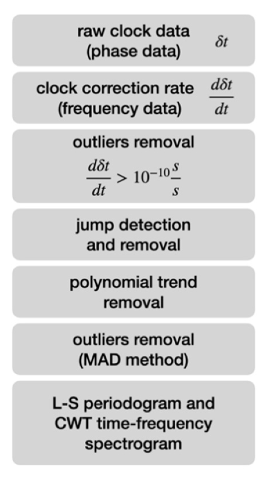
2.2. Methods
- represents the scale
- denotes the translation
- represents the mother wavelet, and * denotes the complex conjugate
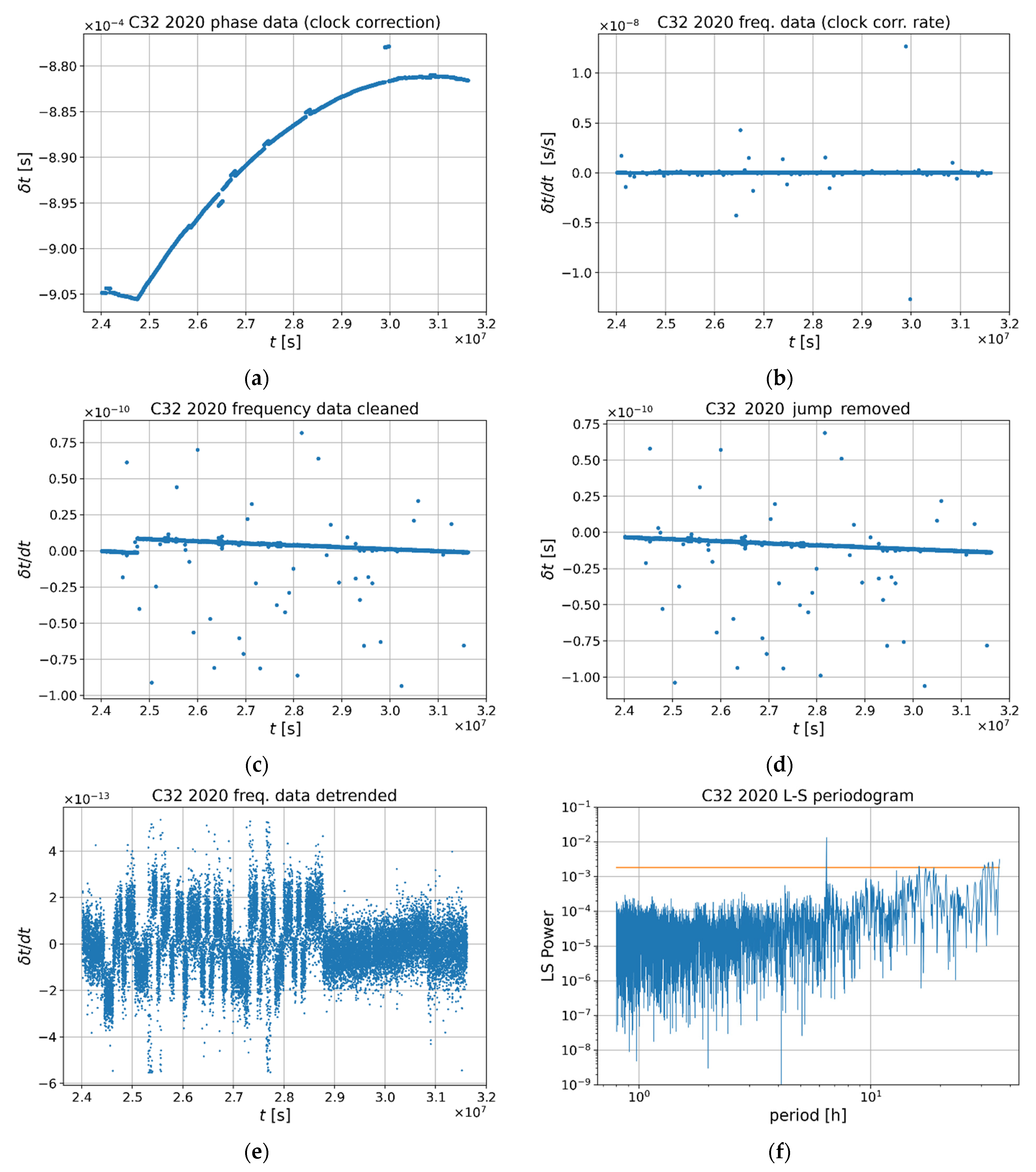
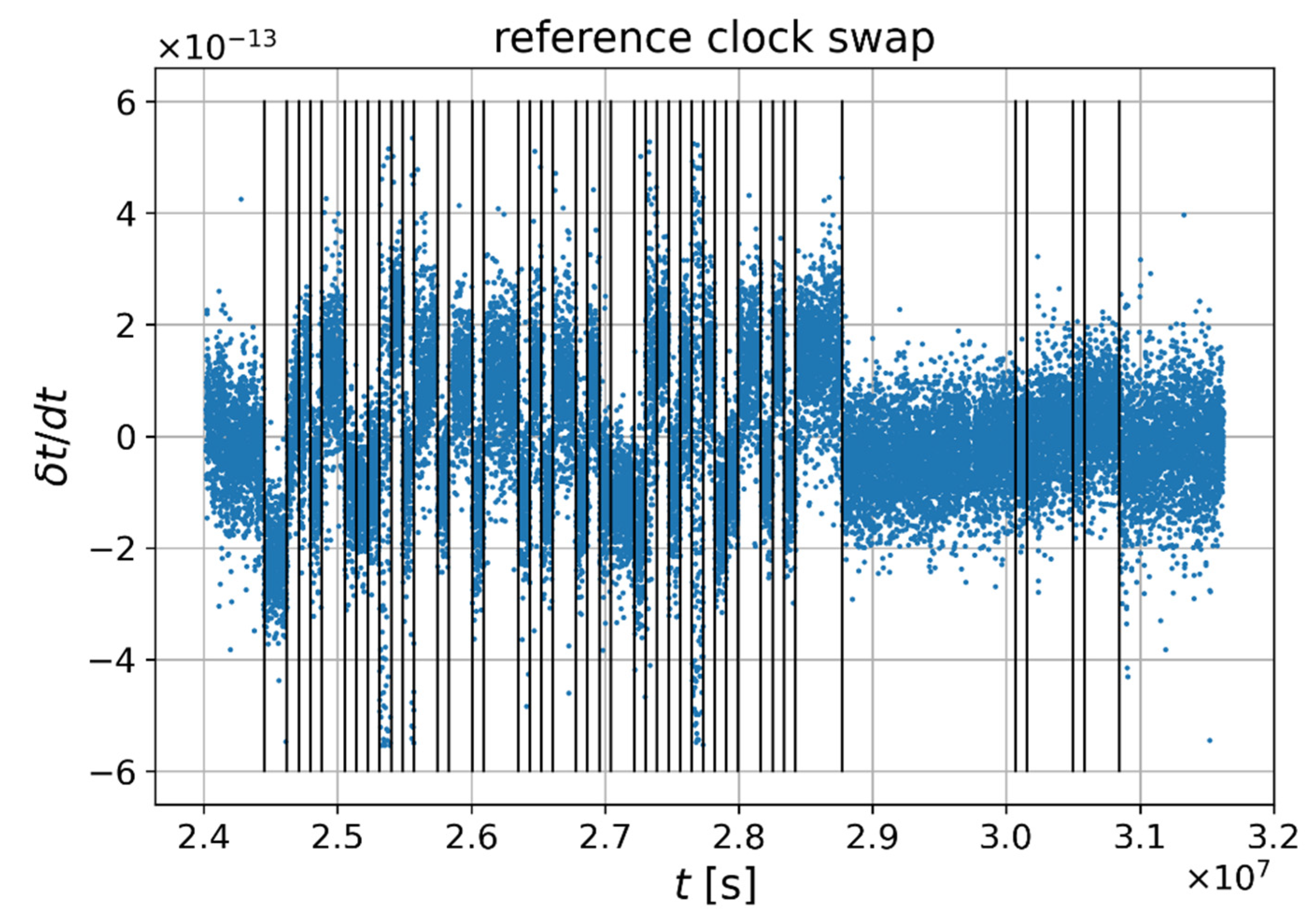
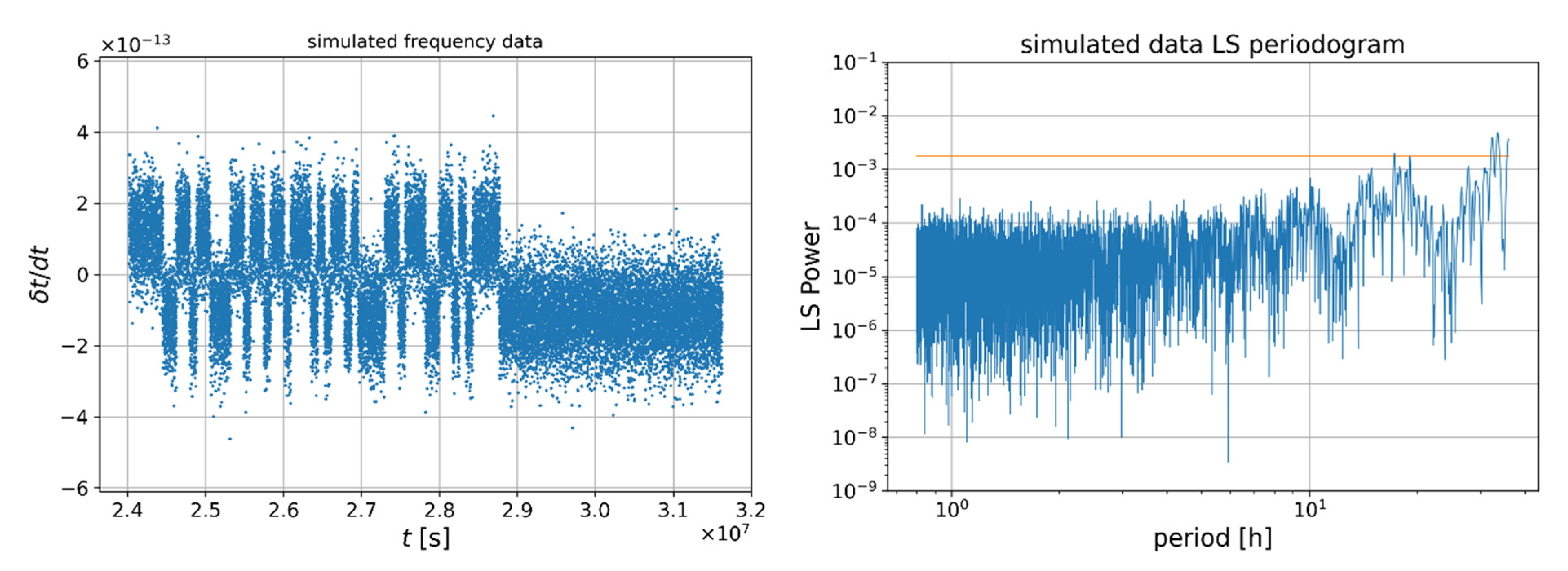
3. Results and Discussion
4. Conclusions
Author Contributions
Funding
Institutional Review Board Statement
Informed Consent Statement
Data Availability Statement
Conflicts of Interest
Appendix A

| PRN | IGS-SVN | NORADID | SVN | Satellite Type | Clock Type | Manuf | Launch Date | SatStatus | Healthy | Service Signal |
|---|---|---|---|---|---|---|---|---|---|---|
| 1 | C020 | 44231 | GEO-8 | BDS-2 | Rubidium | CASC | 17 May 2019 | Operational | Healthy | B1I/B2I/B3I |
| 2 | C016 | 38953 | GEO-6 | BDS-2 | Rubidium | CASC | 25 October 2012 | Operational | Healthy | B1I/B2I/B3I |
| 3 | C018 | 41586 | GEO-7 | BDS-2 | Rubidium | CASC | 12 June 2016 | Operational | Healthy | B1I/B2I/B3I |
| 4 | C006 | 37210 | GEO-4 | BDS-2 | Rubidium | CASC | 1 November 2010 | Operational | Healthy | B1I/B2I/B3I |
| 5 | C011 | 38091 | GEO-5 | BDS-2 | Rubidium | CASC | 25 February 2012 | Operational | Healthy | B1I/B2I/B3I |
| 6 | C005 | 36828 | IGSO-1 | BDS-2 | Rubidium | CASC | 1 August 2010 | Operational | Healthy | B1I/B2I/B3I |
| 7 | C007 | 37256 | IGSO-2 | BDS-2 | Rubidium | CASC | 18 December 2010 | Operational | Healthy | B1I/B2I/B3I |
| 8 | C008 | 37384 | IGSO-3 | BDS-2 | Rubidium | CASC | 10 April 2011 | Operational | Healthy | B1I/B2I/B3I |
| 9 | C009 | 37763 | IGSO-4 | BDS-2 | Rubidium | CASC | 27 July 2011 | Operational | Healthy | B1I/B2I/B3I |
| 10 | C010 | 37948 | IGSO-5 | BDS-2 | Rubidium | CASC | 2 December 2011 | Operational | Healthy | B1I/B2I/B3I |
| 11 | C012 | 38250 | MEO-3 | BDS-2 | Rubidium | CASC | 30 April 2012 | Operational | Healthy | B1I/B2I/B3I |
| 12 | C013 | 38251 | MEO-4 | BDS-2 | Rubidium | CASC | 30 April 2012 | Operational | Healthy | B1I/B2I/B3I |
| 13 | C017 | 41434 | IGSO-6 | BDS-2 | Rubidium | CASC | 30 March 2016 | Operational | Healthy | B1I/B2I/B3I |
| 14 | C015 | 38775 | MEO-6 | BDS-2 | Rubidium | CASC | 19 September 2012 | Operational | Healthy | B1I/B2I/B3I |
| 16 | C019 | 43539 | IGSO-7 | BDS-2 | Rubidium | CASC | 10 July 2018 | Operational | Healthy | B1I/B2I/B3I |
| 19 | C201 | 43001 | MEO-1 | BDS-3 | Rubidium | CASC | 5 November 2017 | Operational | Healthy | B1I/B3I/B1C/B2a/B2b |
| 20 | C202 | 43002 | MEO-2 | BDS-3 | Rubidium | CASC | 5 November 2017 | Operational | Healthy | B1I/B3I/B1C/B2a/B2b |
| 21 | C206 | 43208 | MEO-3 | BDS-3 | Rubidium | CASC | 12 February 2018 | Operational | Healthy | B1I/B3I/B1C/B2a/B2b |
| 22 | C205 | 43207 | MEO-4 | BDS-3 | Rubidium | CASC | 12 February 2018 | Operational | Healthy | B1I/B3I/B1C/B2a/B2b |
| 23 | C209 | 43581 | MEO-5 | BDS-3 | Rubidium | CASC | 29 July 2018 | Operational | Healthy | B1I/B3I/B1C/B2a/B2b |
| 24 | C210 | 43582 | MEO-6 | BDS-3 | Rubidium | CASC | 29 July 2018 | Operational | Healthy | B1I/B3I/B1C/B2a/B2b |
| 25 | C212 | 43603 | MEO-11 | BDS-3 | Hydrogen | SECM | 25 August 2018 | Operational | Healthy | B1I/B3I/B1C/B2a/B2b |
| 26 | C211 | 43602 | MEO-12 | BDS-3 | Hydrogen | SECM | 25 August 2018 | Operational | Healthy | B1I/B3I/B1C/B2a/B2b |
| 27 | C203 | 43107 | MEO-7 | BDS-3 | Hydrogen | SECM | 12 January 2018 | Operational | Healthy | B1I/B3I/B1C/B2a/B2b |
| 28 | C204 | 43108 | MEO-8 | BDS-3 | Hydrogen | SECM | 12 January 2018 | Operational | Healthy | B1I/B3I/B1C/B2a/B2b |
| 29 | C207 | 43245 | MEO-9 | BDS-3 | Hydrogen | SECM | 30 March 2018 | Operational | Healthy | B1I/B3I/B1C/B2a/B2b |
| 30 | C208 | 43246 | MEO-10 | BDS-3 | Hydrogen | SECM | 30 March 2018 | Operational | Healthy | B1I/B3I/B1C/B2a/B2b |
| 31 | C101 | 40549 | IGSO-1S | BDS-3S | Hydrogen | SECM | 30 March 2015 | Experiment | -- | -- |
| 32 | C213 | 43622 | MEO-13 | BDS-3 | Rubidium | CASC | 19 September 2018 | Operational | Healthy | B1I/B3I/B1C/B2a/B2b |
| 33 | C214 | 43623 | MEO-14 | BDS-3 | Rubidium | CASC | 19 September 2018 | Operational | Healthy | B1I/B3I/B1C/B2a/B2b |
| 34 | C216 | 43648 | MEO-15 | BDS-3 | Hydrogen | SECM | 15 October 2018 | Operational | Healthy | B1I/B3I/B1C/B2a/B2b |
| 35 | C215 | 43647 | MEO-16 | BDS-3 | Hydrogen | SECM | 15 October 2018 | Operational | Healthy | B1I/B3I/B1C/B2a/B2b |
| 36 | C218 | 43706 | MEO-17 | BDS-3 | Rubidium | CASC | 19 November 2018 | Operational | Healthy | B1I/B3I/B1C/B2a/B2b |
| 37 | C219 | 43707 | MEO-18 | BDS-3 | Rubidium | CASC | 19 November 2018 | Operational | Healthy | B1I/B3I/B1C/B2a/B2b |
| 38 | C220 | 44204 | IGSO-1 | BDS-3 | Hydrogen | CASC | 20 April 2019 | Operational | Healthy | B1I/B3I/B1C/B2a/B2b |
| 39 | C221 | 44337 | IGSO-2 | BDS-3 | Hydrogen | CASC | 25 June 2019 | Operational | Healthy | B1I/B3I/B1C/B2a/B2b |
| 40 | C224 | 44709 | IGSO-3 | BDS-3 | Hydrogen | CASC | 5 November 2019 | Operational | Healthy | B1I/B3I/B1C/B2a/B2b |
| 41 | C227 | 44864 | MEO-19 | BDS-3 | Hydrogen | CASC | 16 December 2019 | Operational | Healthy | B1I/B3I/B1C/B2a/B2b |
| 42 | C228 | 44865 | MEO-20 | BDS-3 | Hydrogen | CASC | 16 December 2019 | Operational | Healthy | B1I/B3I/B1C/B2a/B2b |
| 43 | C226 | 44794 | MEO-21 | BDS-3 | Hydrogen | SECM | 23 November 2019 | Operational | Healthy | B1I/B3I/B1C/B2a/B2b |
| 44 | C225 | 44793 | MEO-22 | BDS-3 | Hydrogen | SECM | 23 November 2019 | Operational | Healthy | B1I/B3I/B1C/B2a/B2b |
| 45 | C223 | 44543 | MEO-23 | BDS-3 | Rubidium | CASC | 23 September 2019 | Operational | Healthy | B1I/B3I/B1C/B2a/B2b |
| 46 | C222 | 44542 | MEO-24 | BDS-3 | Rubidium | CASC | 23 September 2019 | Operational | Healthy | B1I/B3I/B1C/B2a/B2b |
| 56 | C104 | 40938 | IGSO-2S | BDS-3S | Hydrogen | CASC | 30 September 2015 | Experiment | -- | -- |
| 57 | C102 | 40749 | MEO-1S | BDS-3S | Rubidium | CASC | 25 July 2015 | Experiment | -- | -- |
| 58 | C103 | 40748 | MEO-2S | BDS-3S | Rubidium | CASC | 25 July 2015 | Experiment | -- | -- |
| 59 | C217 | 43683 | GEO-1 | BDS-3 | Hydrogen | CASC | 1 November 2018 | Operational | Healthy | B1I/B3I |
| 60 | C229 | 45344 | GEO-2 | BDS-3 | Hydrogen | CASC | 9 March 2020 | Operational | Healthy | B1I/B3I |
| 61 | C230 | 45807 | GEO-3 | BDS-3 | Hydrogen | CASC | 23 June 2020 | Testing | -- | B1I/B3I |
Appendix B

Appendix C


Appendix D


References
- Su, K.; Jin, S.; Jiao, G. Assessment of multi-frequency GNSS PPP models using GPS, Beidou, GLONASS, Galileo and QZSS. Meas. Sci. Technol. 2020, in press. [Google Scholar] [CrossRef]
- Han, C.; Cai, Z. Relativistic effects to the onboard BeiDou satellite clocks. Navig. J. Inst. Navig. 2019, 66, 49–53. [Google Scholar] [CrossRef]
- Lewinska, P.; Dyczko, A.; Matula, R. Integration of Thermal Digital 3D Model and a MASW (Multichannel Analysis of Surface Wave) as a Means of Improving Monitoring of Spoil Tip Stability. In Proceedings of the 2017 Baltic Geodetic Congress (BGC Geomatics), Gdansk, Poland, 22–25 June 2017; pp. 232–236. [Google Scholar] [CrossRef]
- Lewińska, P.; Dyczko, A. Thermal digital terrain model of a coal spoil tip—A way of improving monitoring and early diagnostics of potential spontaneous combustion areas. J. Ecol. Eng. 2016, 17, 170–179. [Google Scholar] [CrossRef]
- Nistor, S. The influence of different types of noise on the velocity uncertainties in GPS time series analysis. Acta Geodyn. Geomater. 2016, 13, 387–394. [Google Scholar] [CrossRef][Green Version]
- Nistor, S.; Buda, A.S. Evaluation of the ambiguity resolution and data products from different analysis centers on zenith wet delay using PPP method. Acta Geodyn. Geomater. 2017, 14, 205–220. [Google Scholar] [CrossRef]
- Kampczyk, A.; Dybeł, K. Integrating surveying railway special grid pins with terrestrial laser scanning targets for monitoring rail transport infrastructure. Meas. J. Int. Meas. Confed. 2021, 170, 108729. [Google Scholar] [CrossRef]
- Ai, Q.; Yuan, Y.; Xu, T.; Zhang, B. Time and frequency characterization of GLONASS and Galileo on-board clocks. Meas. Sci. Technol. 2020, 31, 065003. [Google Scholar] [CrossRef]
- Borowski, L.; Banas, M. Application of Robust Estimation in Polynomial Modelling. In Proceedings of the 2018 Baltic Geodetic Congress (BGC Geomatics), Gdansk, Poland, 21–23 June 2018; pp. 62–66. [Google Scholar]
- Ye, Z.; Li, H.; Wang, S. Characteristic analysis of the GNSS satellite clock. Adv. Sp. Res. 2021, 68, 3314–3326. [Google Scholar] [CrossRef]
- Shi, J.; Wang, G.; Han, X.; Guo, J. Impacts of Satellite Orbit and Clock on Real-Time GPS Point and Relative Positioning. Sensors 2017, 17, 1363. [Google Scholar] [CrossRef]
- Leick, A.; Rapoport, L.; Tatarnikov, D. GPS Satellite Surveying, 4th ed.; John Wiley & Sons, Inc.: Hoboken, NJ, USA, 2015; ISBN 9781119018612. [Google Scholar]
- Wu, Z.; Zhou, S.; Hu, X.; Liu, L.; Shuai, T.; Xie, Y.; Tang, C.; Pan, J.; Zhu, L.; Chang, Z. Performance of the BDS3 experimental satellite passive hydrogen maser. GPS Solut. 2018, 22, 1–13. [Google Scholar] [CrossRef]
- Steigenberger, P.; Montenbruck, O. Galileo status: Orbits, clocks, and positioning. GPS Solut. 2017, 21, 319–331. [Google Scholar] [CrossRef]
- Hauschild, A.; Montenbruck, O.; Steigenberger, P. Short-term analysis of GNSS clocks. GPS Solut. 2013, 17, 295–307. [Google Scholar] [CrossRef]
- Steigenberger, P.; Hugentobler, U.; Loyer, S.; Perosanz, F.; Prange, L.; Dach, R.; Uhlemann, M.; Gendt, G.; Montenbruck, O. Galileo orbit and clock quality of the IGS Multi-GNSS Experiment. Adv. Sp. Res. 2015, 55, 269–281. [Google Scholar] [CrossRef]
- Defraigne, P.; Bruyninx, C. On the link between GPS pseudorange noise and day-boundary discontinuities in geodetic time transfer solutions. GPS Solut. 2007, 11, 239–249. [Google Scholar] [CrossRef]
- Rovira-Garcia, A.; Juan, J.M.; Sanz, J.; González-Casado, G.; Ventura-Traveset, J.; Cacciapuoti, L.; Schoenemann, E. Removing day-boundary discontinuities on GNSS clock estimates: Methodology and results. GPS Solut. 2021, 25, 35. [Google Scholar] [CrossRef]
- Qing, Y.; Lou, Y.; Dai, X.; Liu, Y. Benefits of satellite clock modeling in BDS and Galileo orbit determination. Adv. Sp. Res. 2017, 60, 2550–2560. [Google Scholar] [CrossRef]
- Zhang, X.; Guo, J.; Hu, Y.; Sun, B.; Wu, J.; Zhao, D.; He, Z. Influence of precise products on the day-boundary discontinuities in gnss carrier phase time transfer. Sensors 2021, 21, 1156. [Google Scholar] [CrossRef]
- Qin, W.; Ge, Y.; Wang, W.; Yang, X. An Approach for Mitigating PPP Day Boundary with Clock Stochastic Model. In Proceedings of the IFCS-ISAF 2020—Joint Conference of the IEEE International Frequency Control Symposium and IEEE International Symposium on Applications of Ferroelectrics, Keystone, CO, USA, 19–23 July 2020; Volume 6, pp. 53–66. [Google Scholar]
- Heo, Y.J.; Cho, J.; Heo, M.B. Improving prediction accuracy of GPS satellite clocks with periodic variation behaviour. Meas. Sci. Technol. 2010, 21, 073001. [Google Scholar] [CrossRef]
- Li, H.; Liao, X.; Li, B.; Yang, L. Modeling of the GPS satellite clock error and its performance evaluation in precise point positioning. Adv. Sp. Res. 2018, 62, 845–854. [Google Scholar] [CrossRef]
- Yang, H.; Xu, C.; Gao, Y. Analysis of GPS satellite clock prediction performance with different update intervals and application to real-time PPP. Surv. Rev. 2019, 51, 43–52. [Google Scholar] [CrossRef]
- Kouba, J. Improved relativistic transformations in GPS. GPS Solut. 2004, 8, 170–180. [Google Scholar] [CrossRef]
- Senior, K.L.; Ray, J.R.; Beard, R.L. Characterization of periodic variations in the GPS satellite clocks. GPS Solut. 2008, 12, 211–225. [Google Scholar] [CrossRef]
- Xie, W.; Huang, G.; Cui, B.; Li, P.; Cao, Y.; Wang, H.; Chen, Z.; Shao, B. Characteristics and performance evaluation of QZSS onboard satellite clocks. Sensors 2019, 19, 5147. [Google Scholar] [CrossRef]
- Tseng, T.P.; Shum, C.K.; Yang, T.Y. Characterizing receiver clock behaviors onboard Low Earth Orbiters: A case study of GRACE satellites. Geod. Geodyn. 2019, 10, 276–281. [Google Scholar] [CrossRef]
- VanderPlas, J.T. Understanding the lomb-scargle periodogram. Astrophys. J. Suppl. Ser. 2018, 236, 16. [Google Scholar] [CrossRef]
- Robitaille, T.P.; Tollerud, E.J.; Greenfield, P.; Droettboom, M.; Bray, E.; Aldcroft, T.; Davis, M.; Ginsburg, A.; Price-Whelan, A.M.; Kerzendorf, W.E.; et al. Astropy: A community Python package for astronomy. Astron. Astrophys. 2013, 558, A33. [Google Scholar] [CrossRef]
- Dai, X.; Jiang, S.; Wu, C.; Jia, H. GPS time series analysis of Chengdu station based on the Lomb-Scargle algorithm. Arab. J. Geosci. 2021, 14, 1746. [Google Scholar] [CrossRef]
- Baldysz, Z.; Nykiel, G.; Araszkiewicz, A.; Figurski, M.; Szafranek, K. Comparison of GPS tropospheric delays derived from two consecutive EPN reprocessing campaigns from the point of view of climate monitoring. Atmos. Meas. Tech. 2016, 9, 4861–4877. [Google Scholar] [CrossRef]
- Xiang, Y.; Yue, J.; Tang, K.; Li, Z. A comprehensive study of the 2016 Mw 6.0 Italy earthquake based on high-rate (10 Hz) GPS data. Adv. Sp. Res. 2019, 63, 103–117. [Google Scholar] [CrossRef]
- Antoine, J.-P.; Carrette, P.; Murenzi, R.; Piette, B. Image analysis with two-dimensional continuous wavelet transform. Signal Processing 1993, 31, 241–272. [Google Scholar] [CrossRef]
- Penedo, S.R.M.; Netto, M.L.; Justo, J.F. Designing digital filter banks using wavelets. EURASIP J. Adv. Signal Process. 2019, 2019, 33. [Google Scholar] [CrossRef]
- Bravo, J.P.; Roque, S.; Estrela, R.; Leão, I.C.; De Medeiros, J.R. Wavelets: A powerful tool for studying rotation, activity, and pulsation in Kepler and CoRoT stellar light curves. Astron. Astrophys. 2014, 568, A34. [Google Scholar] [CrossRef]
- Galiana-Merino, J.J.; Rosa-Herranz, J.L.; Rosa-Cintas, S.; Martinez-Espla, J.J. SeismicWaveTool: Continuous and discrete wavelet analysis and filtering for multichannel seismic data. Comput. Phys. Commun. 2013, 184, 162–171. [Google Scholar] [CrossRef]
- Shen, N.; Chen, L.; Liu, J.; Wang, L.; Tao, T.; Wu, D.; Chen, R. A Review of Global Navigation Satellite System (GNSS)-based Dynamic Monitoring Technologies for Structural Health Monitoring. Remote Sens. 2019, 11, 1001. [Google Scholar] [CrossRef]
- Wang, G.; de Jong, K.; Zhao, Q.; Hu, Z.; Guo, J. Multipath analysis of code measurements for BeiDou geostationary satellites. GPS Solut. 2015, 19, 129–139. [Google Scholar] [CrossRef]
- Kudrys, J. Spectral analysis of multi-year GNSS code multipath time-series. Bud. i Archit. 2020, 18, 015–022. [Google Scholar] [CrossRef]
- Lang, W.C.; Forinash, K. Time-frequency analysis with the continuous wavelet transform. Am. J. Phys. 1998, 66, 794–797. [Google Scholar] [CrossRef]
- Torrence, C.; Compo, G.P. A Practical Guide to Wavelet Analysis. Bull. Am. Meteorol. Soc. 1998, 79, 61–78. [Google Scholar] [CrossRef]
- Tary, J.B.; Herrera, R.H.; van der Baan, M. Analysis of time-varying signals using continuous wavelet and synchrosqueezed transforms. Philos. Trans. R. Soc. A Math. Phys. Eng. Sci. 2018, 376, 20170254. [Google Scholar] [CrossRef] [PubMed]
- Riley, W.J. Handbook of Frequency Stability Analysis; US Department of Commerce: Washington, DC, USA, 2008; Volume 31, ISBN 3019753058.
- Lomb, N.R. Least-squares frequency analysis of unequally spaced data. Astrophys. Space Sci. 1976, 39, 447–462. [Google Scholar] [CrossRef]
- Scargle, J.D. Studies in astronomical time series analysis. II-Statistical aspects of spectral analysis of unevenly spaced data. Astrophys. J. 1982, 263, 835. [Google Scholar] [CrossRef]
- Keller, W. Wavelets in Geodesy and Geodynamics; De Gruyter: Berlin, Germany, 2009. [Google Scholar]
- Brewer, K.E.; Wheatcraft, S.W. Wavelets in Geophysics; Elsevier: London, UK, 1994; Volume 4, ISBN 9780080520872. [Google Scholar]
- Teolis, A. Computational Signal Processing with Wavelets; Birkhäuser Boston: Boston, MA, USA, 1998; ISBN 978-1-4612-8672-1. [Google Scholar]
- Ghaderpour, E. JUST: MATLAB and python software for change detection and time series analysis. GPS Solut. 2021, 25, 85. [Google Scholar] [CrossRef]


Publisher’s Note: MDPI stays neutral with regard to jurisdictional claims in published maps and institutional affiliations. |
© 2021 by the authors. Licensee MDPI, Basel, Switzerland. This article is an open access article distributed under the terms and conditions of the Creative Commons Attribution (CC BY) license (https://creativecommons.org/licenses/by/4.0/).
Share and Cite
Kudrys, J.; Prochniewicz, D.; Zhang, F.; Jakubiak, M.; Maciuk, K. Identification of BDS Satellite Clock Periodic Signals Based on Lomb-Scargle Power Spectrum and Continuous Wavelet Transform. Energies 2021, 14, 7155. https://doi.org/10.3390/en14217155
Kudrys J, Prochniewicz D, Zhang F, Jakubiak M, Maciuk K. Identification of BDS Satellite Clock Periodic Signals Based on Lomb-Scargle Power Spectrum and Continuous Wavelet Transform. Energies. 2021; 14(21):7155. https://doi.org/10.3390/en14217155
Chicago/Turabian StyleKudrys, Jacek, Dominik Prochniewicz, Fang Zhang, Mateusz Jakubiak, and Kamil Maciuk. 2021. "Identification of BDS Satellite Clock Periodic Signals Based on Lomb-Scargle Power Spectrum and Continuous Wavelet Transform" Energies 14, no. 21: 7155. https://doi.org/10.3390/en14217155
APA StyleKudrys, J., Prochniewicz, D., Zhang, F., Jakubiak, M., & Maciuk, K. (2021). Identification of BDS Satellite Clock Periodic Signals Based on Lomb-Scargle Power Spectrum and Continuous Wavelet Transform. Energies, 14(21), 7155. https://doi.org/10.3390/en14217155