
Noises in Double-Differenced GNSS Observations


Abstract
:1. Introduction
2. Materials and Methods
2.1. Zero-Baseline Double-Differenced Observable
2.2. Autocorrelation Function
2.3. Spectral Analysis
2.4. Allan Variance
3. Data Description
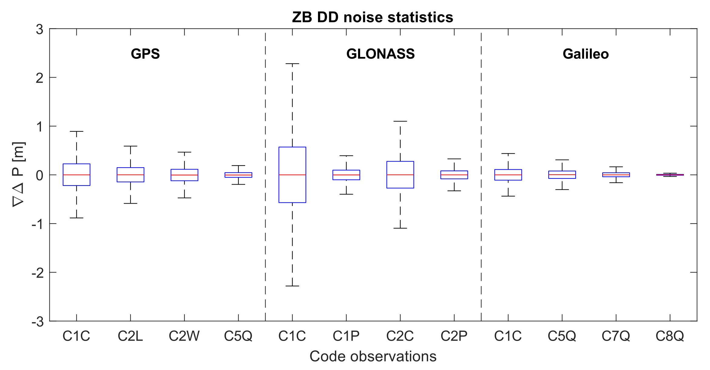
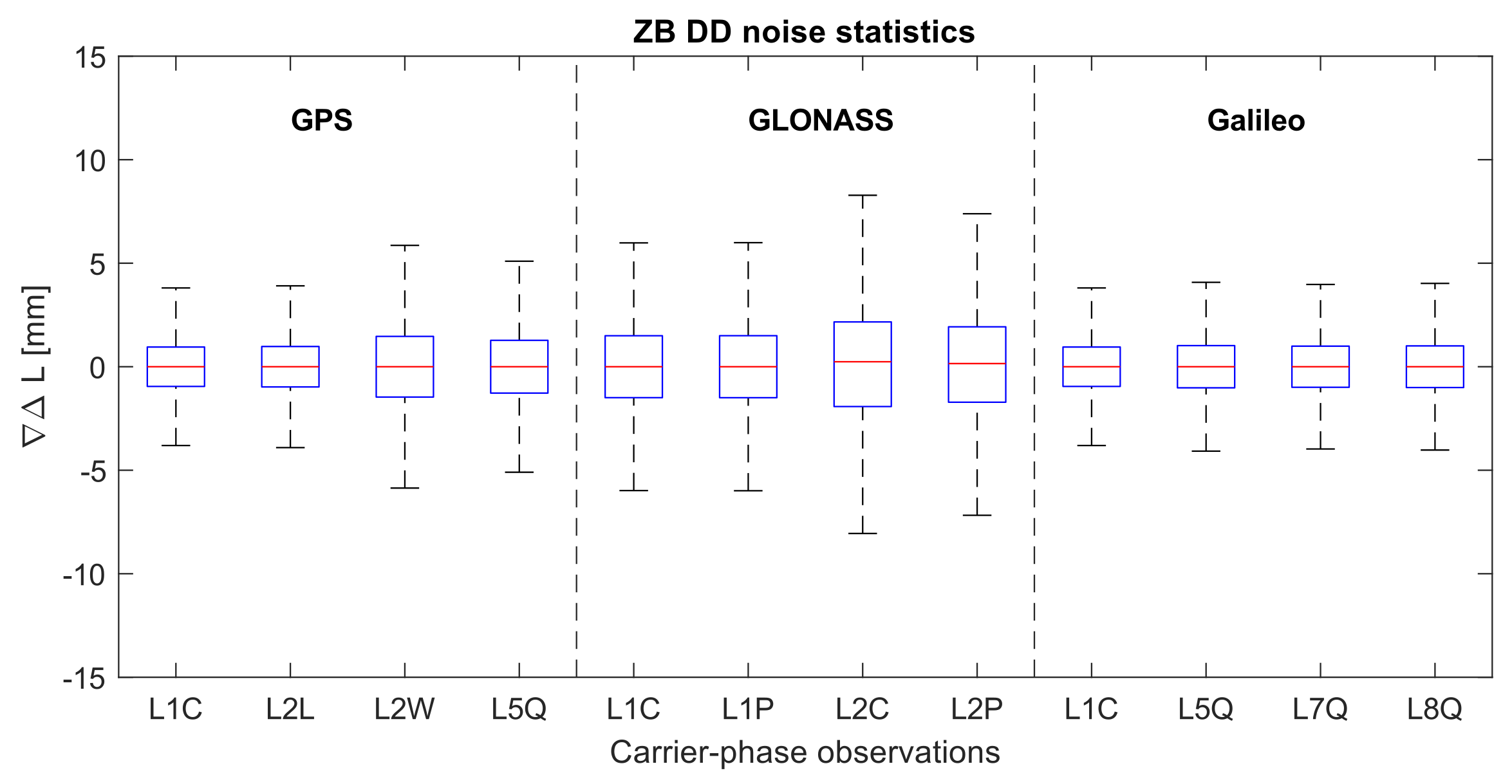
4. Results
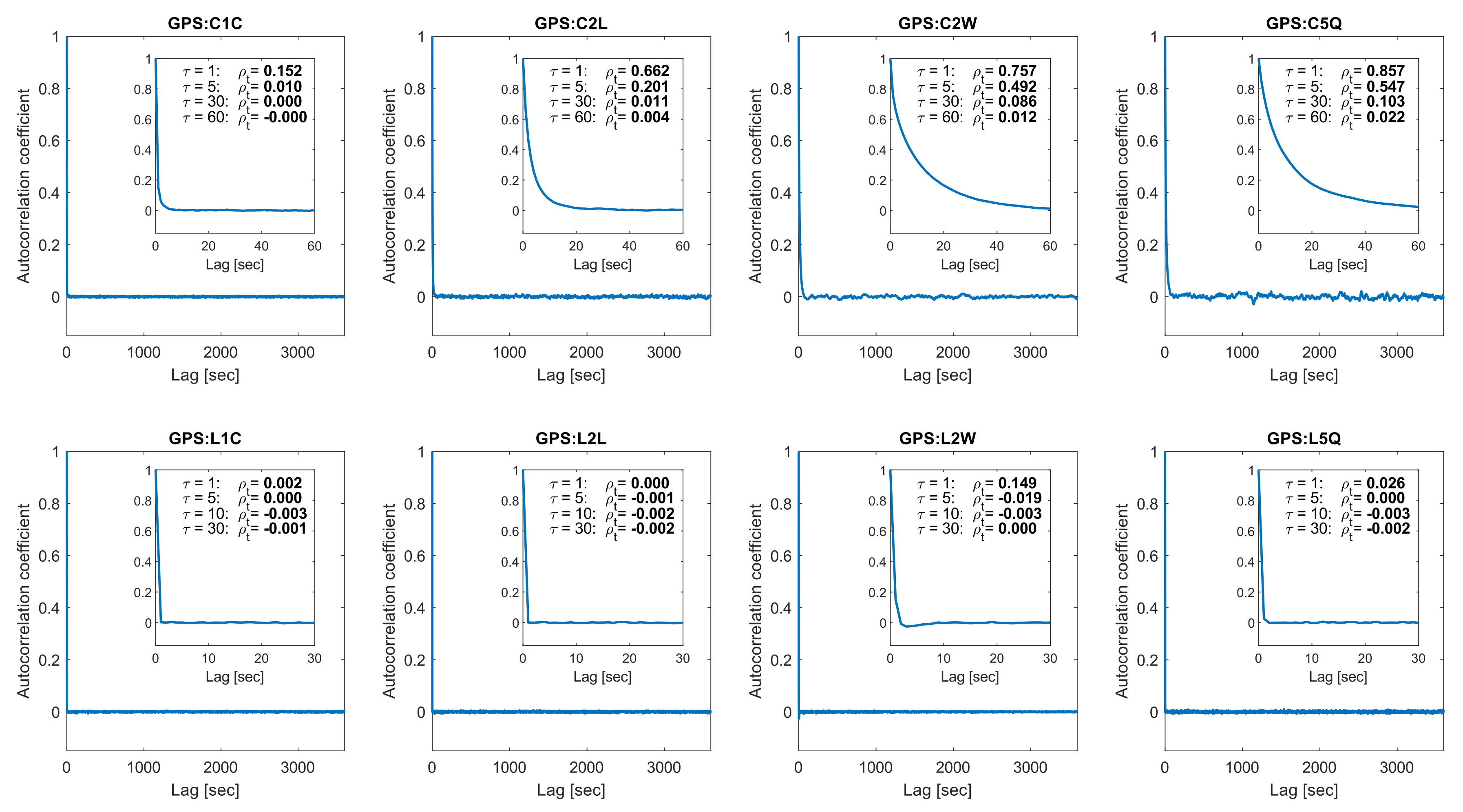
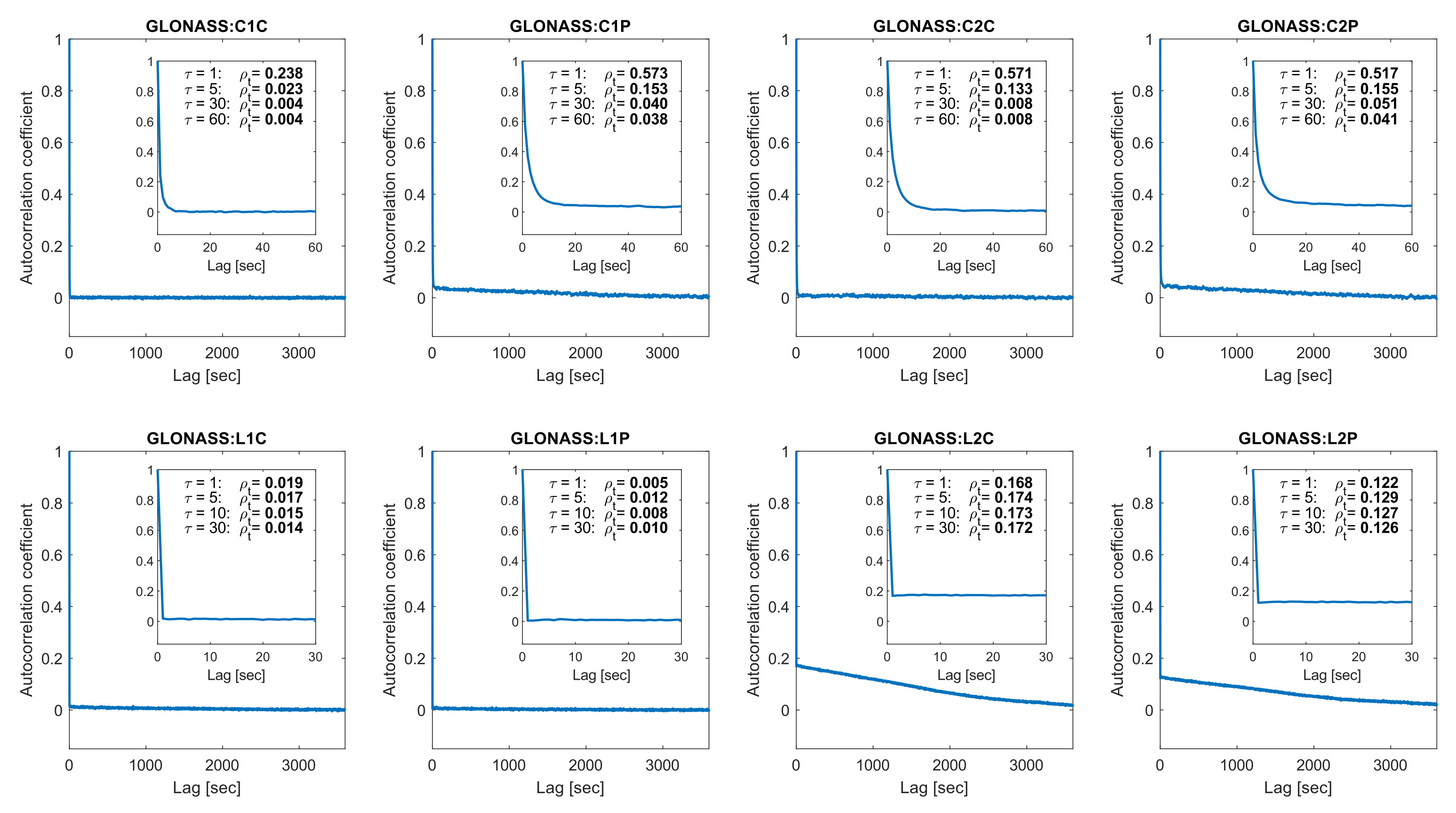
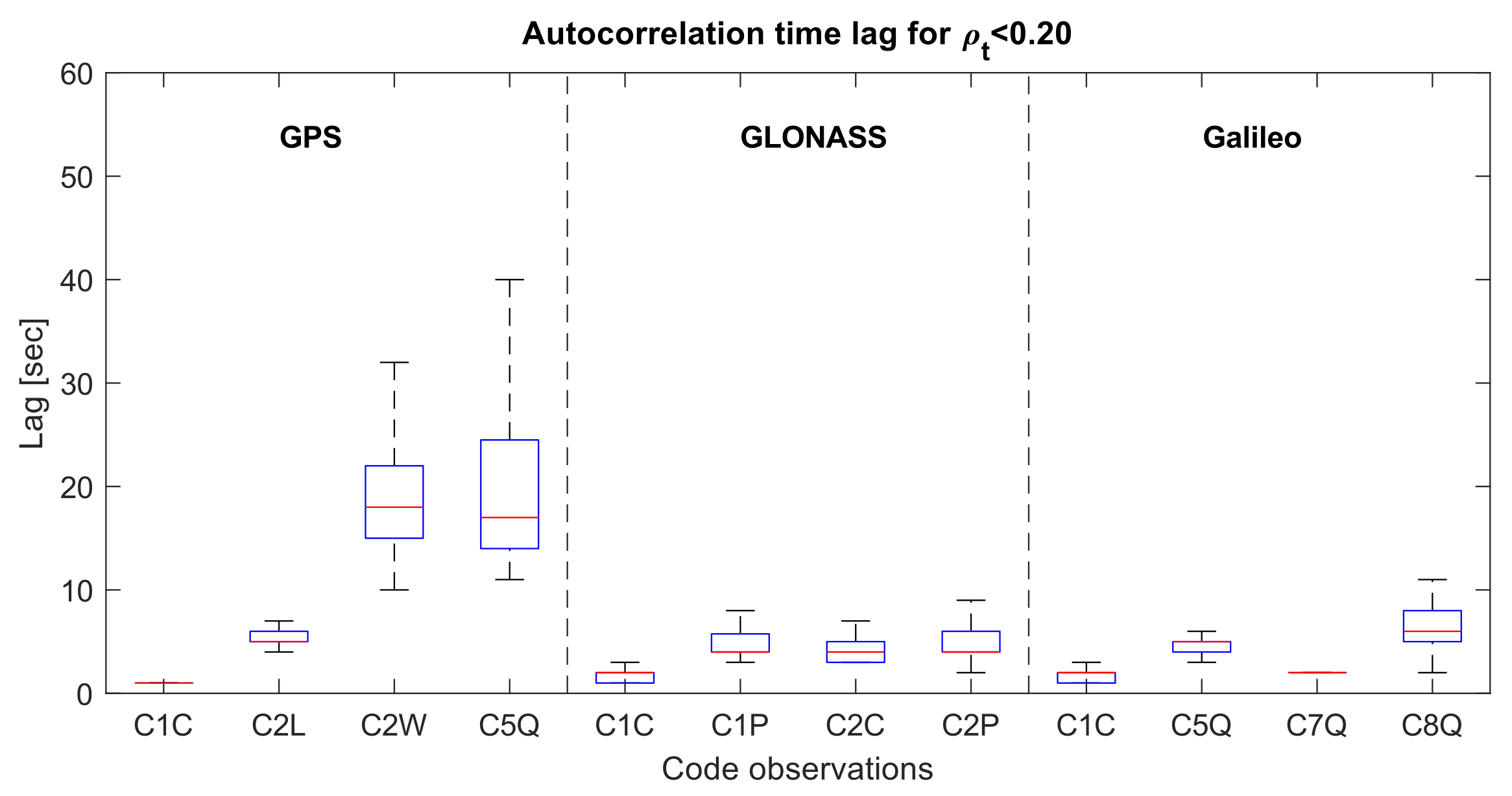
4.1. Autocorrelation Function
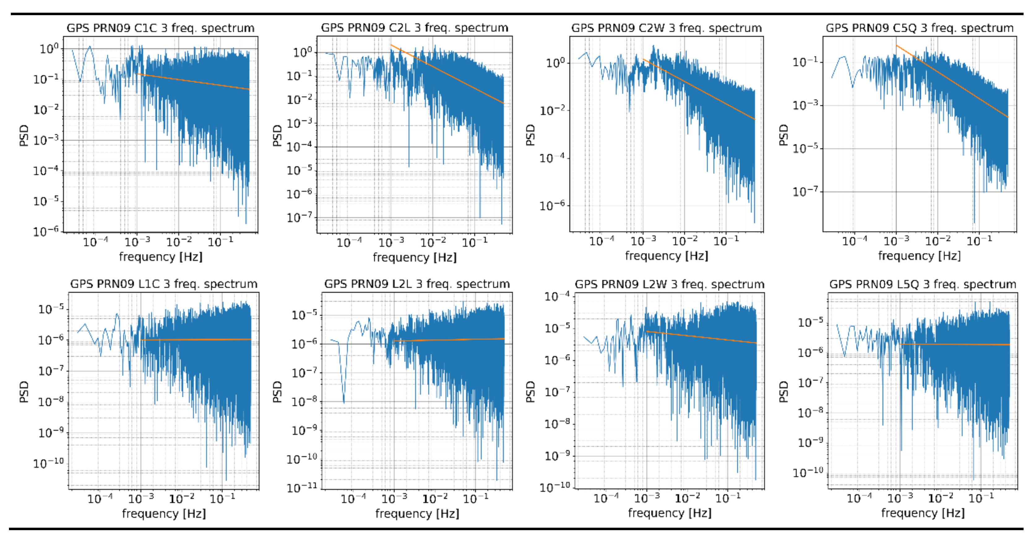
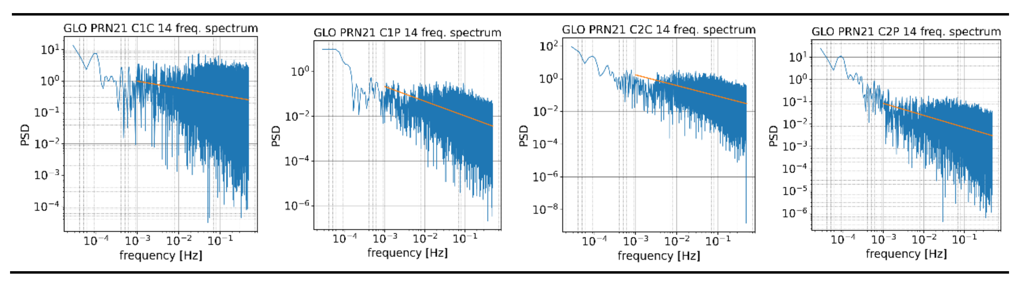
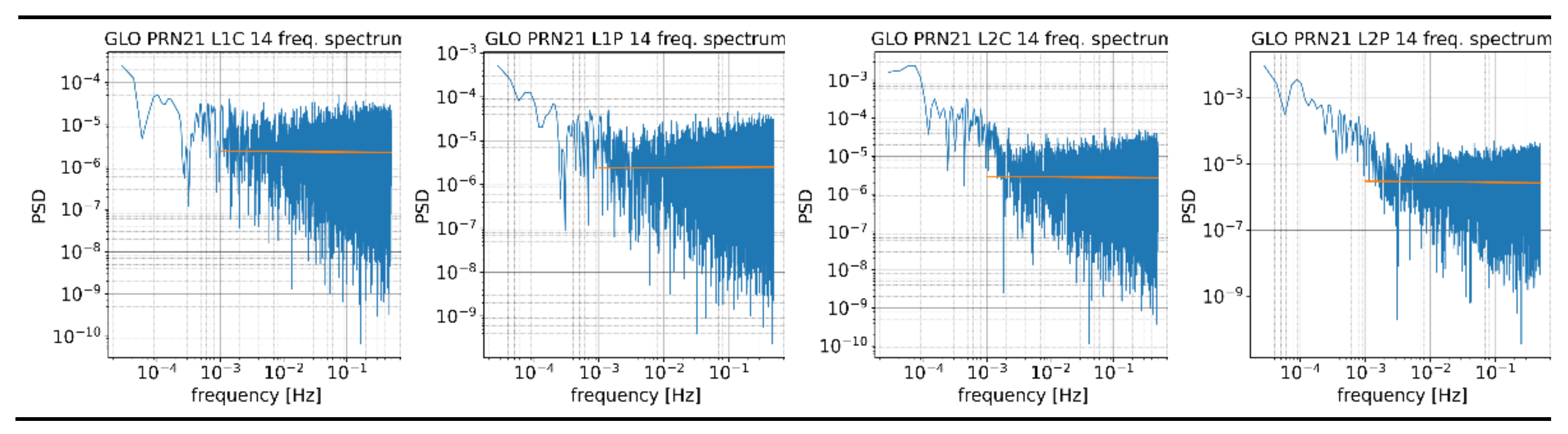
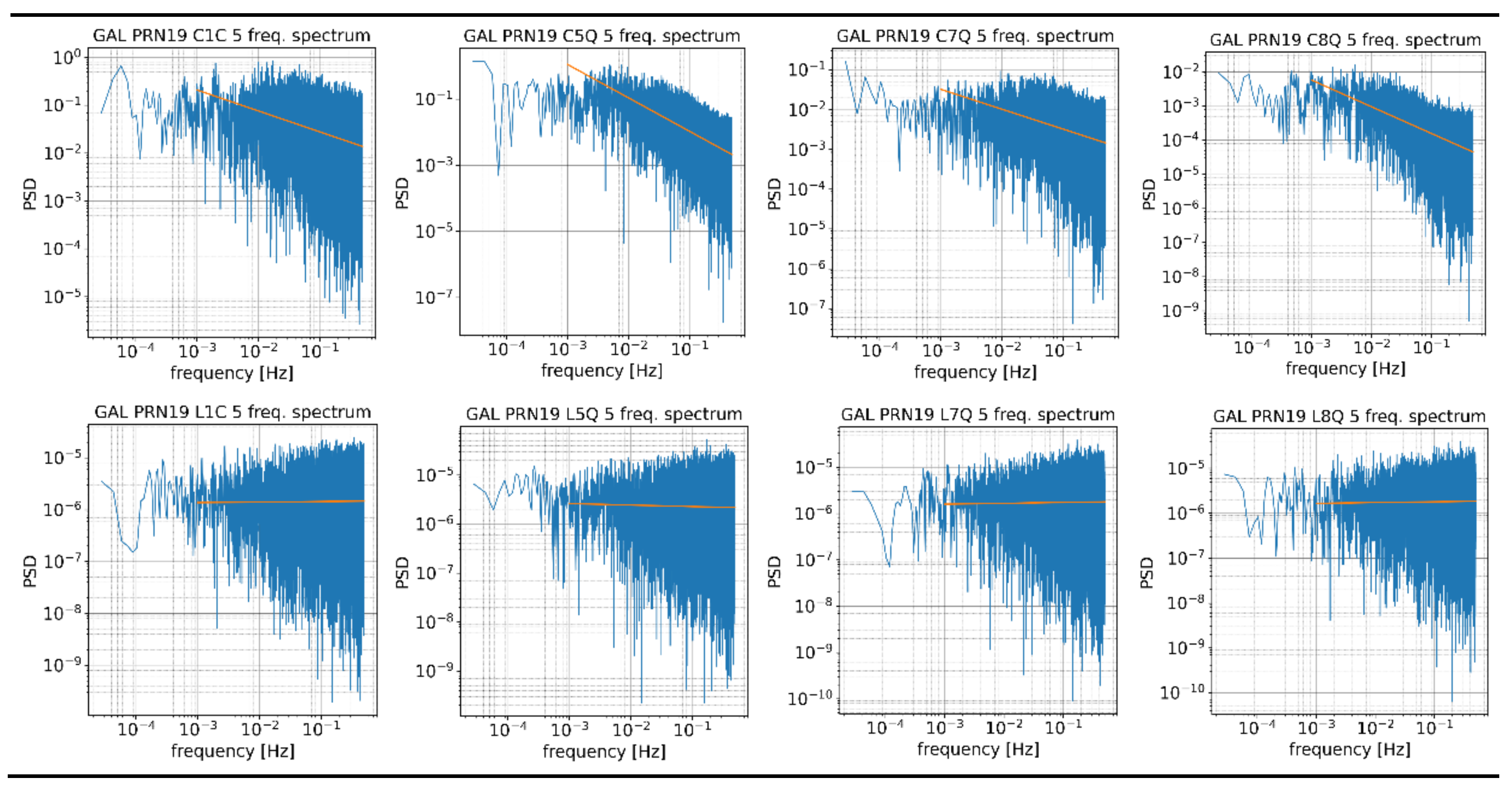
4.2. Spectral Analysis
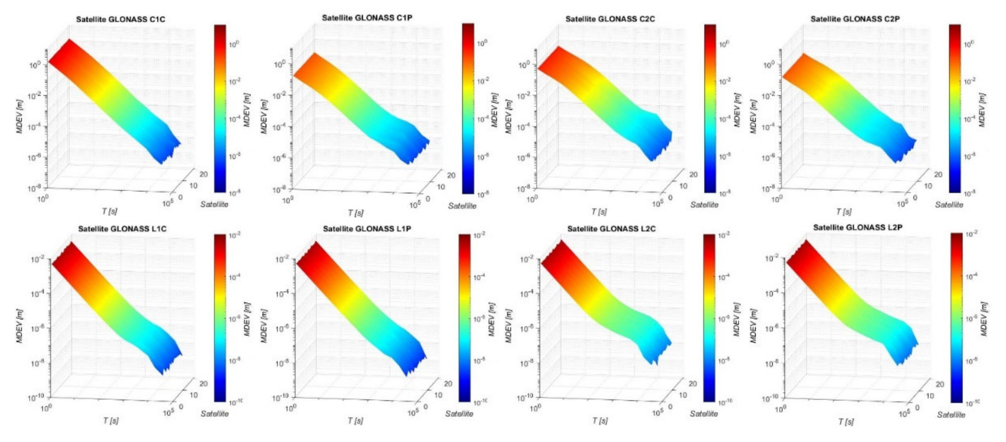
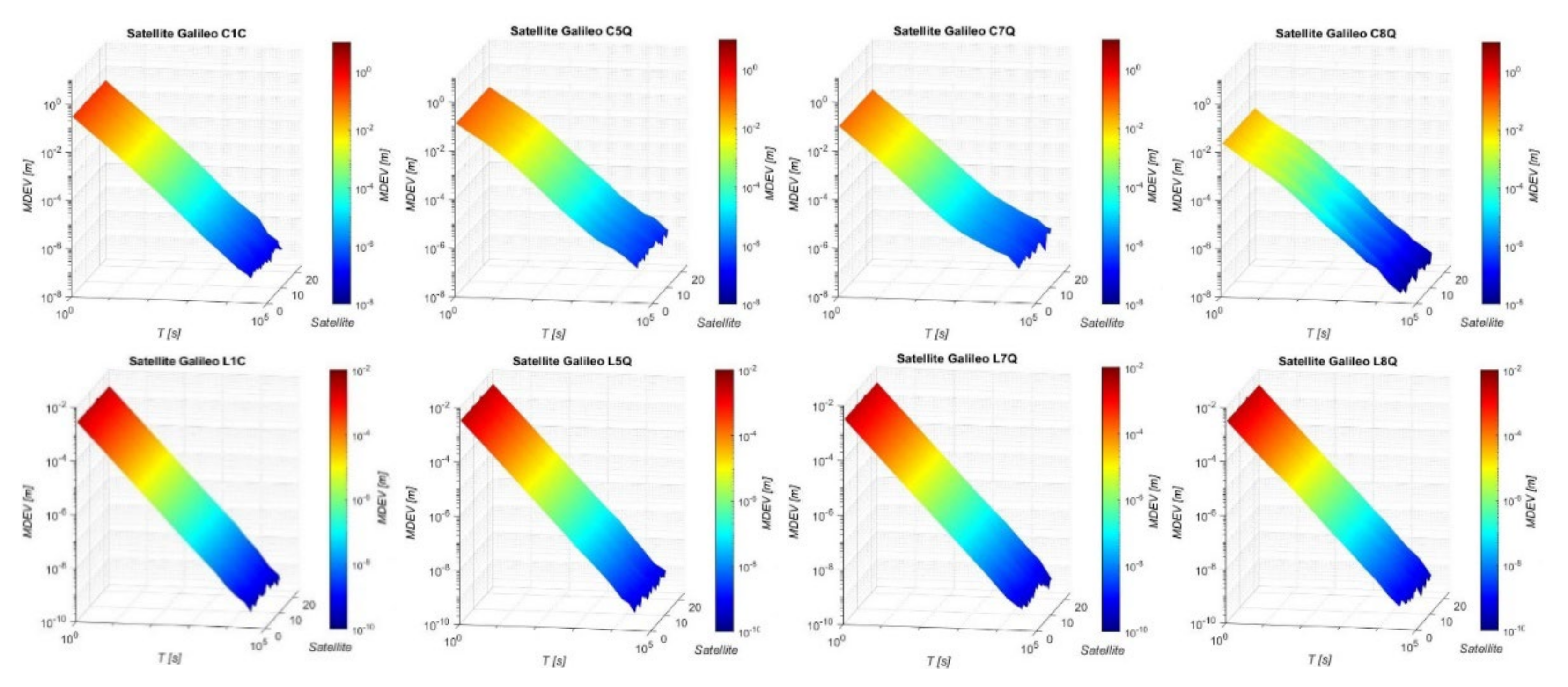
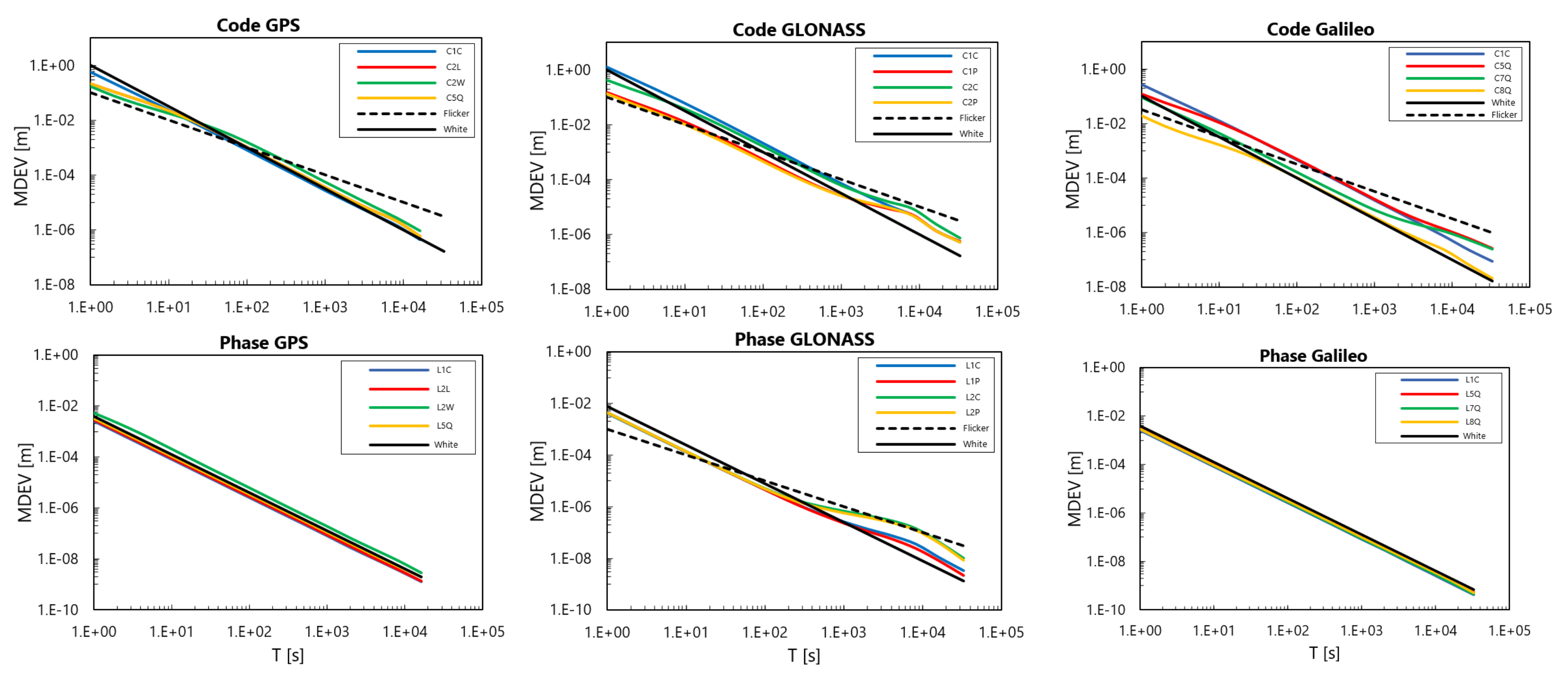
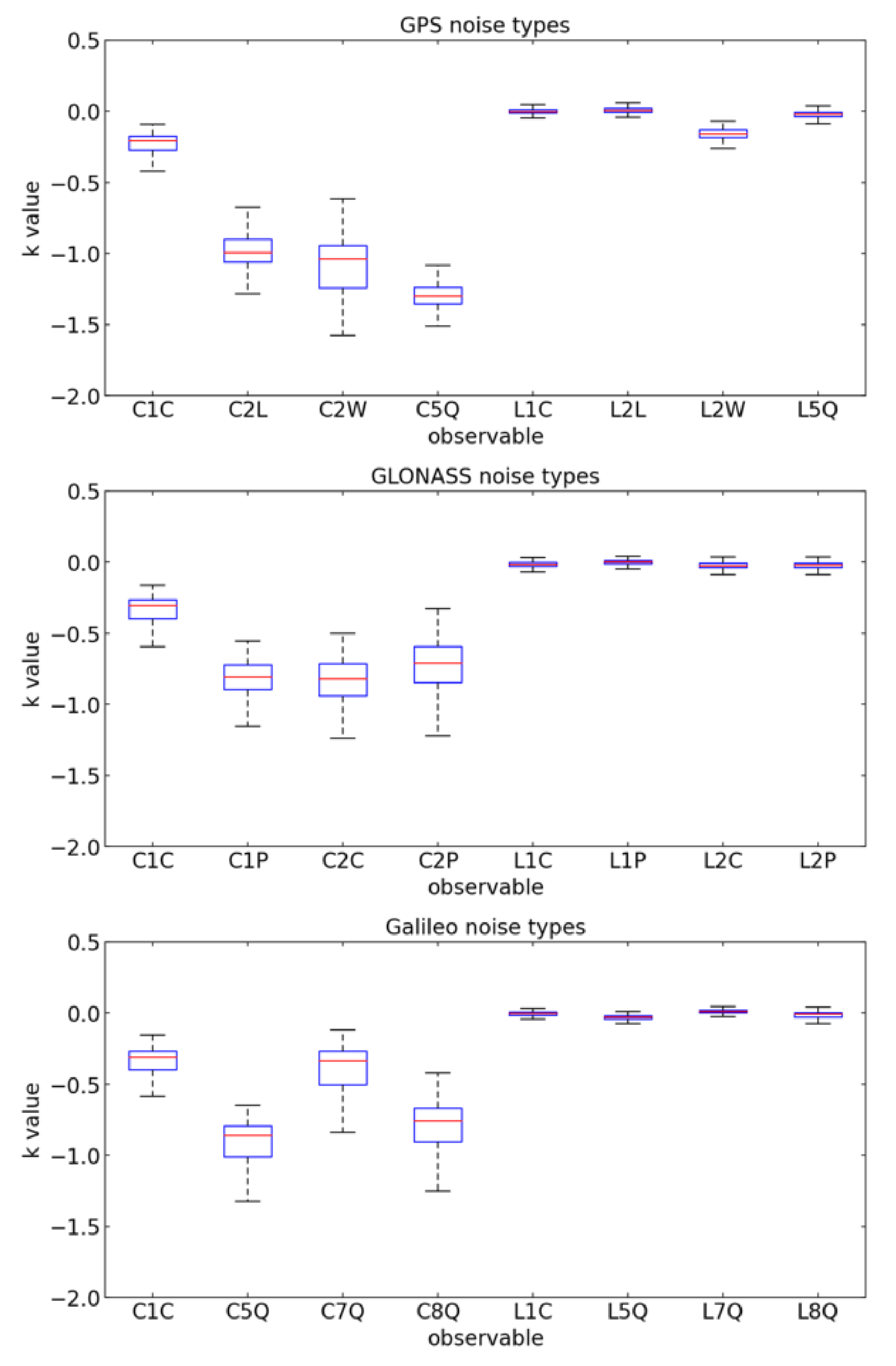
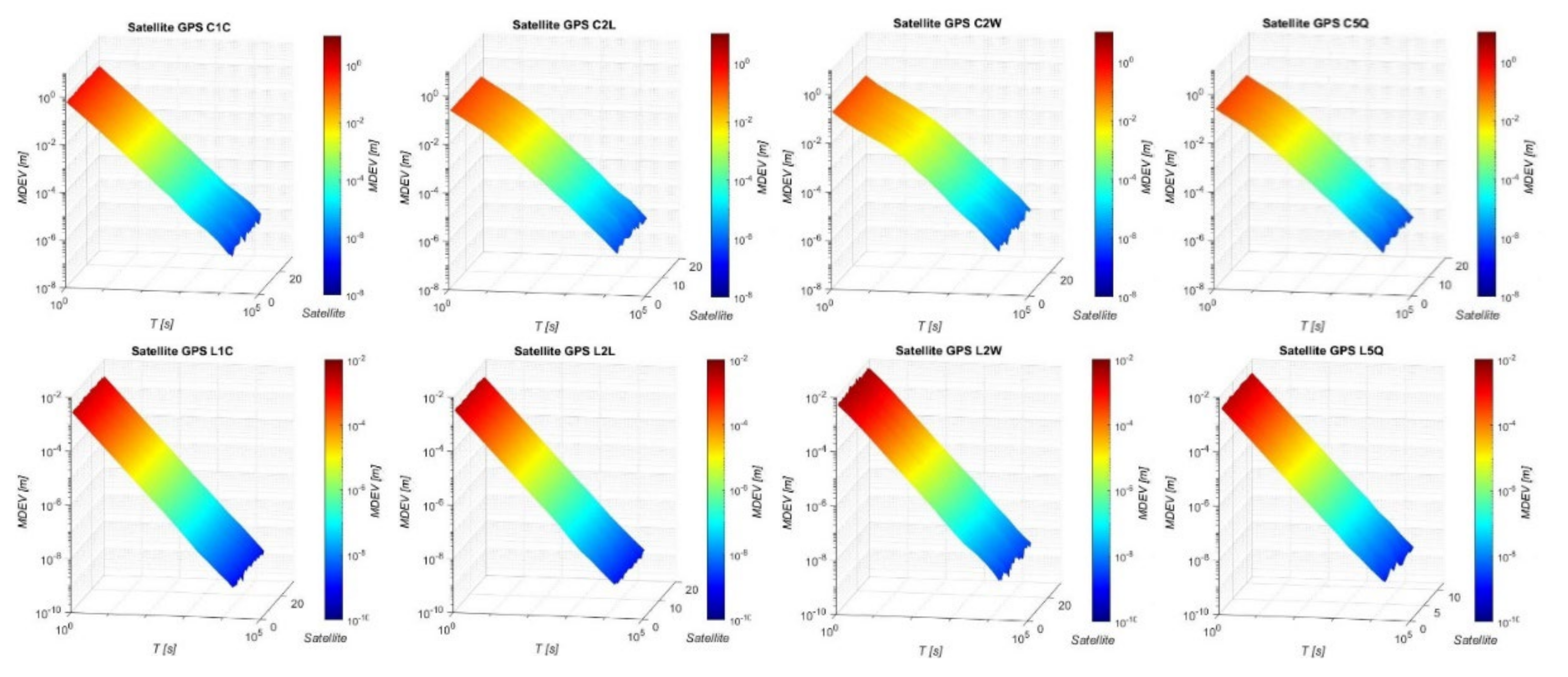
4.3. Allan Variance
5. Discussion and Conclusions
Author Contributions
Funding
Institutional Review Board Statement
Informed Consent Statement
Data Availability Statement
Conflicts of Interest
References
- Borre, K.; Tiberius, C. Time Series Analysis of GPS Observables. In Proceedings of the 13th International Technical Meeting of the Satellite Division of The Institute of Navigation ION GP, Salt Lake City, UT, USA, 19–22 September 2000; pp. 1885–1894. [Google Scholar]
- Zangenehnejad, F.; Gao, Y. GNSS smartphones positioning: Advances, challenges, opportunities, and future perspectives. Satell. Navig. 2021, 2, 24. [Google Scholar] [CrossRef] [PubMed]
- Paziewski, J.; Sieradzki, R.; Baryla, R. Signal characterization and assessment of code GNSS positioning with low-power consumption smartphones. GPS Solut. 2019, 23, 98. [Google Scholar] [CrossRef] [Green Version]
- Luo, Y.; Li, J.; Yu, C.; Xu, B.; Li, Y.; Hsu, L.T.; El-Sheimy, N. Research on Time-Correlated Errors Using Allan Variance in a Kalman Filter Applicable to Vector-Tracking-Based GNSS Software-Defined Receiver for Autonomous Ground Vehicle Navigation. Remote Sens. 2019, 11, 1026. [Google Scholar] [CrossRef] [Green Version]
- Wang, D.; Dong, Y.; Li, Q.; Li, Z.; Wu, J. Using Allan variance to improve stochastic modeling for accurate GNSS/INS integrated navigation. GPS Solut. 2018, 22, 53. [Google Scholar] [CrossRef]
- Wang, J. Stochastic Assessment of the GPS Measurements for Precise Positioning. In Proceedings of the 11th International Technical Meeting of the Satellite Division of The Institute of Navigation (ION GPS 1998), Nashville, TN, USA, 15–18 September 1998; pp. 81–89. [Google Scholar]
- Howind, J.; Kutterer, H.; Heck, B. Impact of temporal correlations on GPS-derived relative point positions. J. Geod. 1999, 73, 246–258. [Google Scholar] [CrossRef]
- Bona, P. Precision, Cross Correlation, and Time Correlation of GPS Phase and Code Observations. GPS Solut. 2000, 4, 3–13. [Google Scholar] [CrossRef]
- Teunissen, P.J.G.; Jonkman, N.F.; Tiberius, C.C.J.M. Weighting GPS Dual Frequency Observations: Bearing the Cross of Cross-Correlation. GPS Solut. 1998, 2, 28–37. [Google Scholar] [CrossRef] [Green Version]
- Schön, S.; Brunner, F.K. A proposal for modelling physical correlations of GPS phase observations. J. Geod. 2008, 82, 601–612. [Google Scholar] [CrossRef]
- Foucras, M.; Leclère, J.; Botteron, C.; Julien, O.; Macabiau, C.; Farine, P.A.; Ekambi, B. Study on the cross-correlation of GNSS signals and typical approximations. GPS Solut. 2017, 21, 293–306. [Google Scholar] [CrossRef]
- Hou, P.; Zhang, B.; Yuan, Y. Analysis of the stochastic characteristics of GPS/BDS/Galileo multi-frequency observables with different types of receivers. J. Spat. Sci. 2021, 66, 49–73. [Google Scholar] [CrossRef]
- Prochniewicz, D.; Wezka, K.; Kozuchowska, J. Empirical stochastic model of multi-GNSS measurements. Sensors 2021, 21, 4566. [Google Scholar] [CrossRef]
- Eueler, H.J.; Goad, C.C. On optimal filtering of GPS dual frequency observations without using orbit information. Bull. Géodésique 1991, 65, 130–143. [Google Scholar] [CrossRef]
- Xiang Jin, X.; de Jong, C.D. Relationship between Satellite Elevation and Precision of GPS Code Observations. J. Navig. 1996, 49, 253–265. [Google Scholar] [CrossRef]
- Li, B. Stochastic modeling of triple-frequency BeiDou signals: Estimation, assessment and impact analysis. J. Geod. 2016, 90, 593–610. [Google Scholar] [CrossRef]
- Gianniou, M.; Groten, E. An Advanced Real-Time Algorithm for Code and Phase DGPS. In Proceedings of the DSNS’96 Conference, St. Petersburg, Russia, 20–24 May 1996. [Google Scholar]
- Luo, X.; Mayer, M.; Heck, B. Improving the Stochastic Model of GNSS Observations by Means of SNR-based Weighting. In Observing our Changing Earth; Springer: Berlin/Heidelberg, Germany, 2009; pp. 725–734. [Google Scholar]
- Talbot, N. Optimal weighting of GPS carrier phase observations based on the signal-to-noise ratio. In Proceedings of the International Symposia on Global Positioning Systems, Queensland, Australia, 17–19 October 1988. [Google Scholar]
- Hartinger, H.; Brunner, F.K. Variances of GPS Phase Observations: The SIGMA-ε Model. GPS Solut. 1999, 2, 35–43. [Google Scholar] [CrossRef]
- Andreas Wieser, F.K.B. An extended weight model for GPS phase observations. Earth Planets Sp. 2000, 52, 777–782. [Google Scholar] [CrossRef] [Green Version]
- Aquino, M.; Monico, J.F.G.; Dodson, A.H.; Marques, H.; De Franceschi, G.; Alfonsi, L.; Romano, V.; Andreotti, M. Improving the GNSS positioning stochastic model in the presence of ionospheric scintillation. J. Geod. 2009, 83, 953–966. [Google Scholar] [CrossRef]
- da Silva, H.A.; de Oliveira Camargo, P.; Galera Monico, J.F.; Aquino, M.; Marques, H.A.; De Franceschi, G.; Dodson, A. Stochastic modelling considering ionospheric scintillation effects on GNSS relative and point positioning. Adv. Sp. Res. 2010, 45, 1113–1121. [Google Scholar] [CrossRef]
- Seepersad, G.; Bisnath, S. Reduction of precise point positioning convergence period. In Proceedings of the 25th International Technical Meeting of the Satellite Division of the Institute of Navigation 2012, ION GNSS 2012, Nashville, TN, USA, 17–21 September 2012; Volume 5, pp. 3742–3752. [Google Scholar]
- Luo, X. GPS Stochastic Modelling-Signal Quality Measures and ARMA Processes; Springer Science & Business Media: Berlin/Heidelberg, Germany, 2013. [Google Scholar]
- El-Rabbany, A. The Effect of Physical Correlations on the Ambiguity Resolution and Accuracy Estimation in GPS Differential Positioning; University of New Brunswick: Fredericton, NB, Canada, 1994. [Google Scholar]
- Tiberius, C.; Jonkman, N.; Kenselaar, F. The stochastics of GPS observables. GPS World 1999, 10, 49–54. [Google Scholar]
- Li, B.; Shen, Y.; Xu, P. Assessment of stochastic models for GPS measurements with different types of receivers. Sci. Bull. 2008, 53, 3219–3225. [Google Scholar] [CrossRef] [Green Version]
- Pilgram, B.; Kaplan, D.T. A comparison of estimators for noise. Phys. D Nonlinear Phenom. 1998, 114, 108–122. [Google Scholar] [CrossRef]
- Levitin, D.J.; Chordia, P.; Menon, V. Musical rhythm spectra from Bach to Joplin obey a 1/f power law. Proc. Natl. Acad. Sci. USA 2012, 109, 3716–3720. [Google Scholar] [CrossRef] [PubMed] [Green Version]
- Gabaix, X. Power Laws in Economics and Finance; Annual Review of Economics: Cambridge, MA, USA, 2008. [Google Scholar]
- Bos, M.S.; Fernandes, R.M.S.; Williams, S.D.P.; Bastos, L. Fast error analysis of continuous GPS observations. J. Geod. 2008, 82, 157–166. [Google Scholar] [CrossRef] [Green Version]
- Chen, X.; Peng, C.; Huan, H.; Nian, F.; Yang, B. Measuring the Power Law Phase Noise of an RF Oscillator with a Novel Indirect Quantitative Scheme. Electronics 2019, 8, 767. [Google Scholar] [CrossRef] [Green Version]
- Vaughan, S. A simple test for periodic signals in red noise. Astron. Astrophys. 2005, 431, 391–403. [Google Scholar] [CrossRef]
- Williams, S.D.P.; Bock, Y.; Fang, P.; Jamason, P.; Nikolaidis, R.M. Error analysis of continuous GPS position time series. J. Geophys. Res. 2004, 109, B03412. [Google Scholar] [CrossRef] [Green Version]
- Williams, S.D.P. CATS: GPS coordinate time series analysis software. GPS Solut. 2008, 12, 147–153. [Google Scholar] [CrossRef]
- Lomb, N.R. Least-squares frequency analysis of unequally spaced data. Astrophys. Space Sci. 1976, 39, 447–462. [Google Scholar] [CrossRef]
- Scargle, J.D. Studies in astronomical time series analysis. II-Statistical aspects of spectral analysis of unevenly spaced data. Astrophys. J. 1982, 263, 835. [Google Scholar] [CrossRef]
- Allan, D.W. Statistics of atomic frequency standards. Proc. IEEE 1966, 54, 221–230. [Google Scholar] [CrossRef] [Green Version]
- Hackl, M.; Malservisi, R.; Hugentobler, U.; Jiang, Y. Velocity covariance in the presence of anisotropic time correlated noise and transient events in GPS time series. J. Geodyn. 2013, 72, 36–45. [Google Scholar] [CrossRef]
- Malkin, Z. Application of the Allan Variance to Time Series Analysis in Astrometry and Geodesy: A Review. IEEE Trans. Ultrason. Ferroelectr. Freq. Control 2016, 63, 582–589. [Google Scholar] [CrossRef] [Green Version]
- Hefty, J.; Igondová, M.; Hrcka, M. Contribution of Gps Permanent Stations in Central Europe to Regional Geo-Kinematical Investigations. Acta Geodyn. Geomater. 2005, 2, 75–86. [Google Scholar]
- Le Bail, K. Etude Statistique de la Stabileté des Stations de Géodésie Spatiale, Application à DORIS; Observatoire de Paris: Paris, France, 2004. [Google Scholar]
- Howe, D.A.; Allan, D.U.; Barnes, J.A. Properties of Signal Sources and Measurement Methods. In Proceedings of the Thirty Fifth Annual Frequency Control Symposium, Philadelphia, PA, USA, 27–29 May 1981; pp. 669–716. [Google Scholar]
- Le Bail, K. Estimating the noise in space-geodetic positioning: The case of DORIS. J. Geod. 2006, 80, 541–565. [Google Scholar] [CrossRef]
- Khelifa, S.; Kahlouche, S.; Belbachir, M.F. Analysis of position time series of GPS-DORIS co-located stations. Int. J. Appl. Earth Obs. Geoinf. 2012, 20, 67–76. [Google Scholar] [CrossRef]
- de Bakker, P.F.; van der Marel, H.; Tiberius, C.C.J.M. Geometry-free undifferenced, single and double differenced analysis of single frequency GPS, EGNOS and GIOVE-A/B measurements. GPS Solut. 2009, 13, 305–314. [Google Scholar] [CrossRef] [Green Version]
- Gourevitch, S. Innovation: Measuring GPS receiver performance—A new approach. GPS World 1996, 7, 56–62. [Google Scholar]
- Amiri-Simkooei, A.R.; Tiberius, C.C.J.M.; Teunissen, P.J.G. Assessment of noise in GPS coordinate time series: Methodology and results. J. Geophys. Res. Solid Earth 2007, 112, 1–19. [Google Scholar] [CrossRef] [Green Version]
- Petovello, M.G.; Lachapelle, G. Estimation of Clock Stability Using GPS. GPS Solut. 2000, 4, 21–33. [Google Scholar] [CrossRef]
- Jia, X.; Zeng, T.; Ruan, R.; Mao, Y.; Xiao, G. Atomic clock performance assessment of BeiDou-3 basic system with the noise analysis of orbit determination and time synchronization. Remote Sens. 2019, 11, 2895. [Google Scholar] [CrossRef] [Green Version]
- Wang, G.; Liu, L.; Xu, A.; Pan, F.; Cai, Z.; Xiao, S.; Tu, Y.; Li, Z. On the capabilities of the inaction method for extracting the periodic components from GPS clock data. GPS Solut. 2018, 22, 1–14. [Google Scholar] [CrossRef] [Green Version]
- Riley, W.J. Handbook of Frequency Stability Analysis; National Institute of Standards and Technology: Gaithersburg, MD, USA, 2008; Volume 31, ISBN 3019753058. [Google Scholar]
- IGS RINEX WG, RTCM-SC104. RINEX—The Receiver Independent EXchange Format. Version 3.04. 2018. Available online: http://acc.igs.org/misc/rinex304.pdf (accessed on 1 December 2021).
- Al-shaery, A.; Lim, S.; Rizos, C. Challenges of Seamless Multi-GNSS. In Proceedings of the IAIN Congress, Cairo, Egypt, 1–3 October 2012; pp. 1–20. [Google Scholar]


| System/ Observation Type | L1 | L2 | L5 |
|---|---|---|---|
| GPS | C1C/L1C | C2L/L2L C2W/L2W | C5Q/L2Q |
| GLONASS | C1C/L1C C1P/L1P | C2C/L2C C2P/L2P | |
| Galileo | C1C/L1C | C5Q/L5Q C7Q/L7Q C8Q/L8Q |
| System/Observation Type | Code (m) | Phase (mm) | |||
|---|---|---|---|---|---|
| Mean | Std. | Mean | Std. | ||
| GPS | 1C | 0.002 | ±0.370 | 0.00 | ±1.50 |
| 2L | −0.001 | ±0.243 | 0.00 | ±1.69 | |
| 2W | −0.002 | ±0.229 | 0.00 | ±3.41 | |
| 5Q | −0.001 | ±0.095 | 0.00 | ±1.95 | |
| GLONASS | 1C | 0.001 | ±0.891 | 0.00 | ±2.41 |
| 1P | −0.002 | ±0.151 | 0.00 | ±2.50 | |
| 2C | 0.002 | ±0.444 | 0.03 | ±3.03 | |
| 2P | −0.001 | ±0.133 | 0.01 | ±2.92 | |
| Galileo | 1C | 0.000 | ±0.182 | 0.00 | ±1.47 |
| 5Q | 0.003 | ±0.121 | 0.00 | ±1.81 | |
| 7Q | 0.000 | ±0.064 | 0.00 | ±1.66 | |
| 8Q | 0.000 | ±0.020 | 0.00 | ±1.67 | |
| System/ Observation Type | Time Lag [sec] | ||
|---|---|---|---|
| Code | Phase | ||
| GPS | 1C | ≤1 | ≤1 |
| 2L | 5 | ≤1 | |
| 2W | 18 | ≤1 | |
| 5Q | 17 | ≤1 | |
| GLONASS | 1C | 2 | ≤1 |
| 1P | 4 | ≤1 | |
| 2C | 4 | ≤1 | |
| 2P | 4 | ≤1 | |
| Galileo | 1C | 2 | ≤1 |
| 5Q | 5 | ≤1 | |
| 7Q | 2 | ≤1 | |
| 8Q | 6 | ≤1 | |
| System/ Observation Type | Number of Arcs | Code | Phase | |||
|---|---|---|---|---|---|---|
| Median | std dev | Median | std dev | |||
| GPS | 1C | 429 | −0.2 | 0.12 | 0.0 | 0.03 |
| 2L | 242 | −1.0 | 0.12 | 0.0 | 0.03 | |
| 2W | 401 | −1.0 | 0.19 | −0.2 | 0.04 | |
| 5Q | 151 | −1.3 | 0.14 | 0.0 | 0.04 | |
| GLONASS | 1C | 321 | −0.3 | 0.11 | 0.0 | 0.02 |
| 1P | 317 | −0.8 | 0.13 | 0.0 | 0.02 | |
| 2C | 321 | −0.8 | 0.16 | 0.0 | 0.03 | |
| 2P | 321 | −0.7 | 0.19 | 0.0 | 0.03 | |
| Galileo | 1C | 268 | −0.3 | 0.11 | 0.0 | 0.02 |
| 5Q | 268 | −0.9 | 0.14 | 0.0 | 0.02 | |
| 7Q | 268 | −0.3 | 0.18 | 0.0 | 0.02 | |
| 8Q | 268 | −0.8 | 0.23 | 0.0 | 0.06 | |
Publisher’s Note: MDPI stays neutral with regard to jurisdictional claims in published maps and institutional affiliations. |
© 2022 by the authors. Licensee MDPI, Basel, Switzerland. This article is an open access article distributed under the terms and conditions of the Creative Commons Attribution (CC BY) license (https://creativecommons.org/licenses/by/4.0/).
Share and Cite
Prochniewicz, D.; Kudrys, J.; Maciuk, K. Noises in Double-Differenced GNSS Observations. Energies 2022, 15, 1668. https://doi.org/10.3390/en15051668
Prochniewicz D, Kudrys J, Maciuk K. Noises in Double-Differenced GNSS Observations. Energies. 2022; 15(5):1668. https://doi.org/10.3390/en15051668
Chicago/Turabian StyleProchniewicz, Dominik, Jacek Kudrys, and Kamil Maciuk. 2022. "Noises in Double-Differenced GNSS Observations" Energies 15, no. 5: 1668. https://doi.org/10.3390/en15051668
APA StyleProchniewicz, D., Kudrys, J., & Maciuk, K. (2022). Noises in Double-Differenced GNSS Observations. Energies, 15(5), 1668. https://doi.org/10.3390/en15051668