Comparison of Flame Propagation Statistics Based on Direct Numerical Simulation of Simple and Detailed Chemistry. Part 2: Influence of Choice of Reaction Progress Variable

Abstract

Flame propagation statistics for turbulent, statistically planar premixed flames obtained from 3D Direct Numerical Simulations using both simple and detailed chemistry have been evaluated and compared to each other. To achieve this, a new database has been established encompassing five different conditions on the turbulent combustion regime diagram, using nearly identical numerical methods and the same initial and boundary conditions. The discussion includes interdependencies of displacement speed and its individual components as well as surface density function (i.e., magnitude of the reaction progress variable) with tangential strain rate and curvature. For the analysis of detailed chemistry Direct Numerical Simulation data, three different definitions of reaction progress variable, based on ${\mathrm{CH}}_4,{\mathrm{H}}_2\mathrm{O}$ and ${\mathrm{O}}_2$ mass fractions will be used. While the displacement speed statistics remain qualitatively and to a large extent quantitatively similar for simple chemistry and detailed chemistry, there are pronounced differences for its individual contributions which to a large extent depend on the definition of reaction progress variable as well as on the chosen isosurface level. It is concluded that, while detailed chemistry simulations provide more detailed information about the flame structure, the choice of the reaction progress variable definition and the choice of the resulting isosurface give rise to considerable uncertainty in the interpretation of displacement speed statistics, sometimes even showing opposing trends. Simple chemistry simulations are shown to provide (a) the global flame propagation statistics which are qualitatively similar to the corresponding results from detailed chemistry simulations, (b) remove the uncertainties with respect to the choice of reaction progress variable, and (c) are more straightforward to compare with theoretical analysis or model assumptions that are mostly based on simple chemistry assumptions.

1. Introduction

The use of fossil resources for the supply of primary energy leads to increasing concerns about emissions and their environmental, and health impact [1]. However, the challenges laid out by the Paris Agreement are daunting [2] and the time scales to phase out the existing infrastructure are substantial [1]. Therefore, combustion remains a topic of considerable importance and Direct Numerical Simulations (DNS) offer valuable insights into the physical and thermochemical phenomena, as reviewed for the early DNS work by Poinsot et al. [3], and more recently by Chen [4]. The ever-growing computing power is an enabler for two trends in recent combustion DNS research: Firstly (not discussed here but underlining the importance of combustion DNS), the availability of high-fidelity datasets has given a significant boost to the development of turbulence and combustion models using machine learning methods [5] and secondly detailed chemical kinetic models for larger and larger hydrocarbon and oxygenated hydrocarbon molecules are being produced [6]. While practical fuels for transportation often contain thousands of distinct chemical compounds [7], there is also an increasing interest in simple fuels such as hydrogen [8,9] or syngas [10,11] that could play an important role during the transition of the fuel landscape. Their main components such as ${\mathrm{H}}_2, \mathrm{CO}$ and ${\mathrm{CH}}_4$ are conceptually at the base of detailed chemical reaction mechanisms that describe much more complex hydrocarbon combustion [12]. Early work on two-dimensional fully resolved simulations of methane-air flames has been reported for example in [13,14,15]. Peters et al. [13] focused on the three different mechanisms arising from the chemical reaction, flame normal diffusion, and flame curvature, which dictate the statistical behavior of flame displacement speed. A similar analysis was performed by Echekki and Chen [14] to identify the contributions of curvature to the displacement speed by using the governing transport equation for the deficient reactant. Chen and Im [15] analysed the curvature stretch correlation indicating two distinct branches, one for positive and one for negative displacement speeds. The authors also indicated the large importance of curvature stretch which results in a non-linear flame speed correlation with stretch rate. Methane flames in three dimensions have been discussed by Bell et al. [16].

The complexity for parameterising chemical kinetics, even for simple fuels, ranges from a few species and reactions [17] up to hundreds of species and thousands of reactions [18]. Such mechanisms often become unmanageable for combustion DNS in three dimensions, and the increased complexity underlines the importance of accurate thermodynamic parameters for all species together with collision efficiencies of different third bodies involved in pressure-dependent reactions [6]. While detailed chemical mechanisms provide a wealth of information about the flame structure, they also have disadvantages in the context of analysis, and modelling turbulence–chemistry interaction. The choice of reaction progress variable definition together with the value of a suitable isolevel gives rise to uncertainty in the interpretation of results and it becomes more difficult to compare with theoretical predictions or models which are often based on simple chemistry assumptions. Klein et al. [19] discussed the modelling of turbulent scalar fluxes for different species in hydrogen air flames. The statistics of the turbulent scalar flux transport equation [20] and the flame surface density transport equation [21] revealed remarkable differences when performed for different major species. Finally, the effect of choosing different species on the determination of flame area has been analysed in [22].

In the following discussion, calculations using one irreversible reaction will be referred to as simple chemistry (SC) simulations, while calculations using a detailed chemical mechanism with detailed transport will be abbreviated as detailed chemistry (DC) simulations.

It becomes clear from the foregoing discussion that it is not straightforward to identify one, correct physical system representation for combustion DNS and it should be self-evident, that the methods chosen for the scientific analysis should be commensurate with the requirements of a specific scientific purpose, as argued in [23] because high-performance computing is itself responsible for non-negligible carbon emissions [24,25]. Another tradeoff that should be considered is that SC simulations allow for large parametric variations and at least in some respects, it might be possible to extract more physical insight from a larger matrix of simulations compared to a few very detailed DNS runs. The present work focuses on the fluid-dynamic aspects of flame–turbulence interactions and does not deal with emissions or ignition which would, without any doubt, require a more complex treatment of chemical kinetics. Flame propagation statistics in terms of displacement speed and its stretch rate dependence are of fundamental importance in the level-set and Flame Surface Density-based modelling methodologies [26]. The flame stretch, in turn, can be decomposed into tangential strain rate and curvature stretch contributions. The reader is referred to the textbook of Poinsot and Veynante [26] for a general introduction. The definition of displacement speed typically relies on a suitably defined reaction progress variable and the same holds true for mean flame curvature. Moreover, displacement speed statistics are typically taken on a specific isosurface within the flame front, which again requires the definition of a reaction progress variable together with the identification of the isolevel of reaction progress variable. It has been shown in the first part of this work [23] that displacement speed statistics and their interrelation with curvature and tangential strain rate are in very good qualitative and reasonably good quantitative agreement between simple and detailed chemistry DNS. The present work goes into more detail by analysing the individual components of displacement speed as well as the surface density function (i.e., magnitude of the gradient of reaction progress variable) and their interdependencies with curvature and strain. In particular, the influence of the definition of reaction progress variable will be discussed in detail. Different species participating in the chemical reaction are characterised by different individual Lewis numbers and the global Lewis number is known to influence flame propagation statistics. Such analysis has been pioneered by Rutland and Trouvé [27] for generic planar flame simulations showing a pronounced Lewis number dependent correlation between surface curvature and the local flame speed. It was also shown that the local flame structure is altered in curved regions. The effects of Lewis number on strain rate and curvature dependences of displacement speed have been analysed individually by Chakraborty and Cant in references [28] and [29], respectively. In these analyses, once more, statistically planar turbulent premixed flames have been considered and the same holds true for the analysis of the evolution of flame surface density [30] as well as surface density function [31] which are highly relevant quantities for modelling turbulent premixed combustion. While some effects of curvature might be annihilated in a mean sense for statistically planar flames, the mean curvature plays an important role for Lewis number effects on flame speed statistics, as demonstrated by Ozel Erol et al. [32] for spherical flames and by Rasool et al. [33] for Bunsen flames. Because of the Lewis number dependence, it might be expected that displacement speed statistics will be different for reaction progress variable definitions based on different species mass fractions. Hence, the main objectives of the present analysis are:

• To identify the influence of the definition of reaction progress variable on the statistics of flame propagation and its correlations with curvature and strain.
• To compare results from SC and DC simulations in order to provide information to balance their largely different computational costs as well as their value in terms of degree of detail compared to a larger parametric analysis or larger scale separation.

The same DNS database that was used in reference [23] has been used for this analysis. Although detailed discussions on this database and its numerical implementation were provided in [23], some of that information is repeated here for ensuring the self-contained nature of this paper in Section 2. This will be followed by a detailed discussion of the results and finally, conclusions will be drawn.

2. Direct Numerical Simulation Database

Two different compressible high order DNS codes SENGA [34] and SENGA2 [35] have been used for the present analysis which are described in detail in part 1 of this paper [23] together with all the necessary information related to this database. Both codes solve the conservation equations of mass, momentum, energy and species (see [34,35]) which can also be found in the textbook of Poinsot and Veynante [26]. For self-consistency, a short description summarizing the main features is provided here in tabular form for the numerical methods and physical models (see

Table 1. Numerical methods and physical models used for the DC and SC simulations.

	SC–SENGA [34]	DC–SENGA2 [35]
Governing equations	Compressible, non-dimensional form, ideal gas law	Compressible, dimensional form, ideal gas law
Spatial discretization	Tenth order reducing to 2nd order at non-periodic boundaries	Tenth order reducing to 4th order at non-periodic boundaries
Temporal discretization	Third order low-storage Runge-Kutta scheme [36]	Fourth order low storage Runge–Kutta scheme [37]
Chemistry	1-step irreversible, Arrhenius chemistry	Sixteen species and 25 reactions [17]
Thermodynamic properties	Dynamic viscosity, thermal conductivity and density weighted mass diffusivity are constant and independent of temperature. Standard values for Zel’dovich, Prandtl number and ratio of specific heats $(\beta =6.0$$, Pr=0.7$$, \gamma =1.4$). Lewis number and heat release parameter are taken as 1.0 and 6.5, respectively	Individual mass diffusion coefficients are determined by constant Lewis number assumption see Table 3 [17]. Fifth order Chemkin polynomials for temperature dependent properties [38]

) and a schematic diagram of the computational configuration (see

Table 2. Details of computational configuration.

Configuration	Statistically planar turbulent premixed flame in decaying turbulence (see [39] for comparison of different strategies)
Domain size	Uniform cartesian mesh of size $1024\times 512\times 512$
Computational mesh	$3.066 \mathrm{cm}\times 1.530 \mathrm{cm}\times 1.530 \mathrm{cm}$
Boundary Conditions	Periodic in y- and z-direction, x-axis is aligned with the mean flame propagation direction, Navier Stokes Characteristic Boundary Conditions (NSCBC) [40] are used at all non-periodic boundaries
Initial data	Homogeneous isotropic turbulent flow field [41] with superimposed laminar flame data
Resolution	$\Delta x,y,z=3\times {10}^{-5} m$ which resolves the Kolmogorov scale and as well the thermal flame thickness with 13.7 grid points
Duration	Simulations were run for one chemical time scale which corresponds to at least 3 $(2.14$) eddy turn over times for cases A, B, C, E (case D)

) is presented in Figure 1a, and the species Lewis numbers are presented in

Table 3. Lewis numbers of all species [17].

Species	$\mathbf{C}{\mathbf{H}}_{\mathbf{4}}$	${\mathbf{O}}_{\mathbf{2}}$	${\mathbf{H}}_{\mathbf{2}}\mathbf{O}$	$\mathbf{C}{\mathbf{O}}_{\mathbf{2}}$	$\mathbf{H}$	$\mathbf{O}$	$\mathbf{O}\mathbf{H}$	$\mathbf{H}{\mathbf{O}}_{\mathbf{2}}$
$Le$	$0.97$	$1.11$	0.83	$1.39$	$0.18$	$0.70$	$0.73$	$1.10$
Species	$H_{\mathbf{2}}$	$CO$	$H_{\mathbf{2}}{O}_{\mathbf{2}}$	$HCO$	$C{H}_{2}O$	$C{H}_{\mathbf{3}}$	$C{H}_{\mathbf{3}}O$	$N_{\mathbf{2}}$
$Le$	$0.3$0	$1.10$	$1.12$	$1.27$	$1.28$	$1.00$	$1.30$	$1.00$

. Snapshots of the flame contours at the time when statistics are extracted are exemplarily shown for one case only in Figure 1b. For more details and all flame contours the reader is referred to the first part of the paper [23].

All flames are initialized with a precomputed laminar flame profile where, in the case of SC, the laminar flame speed and the thermal flame thickness ${\delta }_{th}$ were matched to the DC DNS case by adjusting the viscosity and pre-exponential factor, where ${\delta }_{th}$ is defined as

$${\delta }_{th}=\frac{T_{\mathit{ad}}-T_0}{\mathit{max}{\left|\nabla T\right|}_L}$$

(1)

with $T$ being the instantaneous, dimensional temperature and the subscript $L$ refers to laminar flame quantities.

The initial values of normalised root-mean-square turbulent velocity fluctuation $u^{\prime }/S_L$, turbulent length scale to flame thickness ratio $l/{\delta }_{th}$, Damköhler number $Da=l_T{S}_L/u^{\prime }{\delta }_{th}$ and Karlovitz number $Ka={\left(u^{\prime }/S_L\right)}^{3/2}{\left(l/{\delta }_{th}\right)}^{-1/2}$ for cases A–E are presented in

Table 4. List of initial simulation parameters and non-dimensional numbers.

Case	A	B	C	D	E
$u^{\prime }/S_L$	5.00	6.25	7.50	9.00	11.25
$l/{\delta }_{th}$	1.67	1.44	2.50	4.31	3.75
$Da$	0.33	0.23	0.33	0.48	0.33
$Ka$	8.65	13.00	13.00	13.00	19.50

where ${\mu }_0$is the unburned gas viscosity. All flames in this analysis belong to the thin reaction zones regime, as defined by Peters [42], and their position on the regime diagram is shown in Figure 1 of [23]. The case names will henceforth be referred to in this paper in such a manner that the second letter (S for SC and D for DC) distinguishes 10 simulations.

A reaction progress variable can be defined as

$$c=\frac{Y-Y_0}{Y_{\infty }-Y_0}$$

(2)

where $Y$ is the mass fraction of the chosen species, and subscripts $0$ and $\infty$ indicate the values in the unburned and fully burned gases, respectively. Any major product or reactant with a monotonic behaviour can be chosen for the definition of $c$ and for the purpose of this analysis three major species ${\mathrm{CH}}_4,{\mathrm{H}}_2\mathrm{O}$ and ${\mathrm{O}}_2$ have been selected. Based on the reaction progress variable $c$, an alternative flame thickness similar to the thermal flame thickness can be defined in the following manner:

$${\delta }_L=\frac{c_{\mathit{max}}-c_{\mathit{min}}}{\mathit{max}{\left|\nabla c\right|}_L}$$

(3)

which can vary considerably as shown in

Table 5. Different flame thicknesses.

${\mathit{\delta }}_{\mathit{t}\mathit{h}} \mathbf{(}\mathbf{SC} \mathbf{and} \mathbf{DC}\mathbf{)}$	${\mathit{\delta }}_{\mathit{L}\left(\mathbf{C}{\mathbf{H}}_{\mathbf{4}}\right)}$	${\mathit{\delta }}_{\mathit{L}\left({\mathbf{O}}_{\mathbf{2}}\right)}$	${\mathit{\delta }}_{\mathit{L}\left({\mathbf{H}}_{\mathbf{2}}\mathbf{O}\right)}$
0.43 mm	0.27 mm	0.35 mm	0.37 mm

. If not mentioned otherwise, results for each respective species are normalised with the corresponding flame thickness, denoted ${\delta }_L$ for the ease of notation.

A reaction progress variable can also be defined based on temperature as $c_T=\left(T-T_0\right)/\left(T_{ad}-T_0\right)$. Due to the possibility of superadiabatic temperatures (in particular for non-unity Lewis number flames) the use of $c_T$ can potentially be problematic. Nevertheless, in the case of SC DNS $c_T$ and $c$ become identical for unity Lewis number, adiabatic, low Mach number conditions, and under these conditions we have ${\delta }_{th}={\delta }_L$ and $c_T=c.$ However, for detailed chemistry, this flame thickness can be notably smaller than the thermal flame thickness (see Table 5) and depends on the choice of reaction progress variable. For the present thermo–chemistry, ${\delta }_L=0.27 \mathrm{mm}$ and ${\delta }_{th}=0.43 \mathrm{mm}$ are obtained for the stoichiometric methane-air laminar premixed flame. An alternative and frequently used definition of flame thickness is the Zel’dovich flame thickness, given by:

$${\delta }_z=\frac{D_{\mathit{th},0}}{S_L}$$

(4)

where $D_{th,0}$ is the thermal conductivity in the unburned gas. As explained in detail in [23], under the assumptions detailed in Table 1, it is not possible to simultaneously match ${\delta }_z$ and ${\delta }_{th}$ in DC and SC simulations and the thermal flame thickness has been chosen as the reference value in this work. This implies that viscosity is larger in the SC simulations and hence turbulence decays faster and flame wrinkling is slightly reduced for SC when compared to DC at the time when statistics are taken. Following the suggestion of Peters [42] and previous DNS studies on displacement speed statistics [13,14,15,43,44], results in this paper will be presented for a progress variable isosurfaces in the reaction layer, close to the location of maximum reaction rate $c\approx 0.8$ for SC simulations. As the use of $c_T$ has been abandoned due to the possibility of super-adiabatic temperatures (which results in $c_T>1$ and leads to negative reaction rates in the Arrhenius expression), there are ambiguities regarding the appropriate $c$ values for alternative definitions of reaction progress variable.

Figure 2a shows the mass fractions of selected important species versus axial position from a laminar stoichiometric methane-air flame while Figure 2b shows the corresponding reaction progress variable profiles for the mass fractions of ${\mathrm{CH}}_4,{\mathrm{H}}_2\mathrm{O}$, and ${\mathrm{O}}_2$. It becomes obvious that $c=0.8$ refers to different positions in the flame for different reaction progress variables with the ${\mathrm{CH}}_4$ (${\mathrm{O}}_2$) isosurfaces closest to the reactant (product) side. Figure 3 shows the reaction progress variable based on ${\mathrm{CH}}_4,{\mathrm{H}}_2\mathrm{O},{\mathrm{O}}_2$ mass fractions versus reaction progress variable based on temperature $c_T$ together with $\dot{{\omega }_T}/max\dot{\left\{{\omega }_T\right\}}$ (where ${\dot{\omega }}_T=-{\displaystyle \sum }_{i=1}^N{\dot{\omega }}_i{h}_{\mathrm{f},i}^0$ is the dimensional heat release term with ${\dot{\omega }}_i,C_{p0}$ and $h_{\mathrm{f},i}^0$ being the reaction rate, mixture specific heat at constant pressure in the unburned gas and enthalpy of formation of species i, respectively, and $N$ is the total number of species). It becomes clear from Figure 3a that the value of $c=0.8$ corresponds roughly to the location of maximum heat release for reaction progress variable based on ${\mathrm{H}}_2\mathrm{O}$ mass fraction while the corresponding locations for ${\mathrm{CH}}_4$ (${\mathrm{O}}_2$) based reaction progress variables are slightly shifted to the left (right) but still close to the location of maximum heat release. For consistency and simplicity, results are always reported for a reaction progress variable value of $c=0.8$ for the respective species unless mentioned otherwise. Finally, for completeness, Figure 3b shows the normalised reaction rates for ${\mathrm{CH}}_4,{\mathrm{H}}_2\mathrm{O}$, and ${\mathrm{O}}_2$ versus $c_T$ from laminar flame data.

Another important point to note from Figure 2 and Figure 3 is that the mass fraction and reaction progress variable profiles for ${\mathrm{H}}_2\mathrm{O}$are not strictly monotonic and in fact, they assume a local maximum around $c_T=0.7$ or $c_{{\mathrm{H}}_2\mathrm{O}}\approx 0.85$. Strictly speaking, this invalidates the use of ${\mathrm{H}}_2\mathrm{O}$ for the definition of a reaction progress variable. However, as the effect is small and happens close to the burned gas side, it was decided to keep results for ${\mathrm{H}}_2\mathrm{O}$ for comparison of the definitions of reaction progress variable reported in previous studies [20,21,22].

Premixed combustion in general and displacement speed statistics are known to depend on differential molecular transport effects [26,27,28,29,30,31,32,45,46,47] characterized by the Lewis number $Le=\alpha /D$ with $\alpha$ and $D$being the molecular thermal diffusion and mass diffusion $D$ of the deficient reactant respectively. In lean mixtures, the Markstein length depends on the Lewis number of the fuel and in rich mixtures on the Lewis number of the oxidizer [45,46,47]. Predictions based on this simple theory are clearly not valid at near stoichiometric conditions and Bechthold and Matalon [48] suggested the following expression:

$$\mathit{Le}=1+\left[\left({\mathit{Le}}_F-1\right)+\left({\mathit{Le}}_O-1\right)A_{\mathit{Le}}\right]/\left(1+A_{\mathit{Le}}\right)],A_{\mathrm{Le}}=1+\beta \left(\Phi -1\right)$$

(5)

with $\mathsf{\Phi }=\varphi$ ($\mathsf{\Phi }=1/\varphi$) for fuel-rich (fuel-lean) mixtures, with $\varphi$ and $\beta$ being the equivalence ratio and Zel’dovich number respectively. For stoichiometric conditions, $A_{Le}=1$ and the Lewis number becomes the average of $L{e}_F$ and $L{e}_O$. Using the values of Table 3 for ${\mathrm{CH}}_4$ and ${\mathrm{O}}_2$ gives a Lewis number of $Le=1.04$. While expression (1) can be applied to a single fuel it is not applicable to fuel blends and it neglects many species participating in the chemical reaction. Furthermore, while the species Lewis numbers can be taken to be approximately constant the mixture changes from the unburned (i.e., $c_T\approx 0$) to the burned gas side (i.e., $c_T\approx 1$) which gives rise to a local effective Lewis number, that might play a role in the context of local flame propagation analysis. While there is still no consensus on an adequate formulation for an effective Lewis number [46], the following local effective Lewis number could be defined following the ideas in [45,46] and extending it to a local analysis including all species excluding nitrogen. The volumetric definition reads:

$${\mathit{Le}}_V={\displaystyle \sum }_{i=1}^{N-1}{x}_i^{’}{\mathit{Le}}_i,{\displaystyle \sum }_{i=1}^{N-1}{x}_i^{’}=1$$

(6)

where $x_i^{’}$ are renormalised mole fractions for all species but excluding $N_2$, which does not participate in the reaction. Alternatively, a diffusion-based effective Lewis number can be given by

$${\mathit{Le}}_D={\left({\displaystyle \sum }_{i=1}^{N-1}\frac{x_i^{’}}{{\mathit{Le}}_i} \right)}^{-1}.$$

(7)

While these definitions are not meant to resolve the ambiguity in defining effective Lewis numbers, they provide a good impression of the changing molecular transport effects within the flame. Figure 4 shows the effective Lewis number according to Equations (6) and (7) as a function of the distance in the direction of flame propagation for the laminar flame data. There are quantitative differences for the definitions given by both expressions, but they qualitatively indicate the same general trend: the Lewis number is larger than unity on the reactant side, drops considerably within the flame and relaxes towards a more positive value on the burned gas side. Unburned gas flame properties are often used in order to correlate flame properties such as turbulent flame speed. In this regard, it is noted that the stoichiometric methane flame has an effective Lewis number slightly larger than unity, while often it is simply referred to as a unity Lewis number flame.

3. Results

Displacement speed $S_d$ is an important quantity for the modelling of turbulent premixed flames using, e.g., level-set or flame surface density [30,42] approaches. The displacement speed is defined as the speed at which the flame surface moves normal to itself with respect to an initially coincident material surface. The displacement speed can be decomposed into a reactive ($S_r$) normal diffusion $\left(S_n\right)$ and tangential diffusion component $\left(S_t\right)$ following [13,14].

$$S_r=\frac{\dot{{\omega }_c}}{\rho \left|\nabla c\right|}; S_n=\frac{\overrightarrow{N}.\nabla \left(\rho D_c \overrightarrow{N}.\nabla c\right)}{\rho \left|\nabla c\right|}; S_t=-2D_c{\kappa }_m ; {\kappa }_m=\frac{1}{2}\nabla \cdot \overrightarrow{N} ; \overrightarrow{N}=-\frac{\nabla c}{\left|\nabla c\right|}$$

(8)

where $\rho ,{\dot{\omega }}_c$ and $D_c$ are the density, chemical reaction rate and diffusivity of reaction progress variable, $\overrightarrow{N}$ denotes the flame normal vector and ${\kappa }_m$ the mean flame curvature. The reaction rates ${\dot{\omega }}_{\alpha }$ (where the index $\alpha$ is omitted if not necessarily required) for fuel mass fraction $Y_{\alpha }$ of species $\alpha$ and for reaction progress variable $c$ based on species $\alpha$ (denoted $\dot{{\omega }_c}=-{\dot{\omega }}_{\alpha }/\left(Y_{\alpha ,0}-Y_{\alpha ,\infty }\right)$ in Equation (8)) differ by the factor $-1/\left(Y_{\alpha ,0}-Y_{\alpha ,\infty }\right)$. Hence, while the mass fraction related reaction rate will assume positive values for major products and negative values for major reactants, $\dot{{\omega }_c}$ is always a positive quantity in the context of reaction progress variable.

3.1. Mean Variation and Statistics of Displacement Speed and Its Components

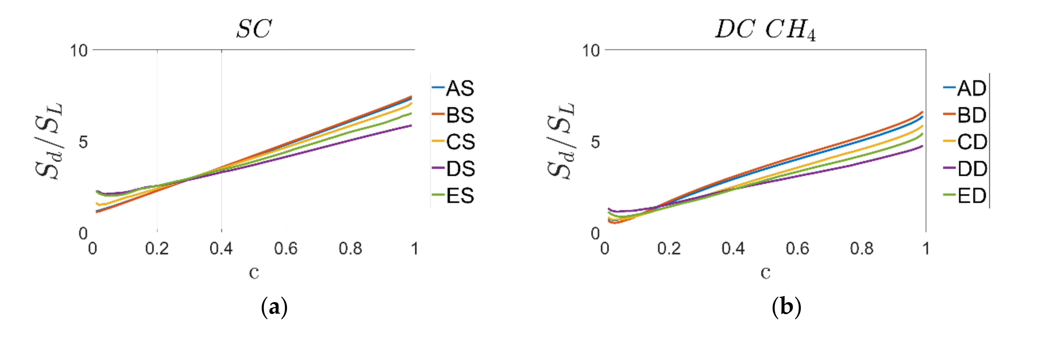
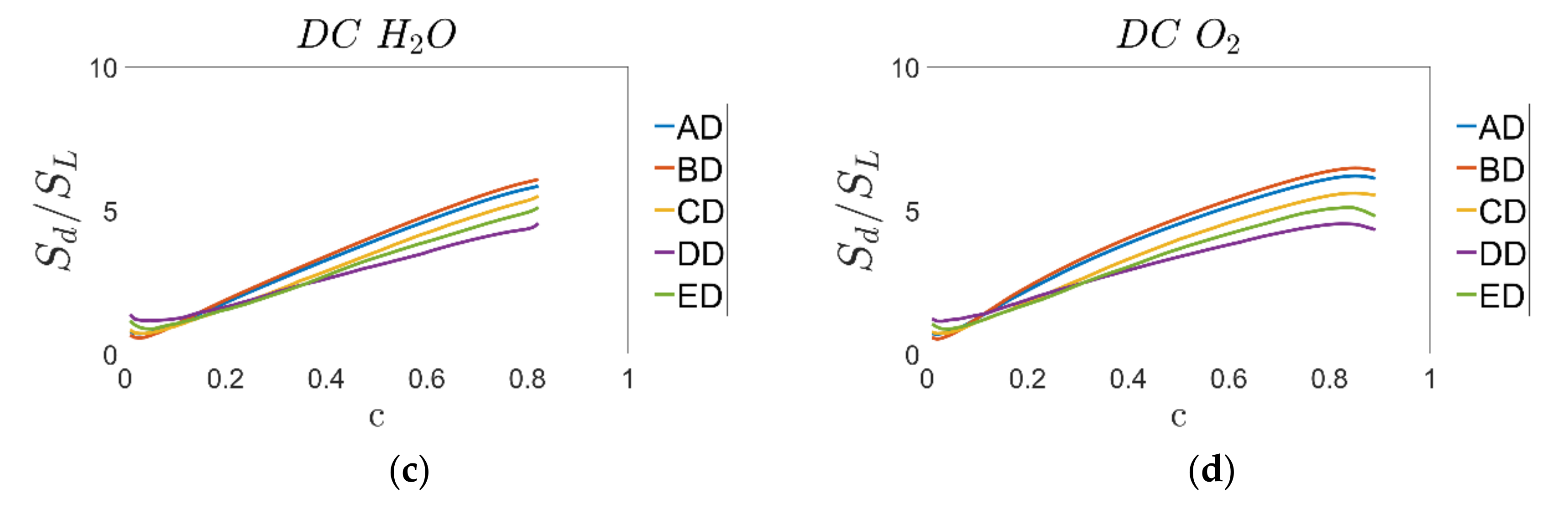
Mean variations of normalised displacement speed $S_d/S_L$ across the flame for all cases are shown in Figure 5 for SC and DC using three different definitions for reaction progress variable based on ${\mathrm{CH}}_4,{ \mathrm{H}}_2\mathrm{O}$ and ${\mathrm{O}}_2$ mass fractions. The variations between the different cases can be explained by stretch effects [23] and are consistent for all cases shown in Figure 5a–d. However, there are some non-negligible quantitative differences between the different definitions of $S_d$. The highest displacement speed values are obtained for the SC case and DC based on ${\mathrm{O}}_2$ mass fraction while the lowest values are achieved for ${\mathrm{CH}}_4$ mass fraction.

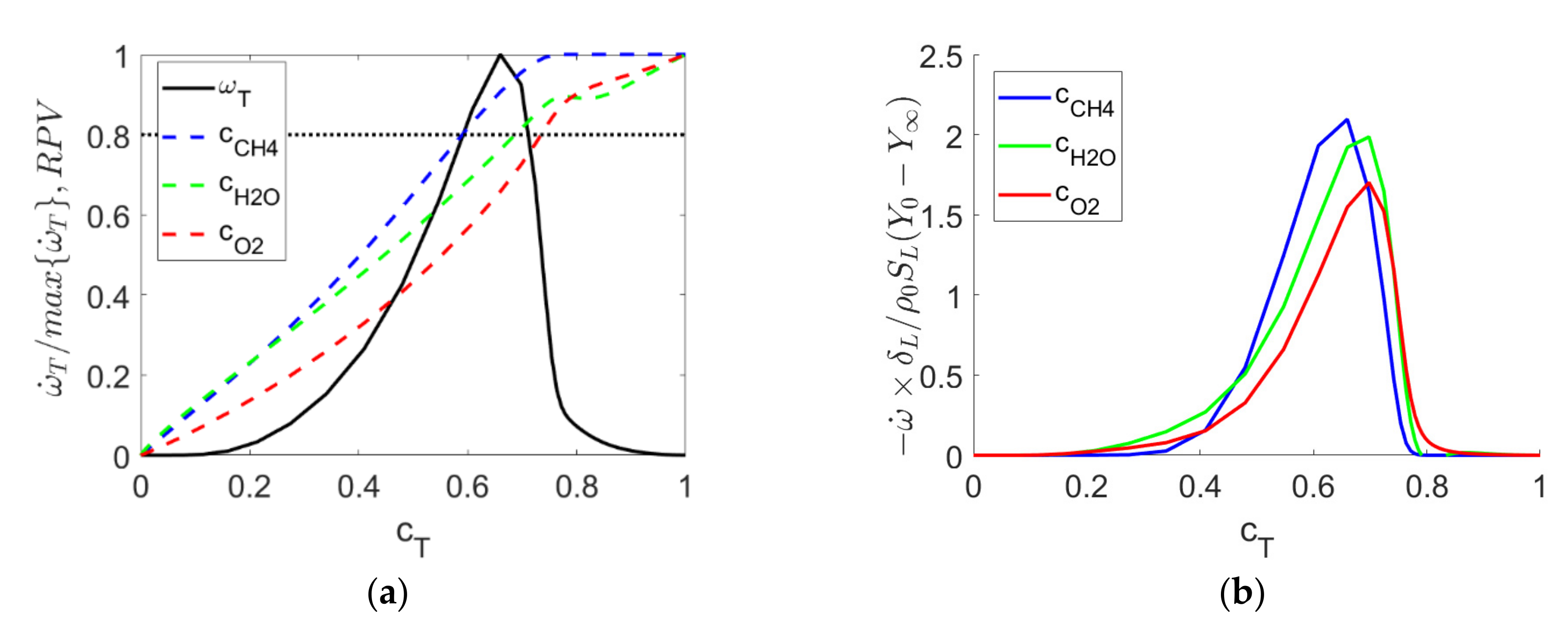
An advantage of the ${\mathrm{CH}}_4$ mass fraction-based reaction progress variable definition is that the displacement speed can be evaluated throughout the flame without any problems, while the ${\mathrm{H}}_2\mathrm{O}$ mass fraction-based definition becomes singular due to the non-monotonicity of ${\mathrm{H}}_2\mathrm{O}$-based reaction progress variable, as discussed earlier. Displacement speed defined by ${\mathrm{O}}_2$ mass fraction-based reaction progress variable becomes difficult to evaluate towards the burned gas side because $\left|\nabla c\right|$ assumes very small values before $c$ reaches a value of unity. It has to be admitted that there are quantitative differences between displacement speed statistics based on SC and DC simulations, however, they are of the same magnitude as the differences based on DC simulations using different definitions of reaction progress variable.

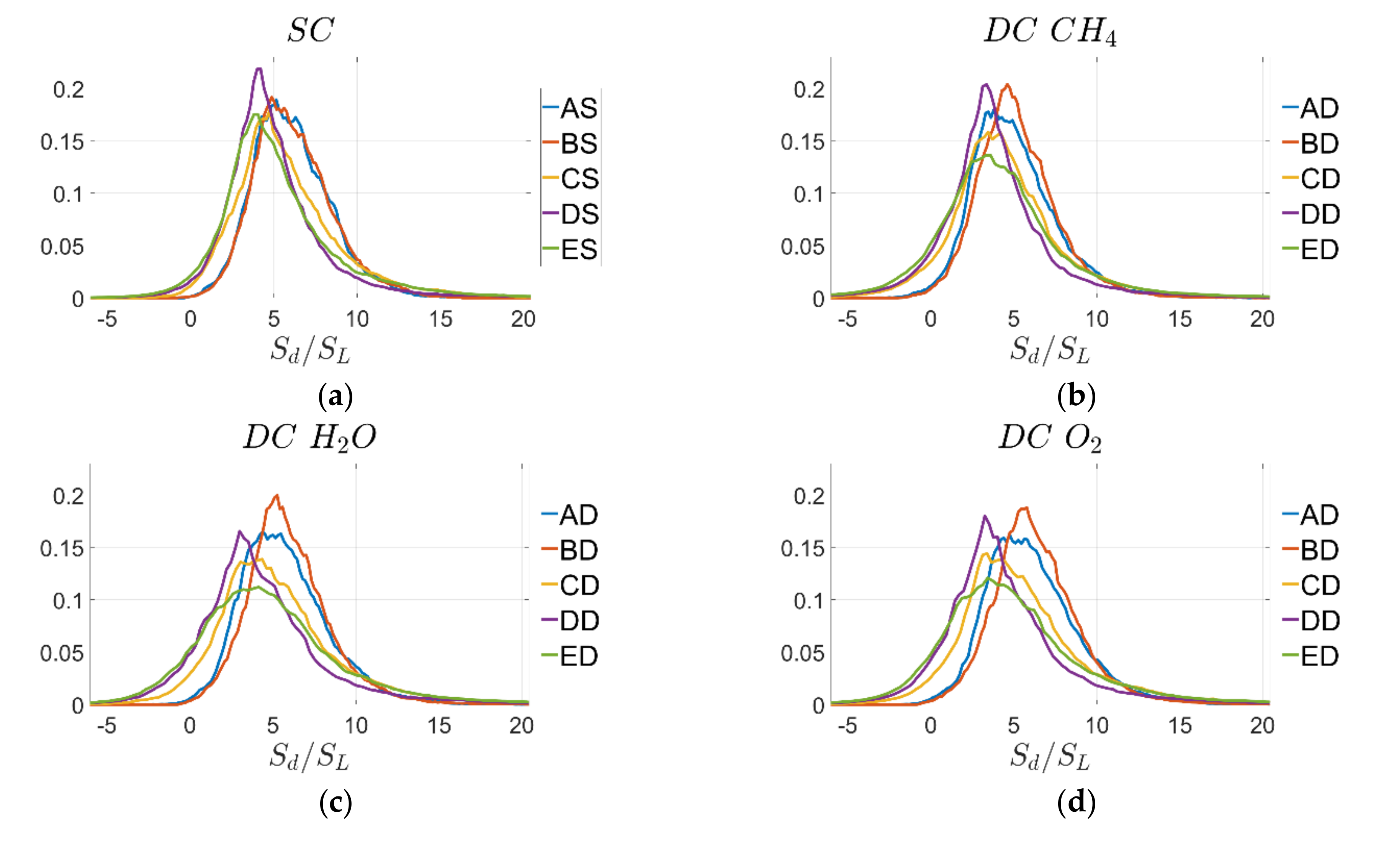
The behaviour observed from Figure 5 is consistent with the probability density functions (PDF) of normalised displacement speed $S_d/S_L$ on the $c=0.8$progress-variable isosurfaces, which are shown in Figure 6 for cases A–E and the quantitative evaluation of mean $E$ and standard deviation $\sigma$ of $S_d/S_L$ for $c=0.8$ are shown in

Table 6. Mean value $E$ and standard deviation δ of normalised displacement speed S_d/S_L for the $c=0.8$ isosurface for all cases.

	$\mathit{E}\left({\mathit{S}}_{\mathit{d}}\mathbf{/}{\mathit{S}}_{\mathit{L}}\right)$				$\mathit{\sigma }\left({\mathit{S}}_{\mathit{d}}\mathbf{/}{\mathit{S}}_{\mathit{L}}\right)$
Case	SC	$\mathbf{DC} \mathbf{C}{\mathbf{H}}_{\mathbf{4}}$	$\mathbf{DC} {\mathbf{H}}_{\mathbf{2}}\mathbf{O}$	DC ${\mathbf{O}}_{\mathbf{2}}$	SC	$\mathbf{DC} \mathbf{C}{\mathbf{H}}_{\mathbf{4}}$	$\mathbf{DC} {\mathbf{H}}_{\mathbf{2}}\mathbf{O}$	DC ${\mathbf{O}}_{\mathbf{2}}$
A	6.08	5.03	5.75	6.10	2.33	2.58	2.71	2.80
B	6.15	5.24	5.98	6.37	2.35	2.47	2.56	2.64
C	5.83	4.56	5.34	5.51	3.40	3.59	3.95	4.05
D	5.04	3.81	4.35	4.51	3.42	3.70	4.26	4.31
E	5.49	4.20	4.93	5.05	4.76	4.22	4.92	4.98

. Table 6 indicates that the values of $\sigma \left(S_d/S_L\right)$ can be split into three groups, cases A, B, cases C, D and case E, and this behaviour is consistent for all cases and in particular when comparing SC and DC.

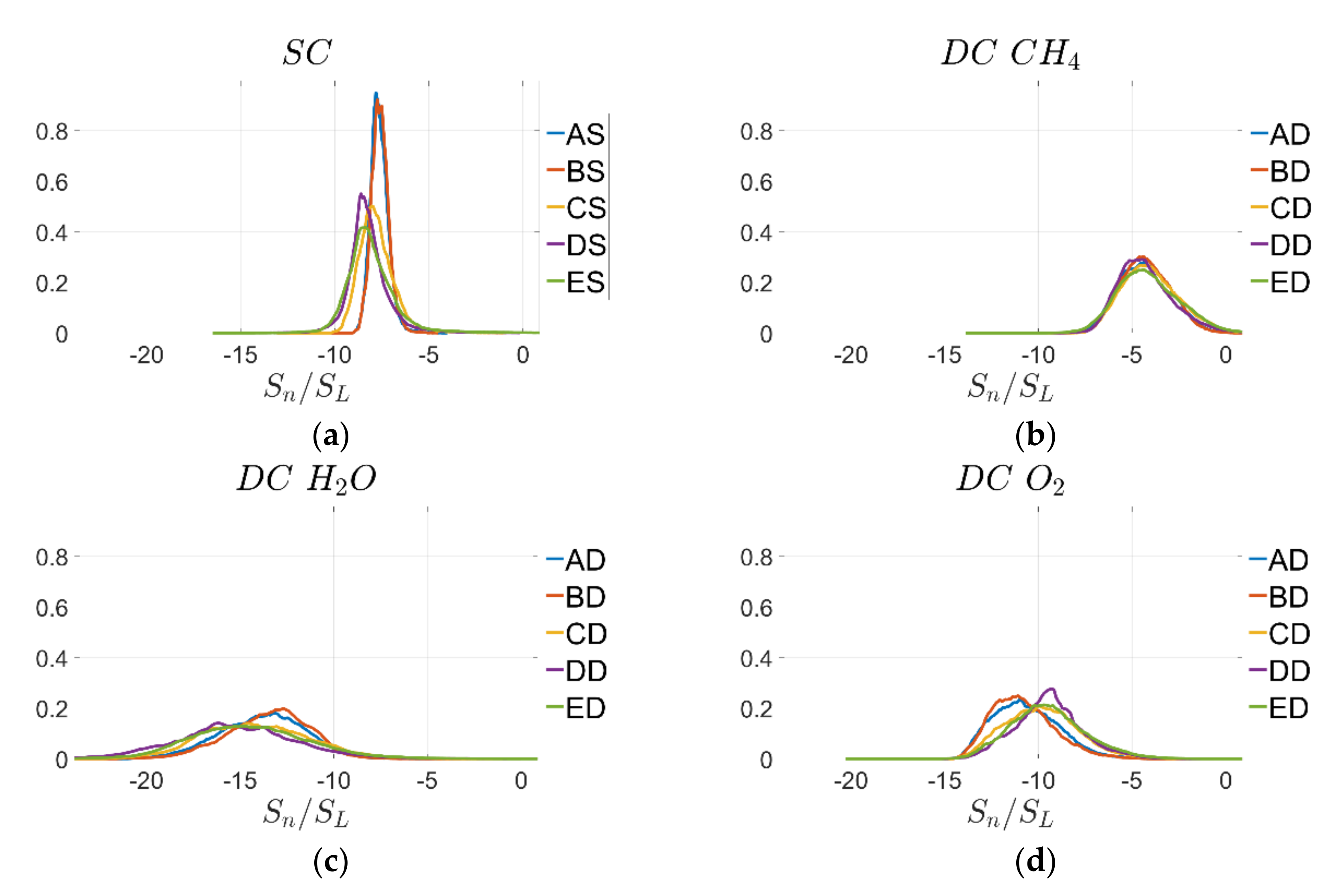
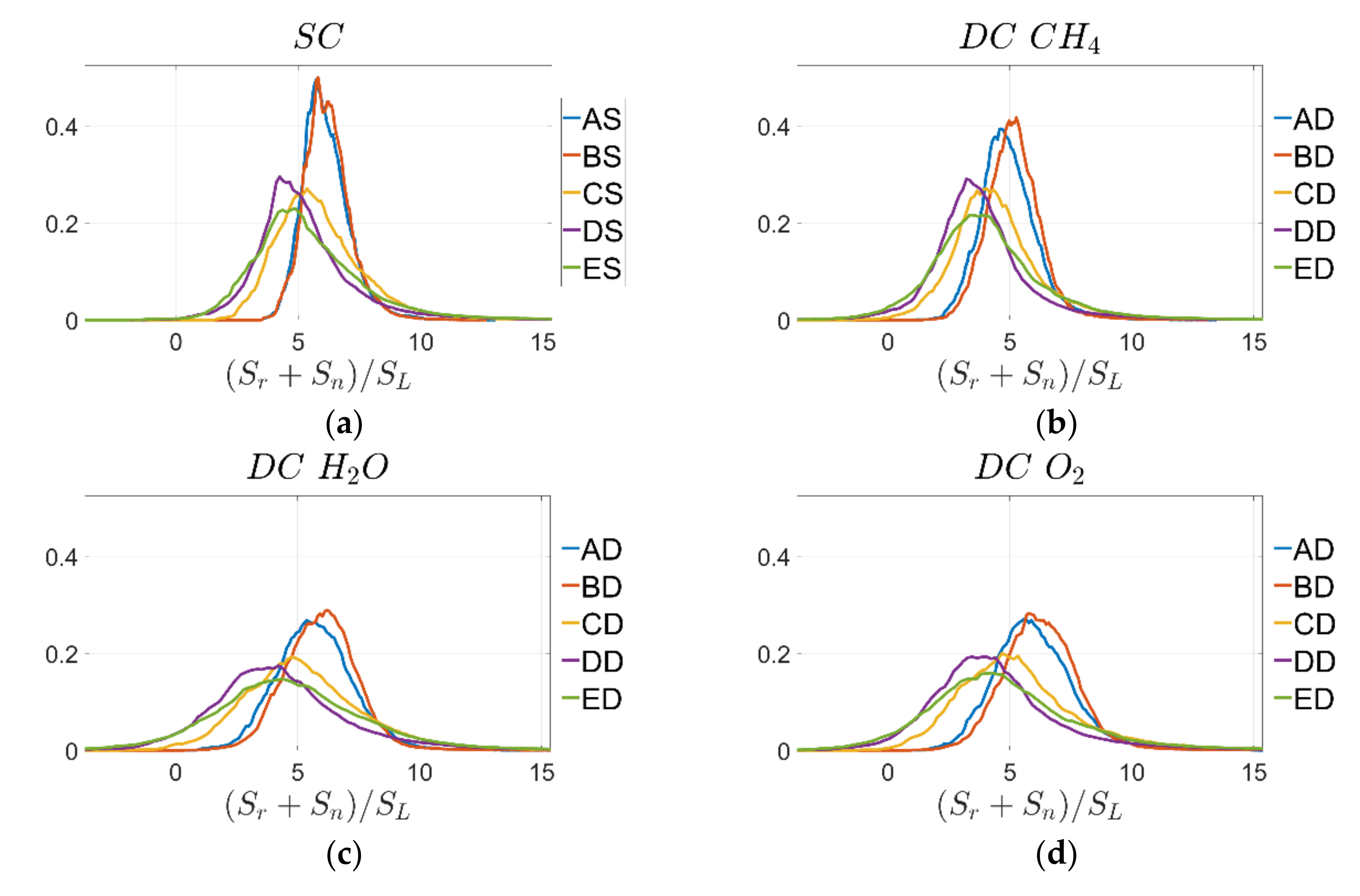
Similar trends can be observed for the PDF of normalised combined reaction and normal diffusion components of displacement speed $\left(S_r+S_n\right)/S_L$ shown for the $c=0.8$isosurface in Figure 7. It is noted that the DC PDFs for reaction progress variable based on ${\mathrm{H}}_2\mathrm{O}$ and ${\mathrm{O}}_2$ mass fractions tend to be wider than those for SC and DC based on ${\mathrm{CH}}_4$. This behaviour will be analysed in more detail by looking next at the individual contributions $S_r,S_n,S_t$, and the corresponding PDFs for $c=0.8$ are shown in Figure 7, Figure 8 and Figure 9, while the corresponding mean values and standard deviations for $S_r$ and $S_n$ are shown in

Table 7. Mean value $E$ and standard deviation $\sigma$ of normalised displacement speed $S_n/S_L$ for the $c=0.8$ isosurface value for all cases.

	$\mathit{E}\left({\mathit{S}}_{\mathit{n}}\mathbf{/}{\mathit{S}}_{\mathit{L}}\right)$				$\mathit{\sigma }\left({\mathit{S}}_{\mathit{n}}\mathbf{/}{\mathit{S}}_{\mathit{L}}\right)$
Case	SC	$\mathbf{DC} \mathbf{C}{\mathbf{H}}_{\mathbf{4}}$	$\mathbf{DC} {\mathbf{H}}_{\mathbf{2}}\mathbf{O}$	DC ${\mathbf{O}}_{\mathbf{2}}$	SC	$\mathbf{DC} \mathbf{C}{\mathbf{H}}_{\mathbf{4}}$	$\mathbf{DC} {\mathbf{H}}_{\mathbf{2}}\mathbf{O}$	DC ${\mathbf{O}}_{\mathbf{2}}$
A	−7.62	−4.32	−13.77	−10.66	1.40	2.16	2.91	1.86
B	−7.59	−4.27	−13.49	−10.83	1.39	2.13	2.86	1.77
C	−7.77	−4.00	−14.14	−9.84	1.66	2.21	3.38	2.04
D	−8.22	−4.27	−15.17	−9.45	1.93	2.18	3.70	1.95
E	−8.02	−4.09	−14.46	−9.48	2.21	2.31	3.60	2.14

and

Table 8. Mean value $E$ and standard deviation $\sigma$ of normalised displacement speed $S_r/S_L$ for the $c=0.8$ isosurface value for all cases.

	$\mathit{E}\left({\mathit{S}}_{\mathit{r}}\mathbf{/}{\mathit{S}}_{\mathit{L}}\right)$				$\mathit{\sigma }\left({\mathit{S}}_{\mathit{r}}\mathbf{/}{\mathit{S}}_{\mathit{L}}\right)$
Case	SC	$\mathbf{DC} \mathbf{C}{\mathbf{H}}_{\mathbf{4}}$	$\mathbf{DC} {\mathbf{H}}_{\mathbf{2}}\mathbf{O}$	DC ${\mathbf{O}}_{\mathbf{2}}$	SC	$\mathbf{DC} \mathbf{C}{\mathbf{H}}_{\mathbf{4}}$	$\mathbf{DC} {\mathbf{H}}_{\mathbf{2}}\mathbf{O}$	DC ${\mathbf{O}}_{\mathbf{2}}$
A	13.75	9.27	19.50	16.66	1.51	2.53	2.51	2.80
B	13.77	9.46	19.45	17.11	1.51	2.49	2.53	2.65
C	13.65	8.53	19.51	15.29	1.73	2.75	2.46	3.91
D	13.48	8.10	19.60	13.97	2.04	2.62	2.90	4.10
E	13.64	8.21	19.31	14.40	2.58	2.84	2.65	4.58

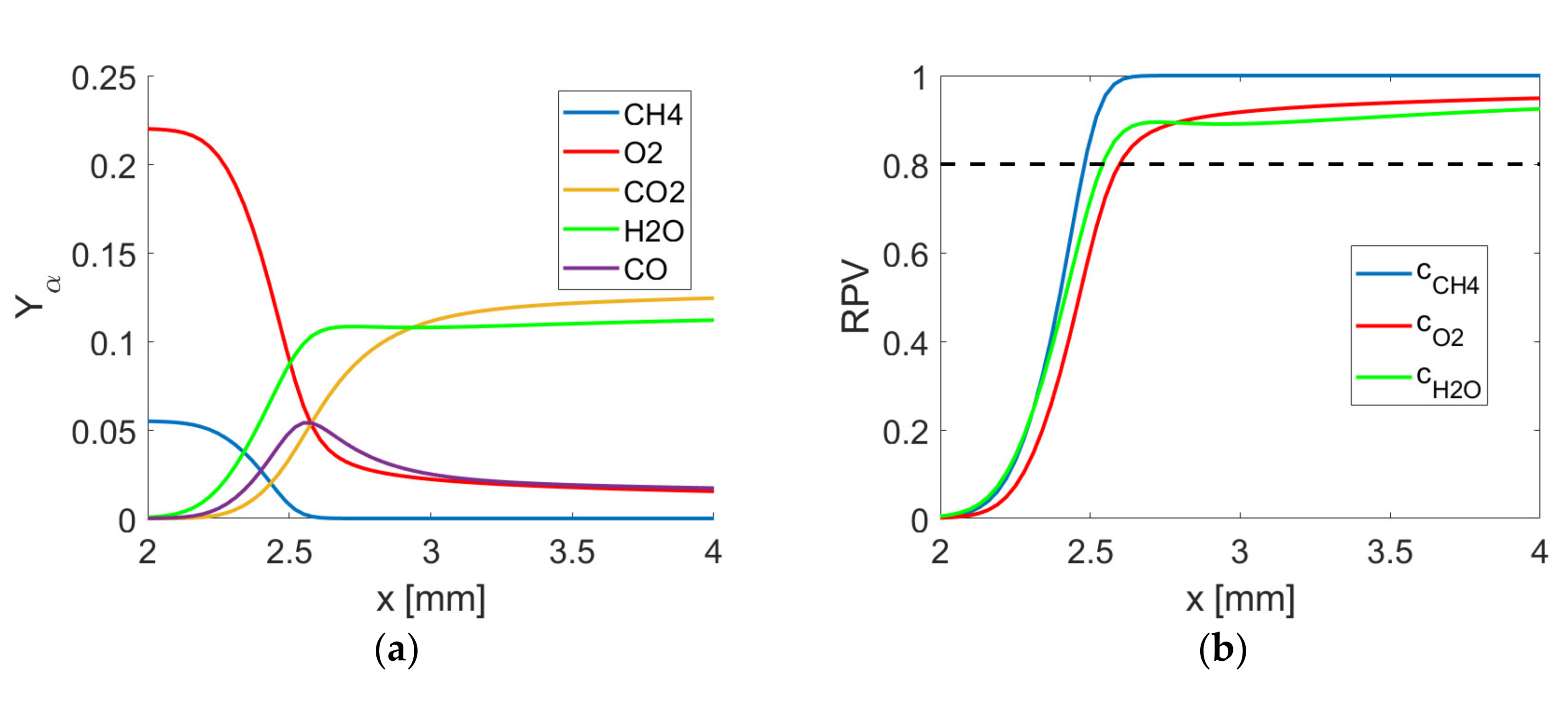
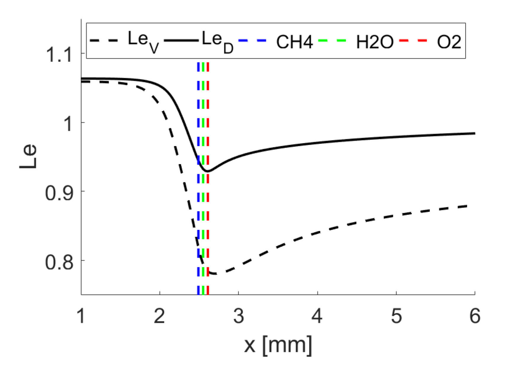
. The mean value of $S_t$ is close to zero for a statistically planar flame and therefore these numbers are not shown in the form of a table. Figure 8 and Table 7 indicate that the mean values of $S_n/S_L$ are close to each other for all cases but there are differences based on the different definitions of reaction progress variable. This indicates that the differences in the PDFs of normal diffusion components are driven by the significant differences in the laminar profiles of reaction progress variable across the flame brush when using different species mass fractions for its definition as shown in Figure 2b and Figure 3a. It is also noted that the width of the PDFs of $S_n/S_L$ tends to be larger for the DC cases compared to the SC simulations. A possible explanation is that $\rho D_c$ can be taken as a constant for SC simulations while $\rho D_c$ is temperature-dependent in the DC cases, and hence is likely to introduce additional variations for the DC setup due to the decoupling of reaction progress variable and temperature (see Figure 3). Furthermore, as noted earlier, the SC simulations have higher viscosity and hence slightly smaller turbulence intensity at the time when statistics are taken.

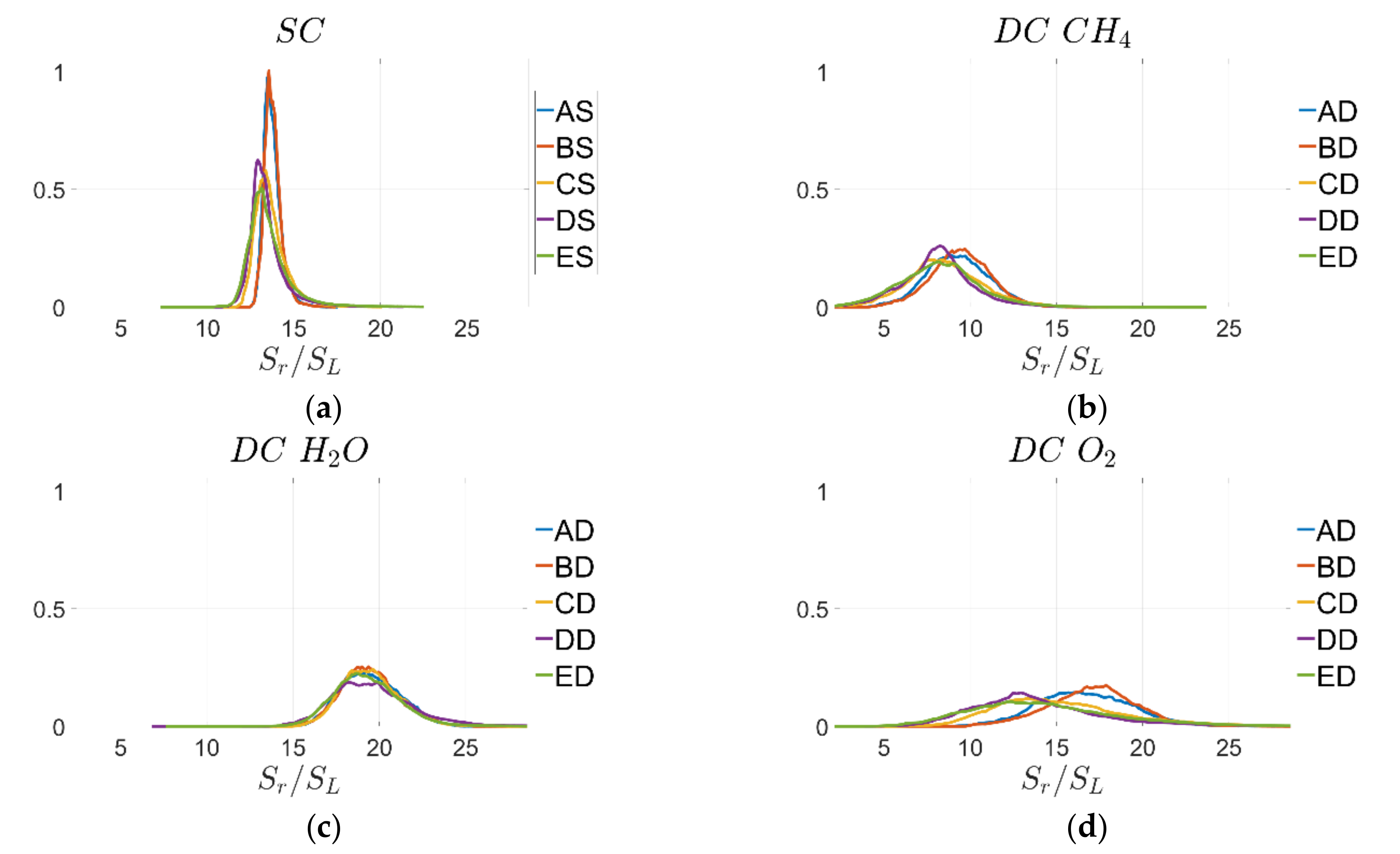
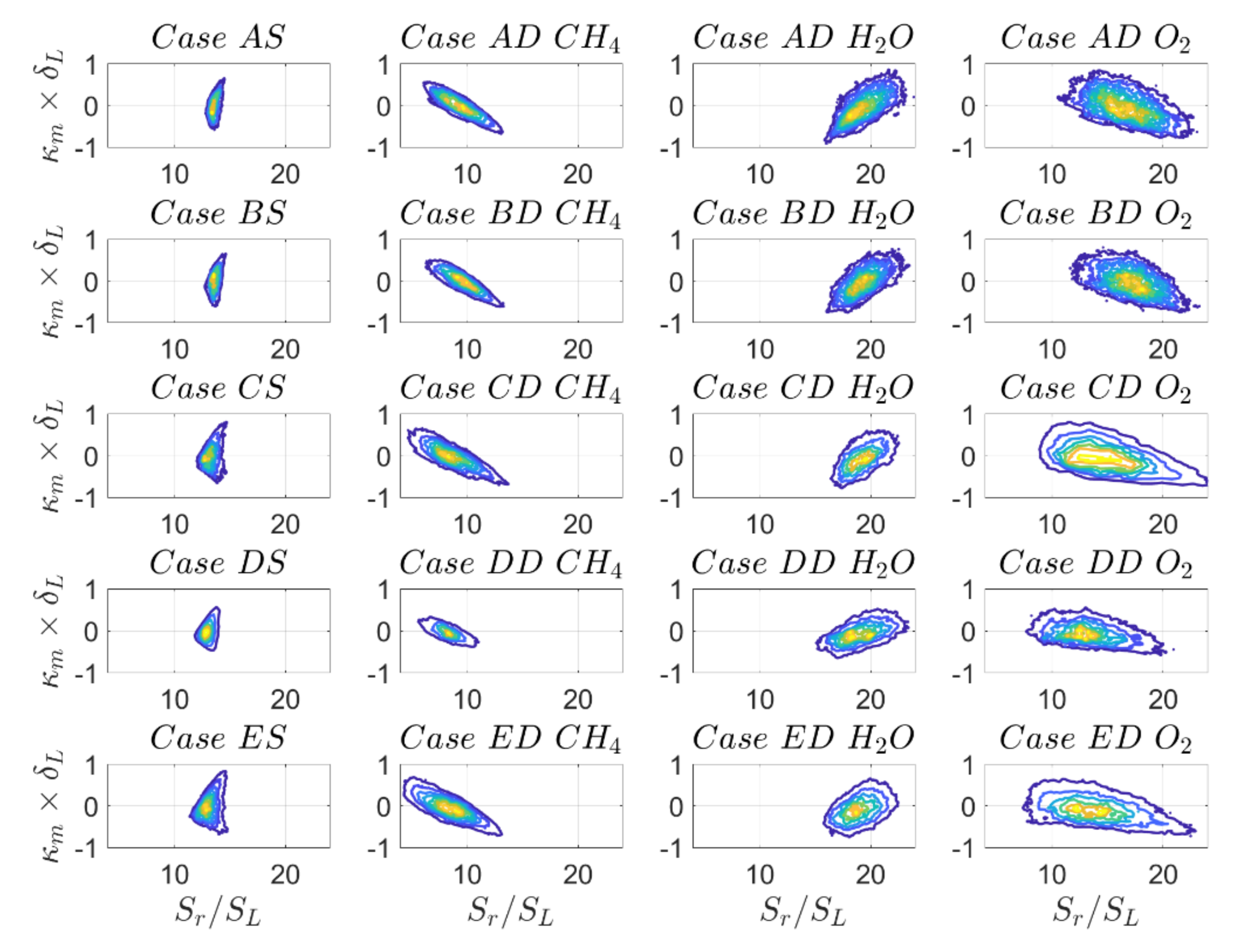
The PDFs of the normalised reaction component of displacement speed $S_r/S_L$ for the $c=0.8$ isosurface are shown in Figure 9 and the first and second moments for the $c=0.8$ reaction progress variable value are given in Table 8. The mass fractions of ${\mathrm{CH}}_4,{\mathrm{H}}_2\mathrm{O}$ and ${\mathrm{O}}_2$ have different values at the location of maximum heat release. Thus, it is not surprising that they show moderate differences in mean values depending on the definition of reaction progress variable. For SC, the mean values of $S_r/S_L$ are nearly identical for all cases considered here, while for the DC simulations there is more variability (in particular for reaction progress variable based on ${\mathrm{CH}}_4$ and ${\mathrm{O}}_2$ mass fractions) depending on the initial turbulence intensity. This can be explained in the following manner. For simple chemistry, low Mach number and unity Lewis number simulations, reaction progress variable and non-dimensional temperature are identical and consequently the reaction rate $\dot{{\omega }_c}$is a unique function of $c$. In contrast, for the DC case, the reaction rate of an individual species depends not only on temperature but also on the reaction progress of several other species. Furthermore, the standard enthalpy of formation of a pure element is zero which shows that $\dot{{\omega }_c}$(and equally ${\dot{\omega }}_{\alpha }$) and ${\dot{\omega }}_T$ are not always directly related. Hence, a change of reaction progress variable in the DC case is less directly interlinked with a change in temperature. In all cases (including DC), the turbulent motion of the fluid causes variations of the surface density function $\left|\nabla c\right|$ (which scales with the inverse flame thickness) in such a manner that the variance of $S_r/S_L$ increases from case A to case E.

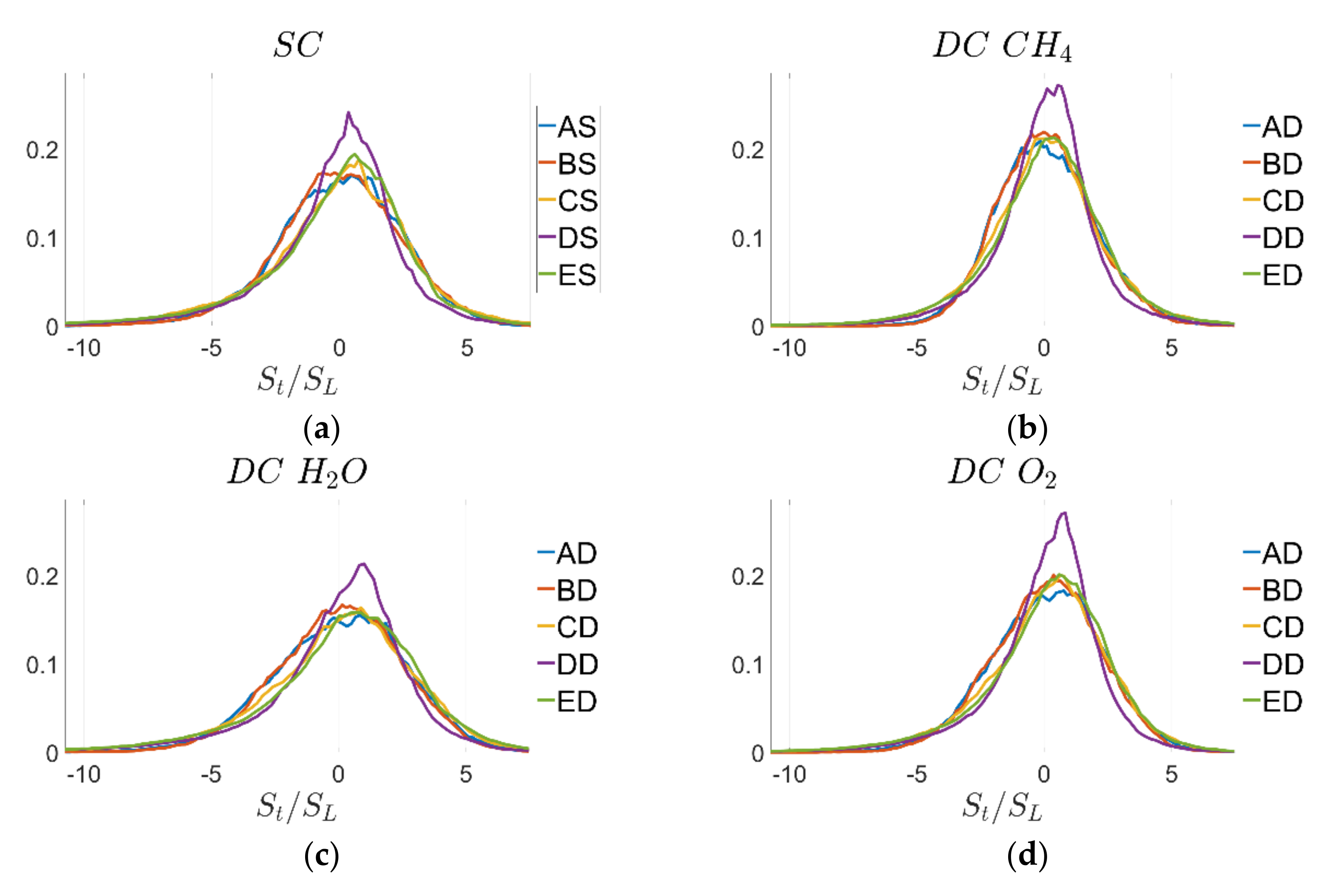
Despite the remarkable differences of the PDFs of $S_r$ and $S_n$ for the different definitions of reaction progress variable, the reaction–diffusion balance in the expression $\left(S_r+S_n\right)$ remains qualitatively much more similar compared to the individual contributions as discussed before, because a more positive value of $S_r$ is balanced by a more negative value of $S_n$ and vice versa. Finally, the PDFs of normalised tangential diffusion component of displacement speed $S_t/S_L$ for the $c=0.8$ isosurface are shown in Figure 10. Due to the statistically planar nature of the flames considered here, their mean value is close to zero in all cases and the standard deviation has the same order of magnitude for all definitions of reaction progress variable but tends to increase with increasing turbulence intensity.

The statistics of $S_d,\left(S_r+S_n\right), S_t$ remain qualitatively, and to a large extent quantitatively similar for SC and DC simulations and also for different definitions of reaction progress variable. However, there are marked qualitative differences for individual contributions of displacement speed $S_r$ and $S_n$. To explain this behaviour, it is important to understand their interrelation with curvature and strain rate as well as the influence of the definition of reaction progress variable, which will be discussed in the next subsection.

3.2. Curvature and Tangential Strain Rate Effects on Local Displacement Speed and Its Components

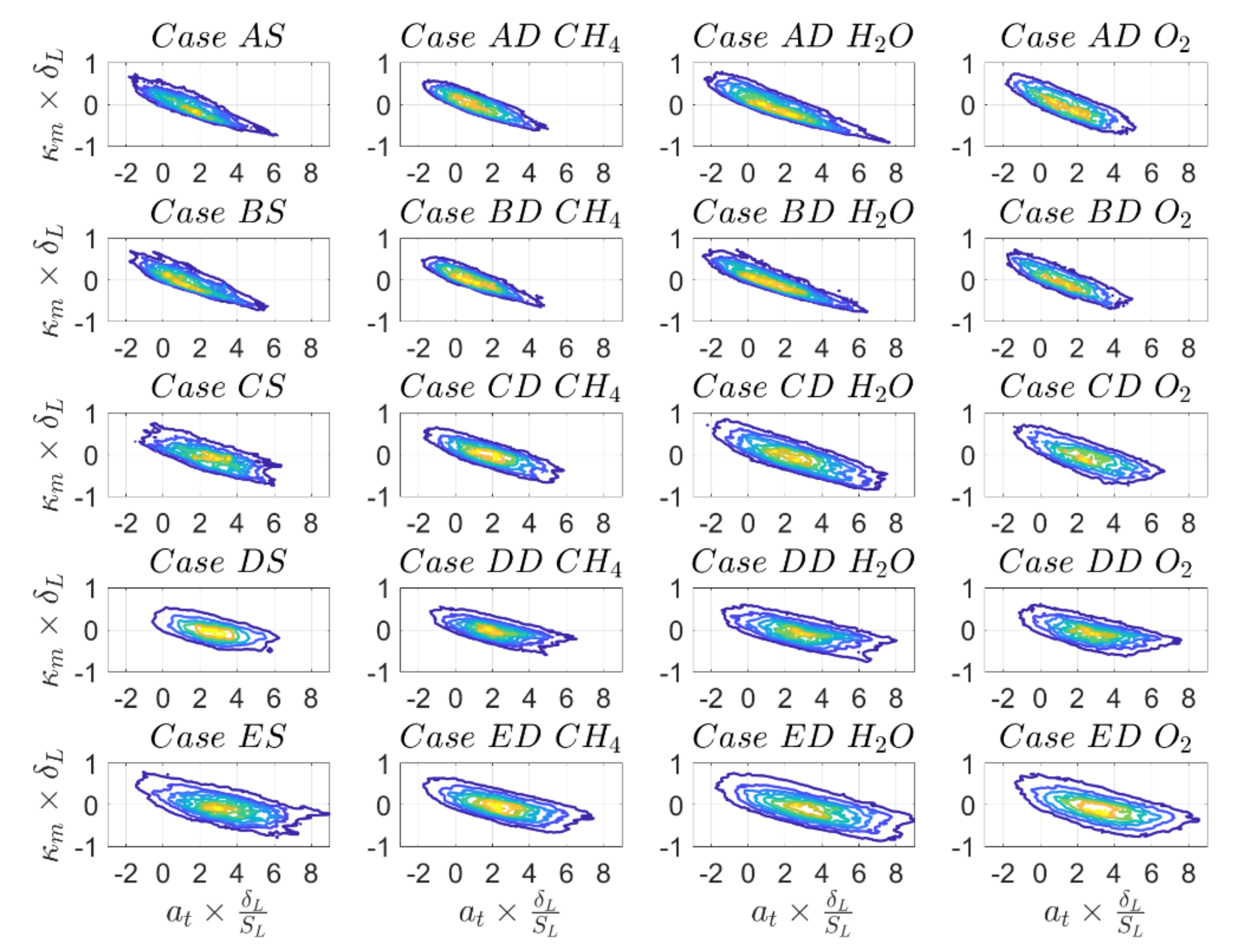
Theoretical studies suggest that flame stretch is the controlling parameter of the flame structure in the limit of weak turbulence and weak flame wrinkling (for an overview see [26,47]). Flame stretch rate is, in turn, a function of flame curvature ${\kappa }_m$ and tangential strain rate $a_T=\left({\delta }_{ij}-N_i{N}_j\right)\partial u_i/\partial x_j$. The PDFs of $a_T$ and ${\kappa }_m$ have been discussed in part 1 of this paper and do not provide additional insight here. Their joint PDFs are shown in Figure 11 and the correlation coefficients between $a_T$ and ${\kappa }_m$ are reported in

Table 9. Correlation coefficients between tangential strain rate and curvature for the $c=0.8$ isosurface value for all cases.

	$\mathit{c}\mathit{o}\mathit{r}\mathit{r}\left({\mathit{a}}_{\mathit{T}},{\mathit{\kappa }}_{\mathit{m}}\right)$
Case	SC	$\mathbf{DC} \mathbf{C}{\mathbf{H}}_{\mathbf{4}}$	$\mathbf{DC} {\mathbf{H}}_{\mathbf{2}}\mathbf{O}$	DC ${\mathbf{O}}_{\mathbf{2}}$ Isosurface Value for All Cases
A	−0.86	−0.88	−0.89	−0.84
B	−0.85	−0.88	−0.89	−0.83
C	−0.79	−0.82	−0.81	−0.75
D	−0.62	−0.66	−0.66	−0.59
E	−0.65	−0.70	−0.70	−0.62

for $c=0.8$.

It can be seen from Figure 11 that there is a negative correlation between $a_T$ and ${\kappa }_m$ in all cases which is the strongest for cases A and B and weakest for cases D and E. The correlation strength is weakly dependent on the definition of reaction progress variable. These results are in very good agreement with an earlier analysis reported in [49]. As $a_T$ and ${\kappa }_m$ are not independent parameters, the dependence of $S_d$ and its components with $a_T$ can be deduced from the interrelation of $S_d$ and its components with ${\kappa }_m$ and vice versa. Therefore, the following discussion is limited to correlations of displacement speed and its components with mean curvature.

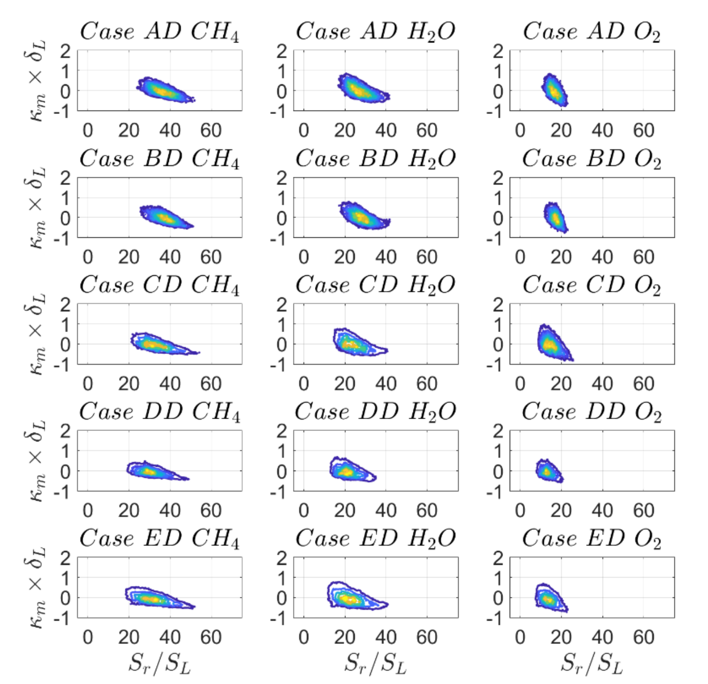
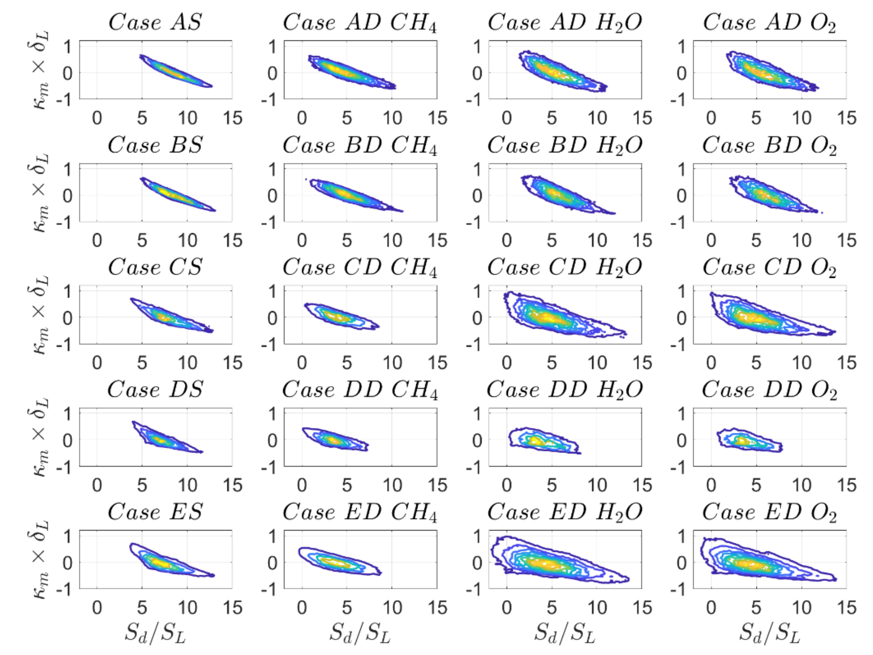
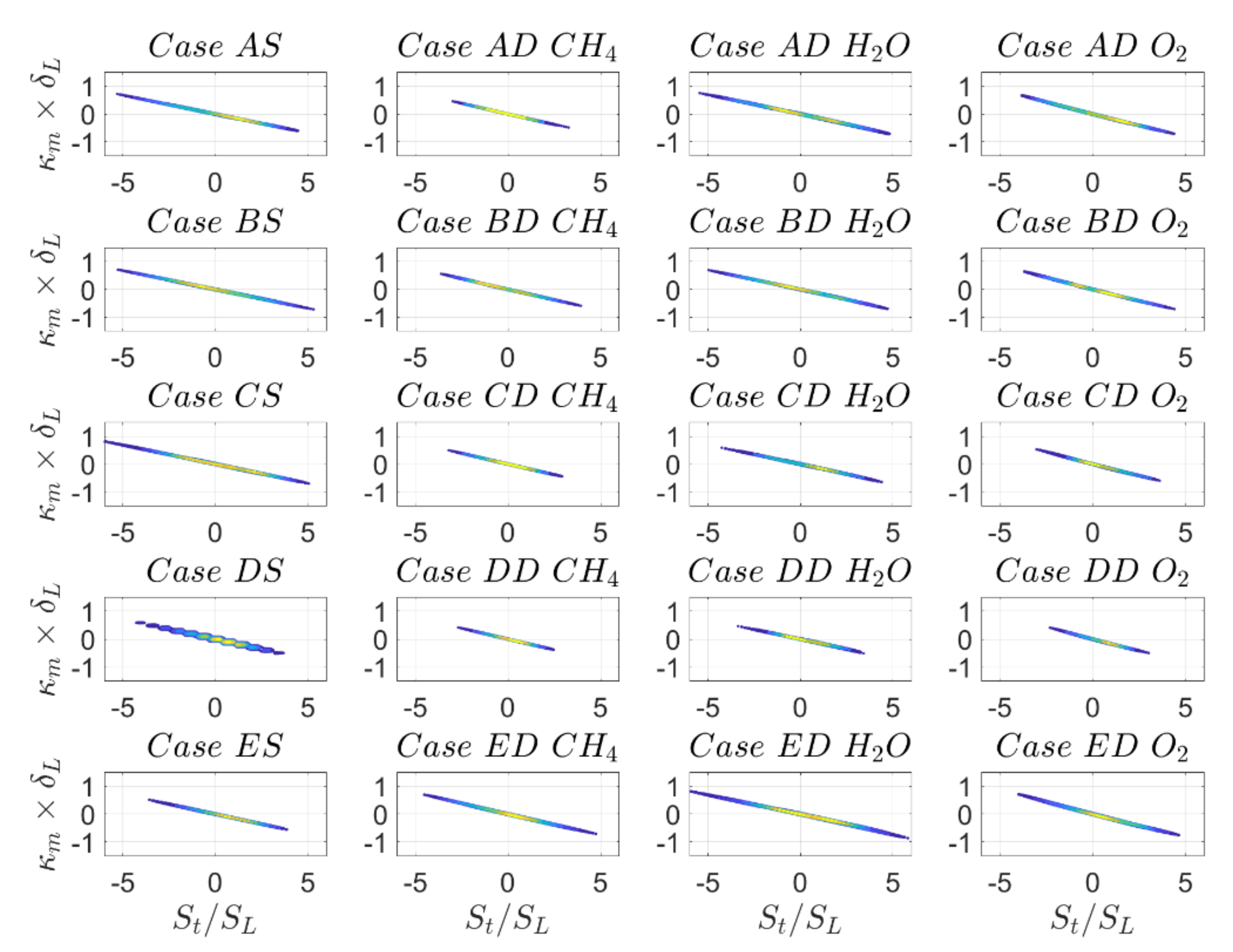
The joint PDFs of $S_d$ and $\left(S_r+S_n\right)$ with ${\kappa }_m$ are shown in Figure 12 and Figure 13, respectively for the $c=0.8$ isosurface and the corresponding correlation coefficients are reported in

Table 10. Correlation coefficients between $S_d$ and $\left(S_r+S_n\right)$ with ${\kappa }_m$ for the $c=0.8$ isosurface value for all cases.

	$\mathit{c}\mathit{o}\mathit{r}\mathit{r}\left({\mathit{S}}_{\mathit{d}}\mathbf{,}{\mathit{\kappa }}_{\mathit{m}}\right)$				$\mathit{c}\mathit{o}\mathit{r}\mathit{r}\left({\mathit{S}}_{\mathit{r}}\mathbf{+}{\mathit{S}}_{\mathit{n}}\mathbf{,}{\mathit{\kappa }}_{\mathit{m}}\right)$
Case	SC	$\mathbf{DC} \mathbf{C}{\mathbf{H}}_{\mathbf{4}}$	$\mathbf{DC} {\mathbf{H}}_{\mathbf{2}}\mathbf{O}$	DC ${\mathbf{O}}_{\mathbf{2}}$	SC	$\mathbf{DC} \mathbf{C}{\mathbf{H}}_{\mathbf{4}}$	$\mathbf{DC} {\mathbf{H}}_{\mathbf{2}}\mathbf{O}$	DC ${\mathbf{O}}_{\mathbf{2}}$
A	−0.92	−0.89	−0.83	−0.79	0.30	−0.29	0.25	−0.01
B	−0.92	−0.89	−0.83	−0.80	0.27	−0.29	0.24	−0.01
C	−0.83	−0.85	−0.74	−0.72	0.02	−0.38	0.09	−0.14
D	−0.73	−0.82	−0.66	−0.65	0.14	−0.38	0.09	−0.13
E	−0.65	−0.83	−0.70	−0.67	0.01	−0.40	0.00	−0.18

for $c=0.8$. It can be seen from Figure 12 that displacement speed is negatively correlated with mean curvature. While the correlation coefficients are close to $-1.0$ for cases A and B, the correlation becomes non-linear for increasing turbulence intensity, as can be discerned from the considerably smaller values of $corr\left(S_d,{\kappa }_m\right)$ in comparison to −1.0. Table 10 also shows that the strength of linearity or non-linearity depends to some extent on the physio-chemical model and also on the definition of reaction progress variable in the case of DC. Tangential diffusion component of displacement speed $S_t$ is deterministically negatively correlated with curvature (see Equation (8)) with $corr\left(S_t,{\kappa }_m\right)<-0.99$ in all cases, and for all definitions of reaction progress variable, as illustrated in Figure 14. This shows that the non-linear curvature dependence of $S_d$ originates from the non-linear curvature dependence of $(S_r+S_n)$. For $c=0.8$, the correlation strength between $\left(S_r+S_n\right)$ is weak in all cases. Figure 13 and Table 10 show that there is a weak positive correlation in the case of both SC and DC simulations based on the reaction progress variable defined in terms of ${\mathrm{H}}_2\mathrm{O}$ while the correlation turns out to be mildly negative for DC and reaction progress variable based on ${\mathrm{CH}}_4$ and ${\mathrm{O}}_2$ mass fractions. Again, for SC, the behaviour is in good agreement with the DC results and detailed explanations are also provided for the change of correlation strength with the value of reaction progress variable [49], while the present analysis focuses on the differences between SC and DC and also on the differences resulting from different definitions of reaction progress variable.

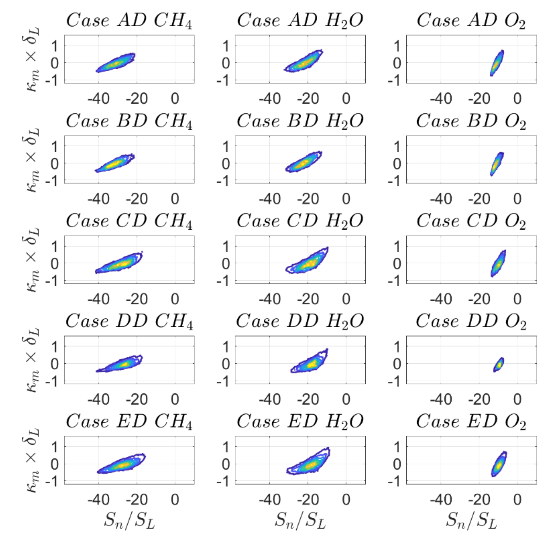
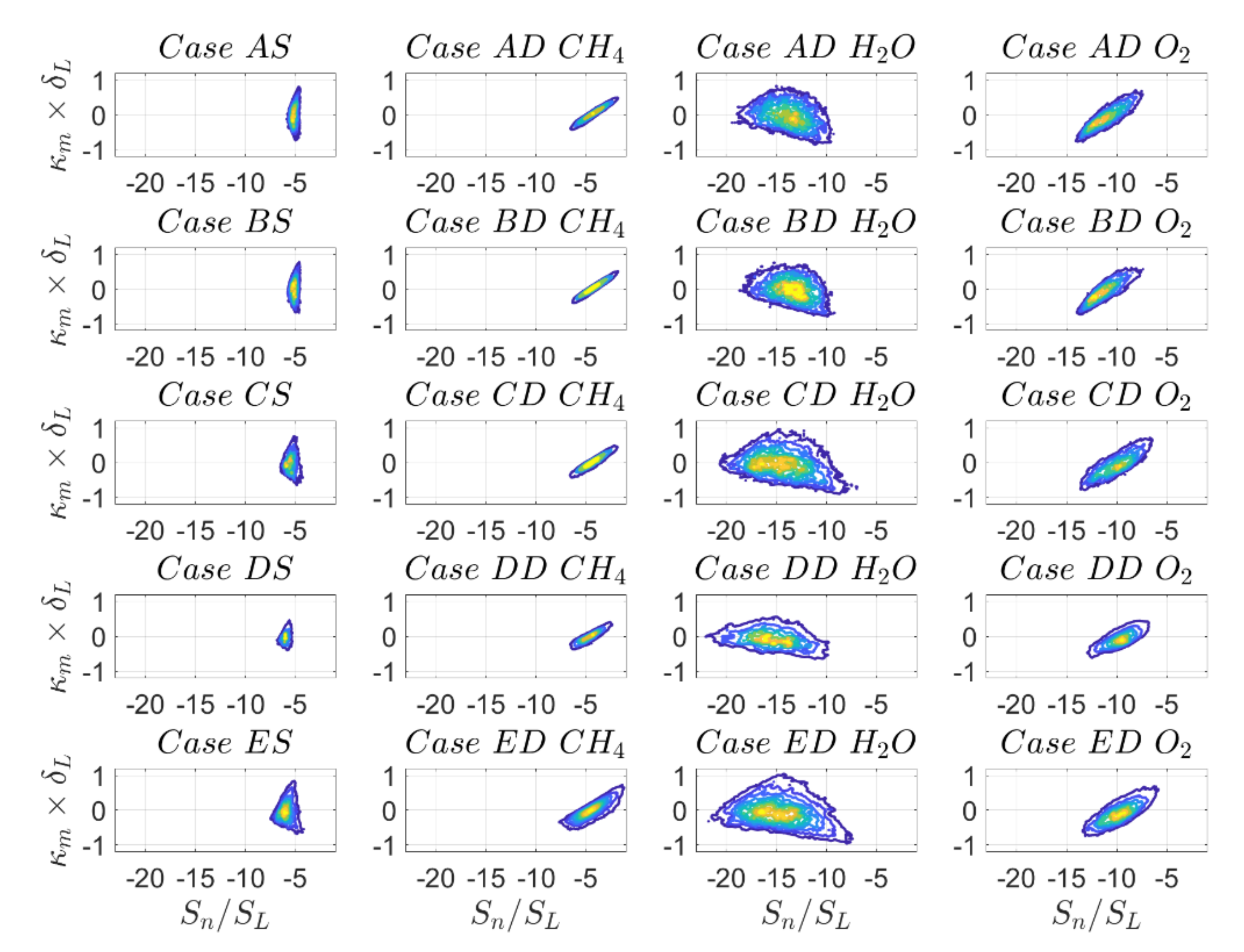
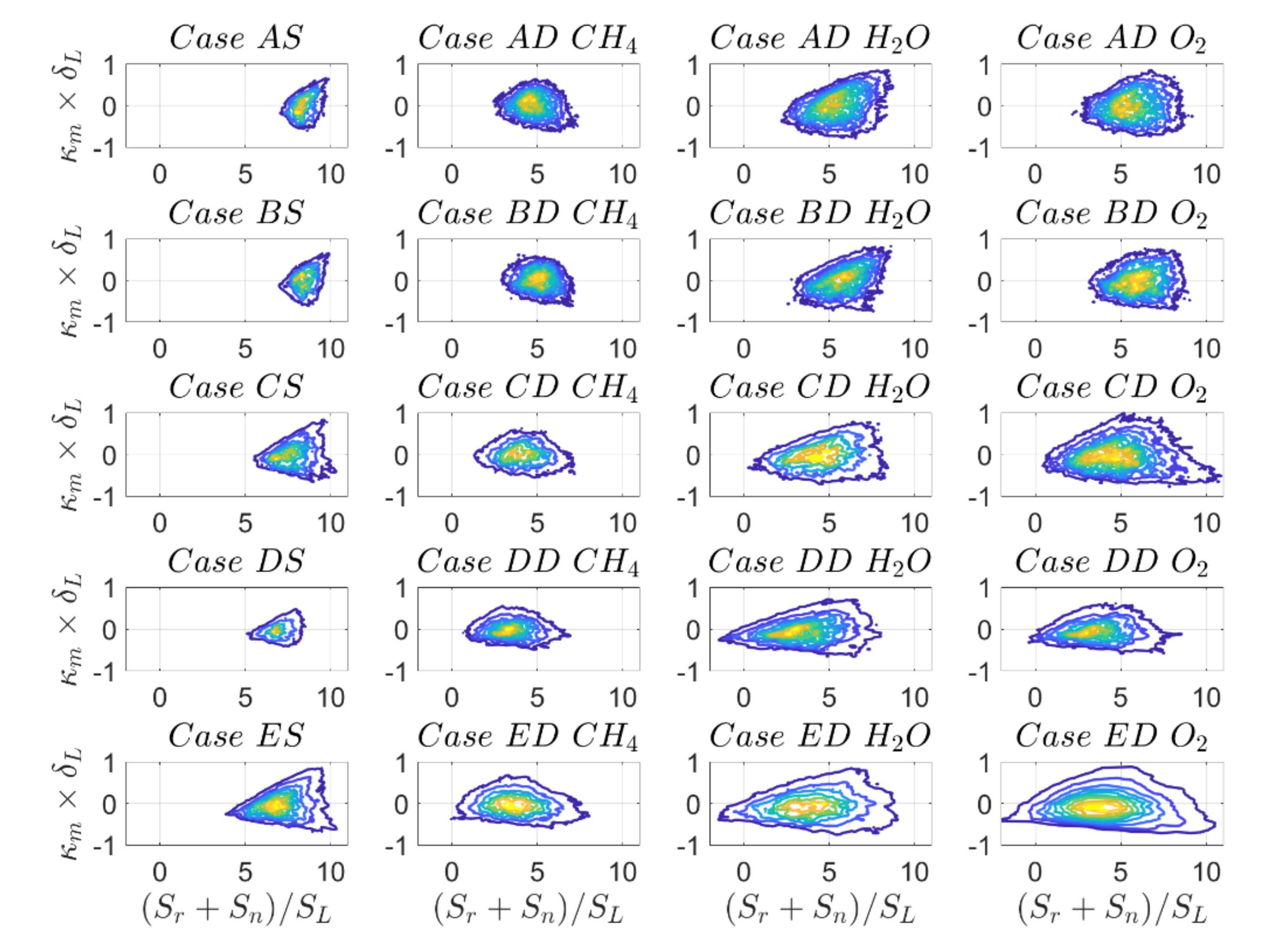
So far, results have revealed a reasonable qualitative agreement of displacement speed statistics with some quantitative variations when comparing DC with SC, which are of the same order of magnitude, as compared to different definitions of reaction progress variable in the case of DC. As illustrated in Figure 15 and Figure 16, this behaviour changes drastically when looking at the individual contributions of displacement speed $S_r$ and $S_n$ with mean curvature. For example, there is a weak positive correlation $corr\left(S_r,{\kappa }_m\right)$ in the case of SC and DC based on ${\mathrm{H}}_2\mathrm{O}$ mass fraction, whereas the correlation is clearly negative in the case of DC with reaction progress variable based on ${\mathrm{CH}}_4$ and ${\mathrm{O}}_2$ mass fractions for the reaction progress variable isosurface $c=0.8$. In other words, there is a qualitative change in $corr\left(S_r,{\kappa }_m\right)$ with the variation of the definition of reaction progress variable, which warrants further explanation. Similar qualitative differences can be seen from the $S_n-{\kappa }_m$ joint PDFs shown in Figure 16. The values of $corr\left(S_r,{\kappa }_m\right)$ and $corr\left(S_n,{\kappa }_m\right)$are reported in

Table 11. Correlation coefficients between $S_r$ and $S_n$ with ${\kappa }_m$ for the $c=0.8$ isosurface value for all cases.

	$\mathit{c}\mathit{o}\mathit{r}\mathit{r}\left({\mathit{S}}_{\mathit{r}}\mathbf{,}{\mathit{\kappa }}_{\mathit{m}}\right)$				$\mathit{c}\mathit{o}\mathit{r}\mathit{r}\left({\mathit{S}}_{\mathit{n}}\mathbf{,}{\mathit{\kappa }}_{\mathit{m}}\right)$
Case	SC	$\mathbf{DC} \mathbf{C}{\mathbf{H}}_{\mathbf{4}}$	$\mathbf{DC} {\mathbf{H}}_{\mathbf{2}}\mathbf{O}$	DC ${\mathbf{O}}_{\mathbf{2}}$	SC	$\mathbf{DC} \mathbf{C}{\mathbf{H}}_{\mathbf{4}}$	$\mathbf{DC} {\mathbf{H}}_{\mathbf{2}}\mathbf{O}$	DC ${\mathbf{O}}_{\mathbf{2}}$
A	0.16	−0.61	0.46	−0.54	0.04	0.55	−0.25	0.80
B	0.15	−0.58	0.43	−0.53	0.03	0.52	−0.25	0.79
C	0.09	−0.66	0.37	−0.50	−0.08	0.47	−0.20	0.76
D	0.22	−0.62	0.39	−0.43	−0.06	0.34	−0.22	0.67
E	0.07	−0.66	0.26	−0.46	−0.06	0.37	−0.19	0.68

.

For low Mach number and unity Lewis number flames, the reaction rate $\dot{{\omega }_c}$ is independent of curvature and thus, according to Equation (8) the correlation between $S_r$ and ${\kappa }_m$ is governed by the correlation between $\left|\nabla c\right|$ and ${\kappa }_m$. However, this statement is rendered invalid in the case of DC, where there might be a significant correlation between ${\dot{\omega }}_c$ and ${\kappa }_m$, which also depends on the choice of reaction progress variable. 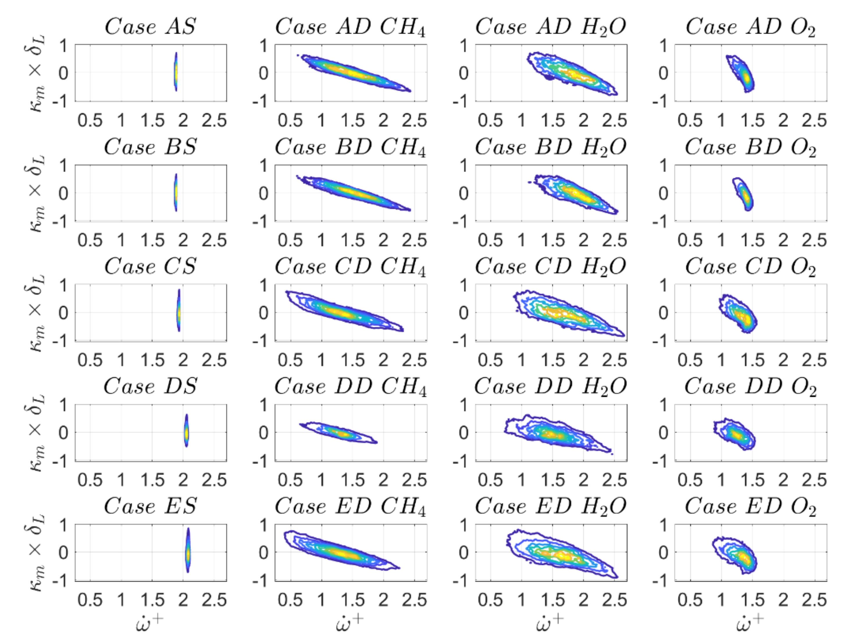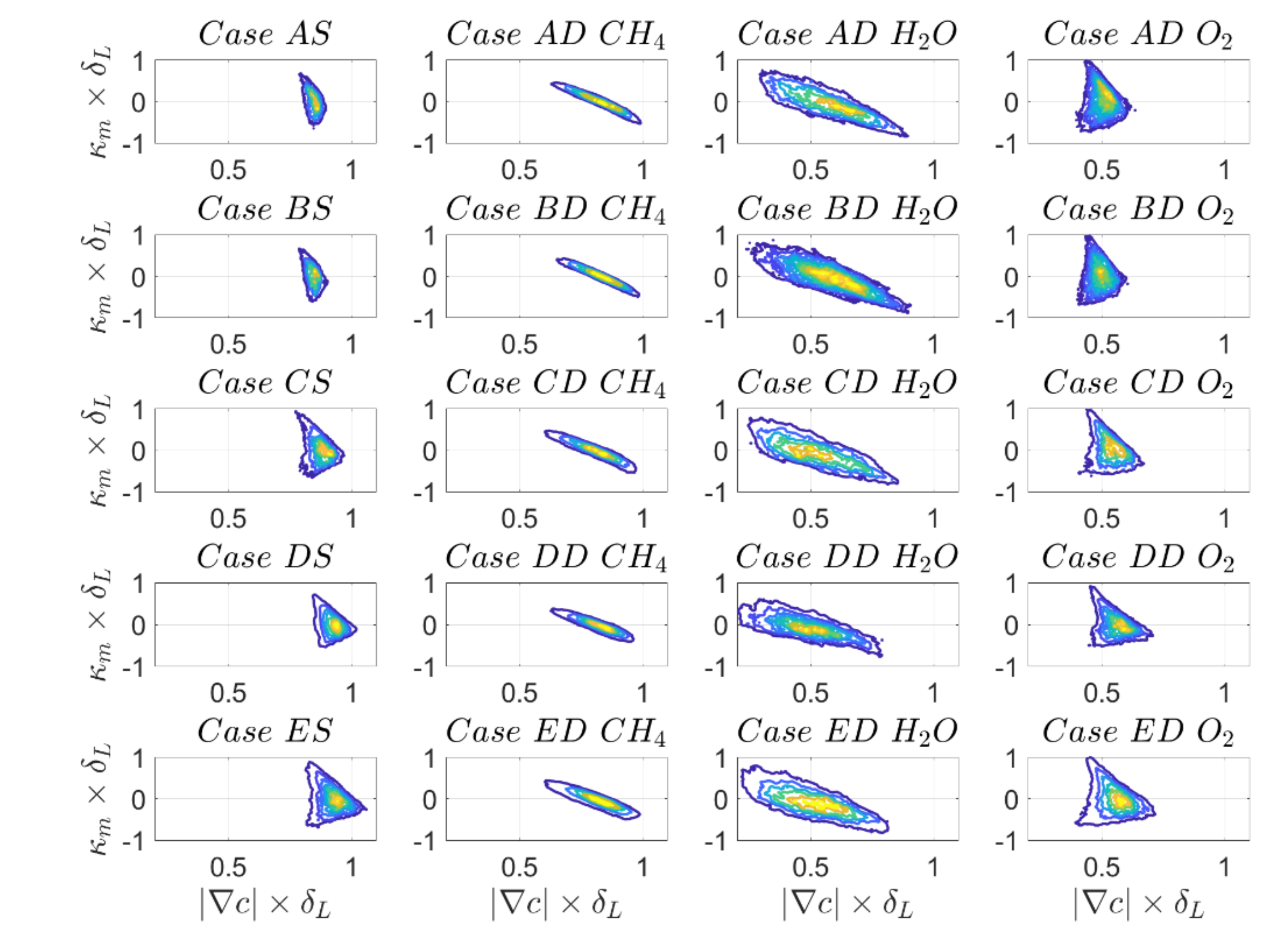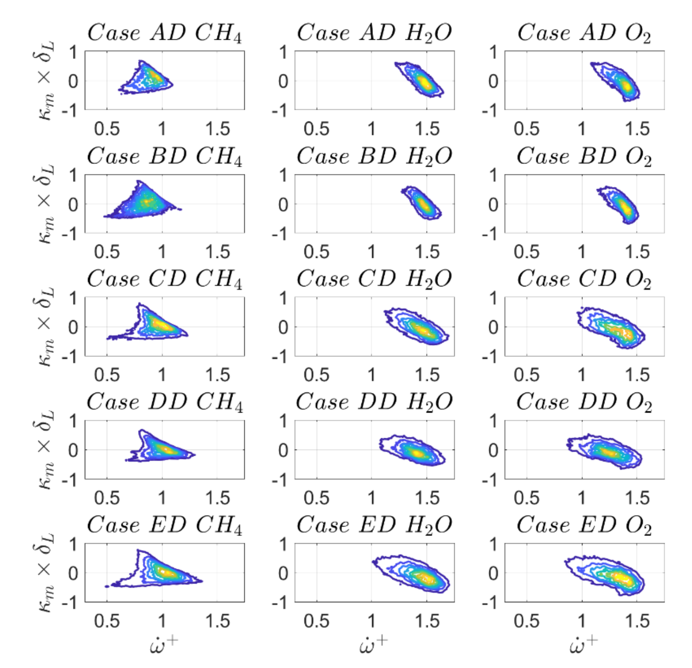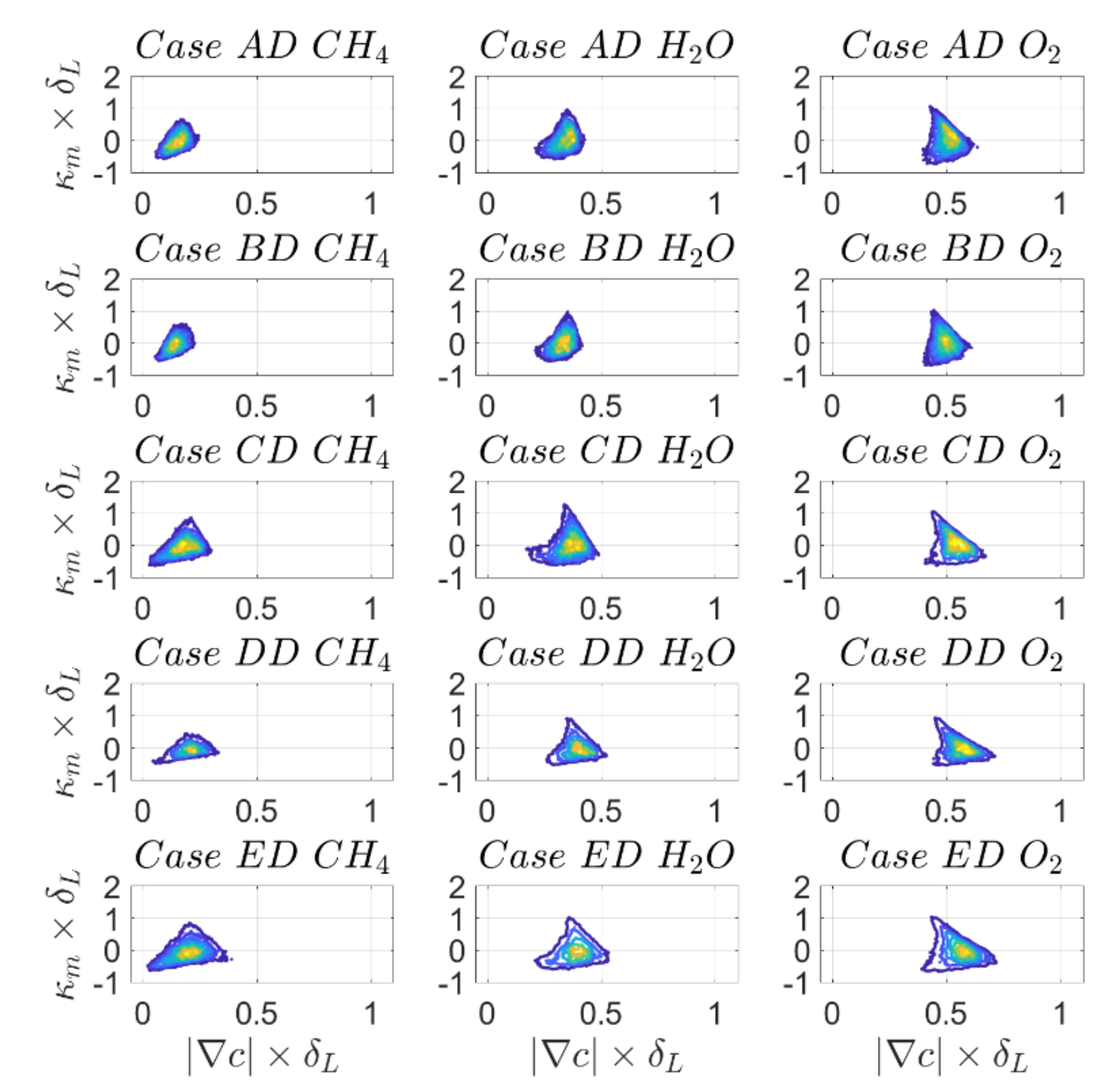Figure 17 and Figure 18 show the joint PDFs of normalised reaction rate $-\dot{\omega }\times {\delta }_L/\left[{\rho }_0{S}_L\left(Y_0-Y_{\infty }\right)\right]$ with mean curvature ${\kappa }_m$ and the joint PDFs for the surface density function $\left|\nabla c\right|$ with ${\kappa }_m$ on the $c=0.8$ isosurface, while the correlation coefficients are reported in

Table 12. Correlation coefficients between ${\dot{\omega }}^{+}$ and $\left|\nabla c\right|$ with ${\kappa }_m$ for the $c=0.8$ isosurface value for all cases.

	$\mathit{c}\mathit{o}\mathit{r}\mathit{r}\left({\dot{\mathit{\omega }}}^{\mathbf{+}}\mathbf{,}{\mathit{\kappa }}_{\mathit{m}}\right)$				$\mathit{c}\mathit{o}\mathit{r}\mathit{r}\left(\left|\mathbf{\nabla }\mathit{c}\right|\mathbf{,}{\mathit{\kappa }}_{\mathit{m}}\right)$
Case	SC	$\mathbf{DC} \mathbf{C}{\mathbf{H}}_{\mathbf{4}}$	$\mathbf{DC} {\mathbf{H}}_{\mathbf{2}}\mathbf{O}$	DC ${\mathbf{O}}_{\mathbf{2}}$	SC	$\mathbf{DC} \mathbf{C}{\mathbf{H}}_{\mathbf{4}}$	$\mathbf{DC} {\mathbf{H}}_{\mathbf{2}}\mathbf{O}$	DC ${\mathbf{O}}_{\mathbf{2}}$
A	0.02	−0.87	−0.83	−0.61	−0.29	−0.85	−0.78	−0.03
B	0.02	−0.86	−0.83	−0.57	−0.26	−0.83	−0.77	−0.01
C	0.02	−0.84	−0.77	−0.65	−0.15	−0.81	−0.74	−0.12
D	0.02	−0.77	−0.68	−0.62	−0.27	−0.71	−0.67	−0.18
E	0.03	−0.80	−0.72	−0.62	−0.18	−0.73	−0.69	−0.15

. For the ease of notation, the dimensionless reaction rate $-\dot{\omega }\times {\delta }_L/[{\rho }_0{S}_L\left(Y_0-Y_{\infty }\right)]$ will be referred to as ${\dot{\omega }}^{+}$ in the following. Indeed Figure 17 shows that $corr\left( {\dot{\omega }}^{+},{\kappa }_m\right)=0$ in the case of SC. Together with $corr\left(\left|\nabla c\right|,{\kappa }_m\right)\le 0$, this results in $corr\left(S_r,{\kappa }_m\right)\ge 0$. It is noted that for low Mach number and unity Lewis number flames density is constant on a given $c$ isosurface.

For DC, Figure 17 clearly indicates a negative correlation between reaction rate and curvature for all definitions of reaction progress variable on the $c=0.8$ isosurface. In the case of SC, this would correspond to a scenario with Lewis number larger than unity [31,32] while the opposite would be expected for $Le<1$. Indeed, it was discussed in the introduction that a methane flame is characterised by a Lewis number slightly larger than $1.0$ according to the parameterisations given by Equations (5)–(7) [45,46,47] which is qualitatively consistent with the trends shown in Figure 17. However, the species ${\mathrm{CH}}_4,{\mathrm{H}}_2\mathrm{O}$ and ${\mathrm{O}}_2$ have considerably different Lewis numbers ($Le=0.97,0.83,1.11$ respectively, according to Table 3) and therefore their behaviours warrant a more detailed discussion.

In $Le<1$ SC simulations [31,32], the focusing of reactants takes place at a faster rate than the rate of defocusing of heat at the positively curved zones, which leads to the simultaneous presence of high temperature and reactant concentrations and conversely for negatively curved regions. Hence, high (low) temperature values are associated with positive (negative) curvatures for $Le<1$ and the opposite is valid for $Le>1$ [27,28,29,30,31,32]. For the SC simulations, the reaction rate depends on temperature according to

$$\dot{{\omega }_c}=B^{*}\rho \left(1-c\right)\mathit{exp}\left(-\frac{E_{\mathit{act}}}{R^{0}T}\right)=\rho \left(1-c\right)k_f,{ k}_f=B^{*}\mathit{exp}\left(-\frac{E_{\mathit{act}}}{R^{0}T}\right)$$

(9)

where $B^{*}$ is the normalised pre-exponential factor, $E_{act}$is the activation energy, such that a negative (positive) correlation between$T$ and ${\kappa }_m$ induces a negative (positive) correlation between $\dot{\omega }$and ${\kappa }_m$ and the same holds true for non-dimensional temperature which will be denoted $T^{+}$ in the following discussion and in fact is identical to $c_T$. For a reaction mechanism involving $M$steps and $N$ species given by:

$${\displaystyle \sum }_{\alpha =1}^N{\nu }_{\alpha ,\beta }^{’}{X}_{\alpha } \iff {\displaystyle \sum }_{\alpha =1}^N{\nu }_{\alpha ,\beta }^{’’}{X}_{\alpha }, \beta =1,\dots ,M$$

(10)

the situation is much more complex and one obtains

$${\omega }_{\alpha }=M_{\alpha }{\displaystyle \sum }_{\beta =1}^M\left({\nu }_{\alpha ,\beta }^{″}-{\nu }_{\alpha ,\beta }^{’}\right)\left(r_{f,\beta }-r_{b,\beta }\right),{ r}_{f,\beta }-r_{b,\beta }=k_{f,\beta }{\displaystyle \prod }_{\alpha =1}^N{c}_{\alpha }^{{\nu }_{\alpha ,\beta }^{’}}-k_{b,\beta }{\displaystyle \prod }_{\alpha =1}^N{c}_{\alpha }^{{\nu }_{\alpha ,\beta }^{″}}$$

(11)

where the specific forward $\left(f\right)$ and backward $\left(b\right)$ reaction rate coefficients $k_{f/b,\beta }$ are given by an Arrhenius expression similar to Equation (9). Here, the ${\nu }_{\alpha ,\beta }^{’},{\nu }_{\alpha ,\beta }^{″}$ are called stoichiometric coefficients, $X_{\alpha }$ denotes the $N$ different species, $M_{\alpha }$ are the molar masses, $c_{\alpha }$the molar densities. Equation (11) shows that the reaction rate for species $\alpha$ in the context of DC depends on many more factors compared to the SC 1-step case shown in Equation (9) such that a negative (positive) correlation between $T^{+}$ and ${\kappa }_m$ does not necessarily induce a correlation of same sign between ${\dot{\omega }}_c$and ${\kappa }_m$. 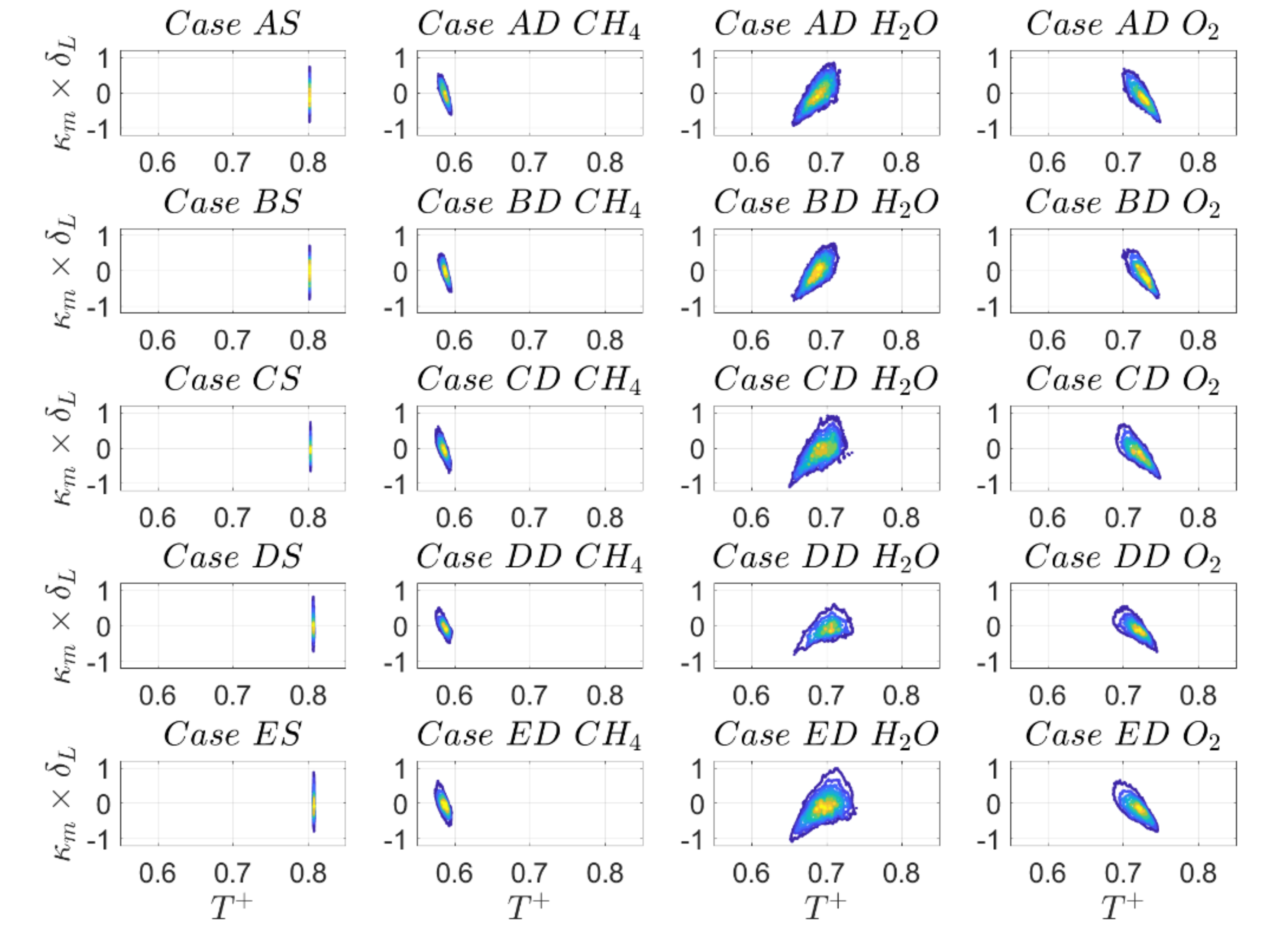A similar conclusion holds for ${\dot{\omega }}_T$ given by ${\dot{\omega }}_T=-{\displaystyle \sum }_{\alpha =1}^N{\dot{\omega }}_{\alpha }{h}_{\mathrm{f},\alpha }^0.$ A large reaction rate $\dot{{\omega }_{\alpha }}$ of species $\alpha$ does not necessarily imply a high ${\dot{\omega }}_T$ because the enthalpy of formation of species $\alpha$ can be very small or even zero. Finally, all species share the identical temperature field, such that explanations holding true for SC cannot directly be applied to DC without caution. In fact, the joint PDFs between temperature and curvature for the $c=0.8$ isosurface are shown in Figure 19 and the correlation coefficients are reported in

Table 13. Correlation coefficients between $T^{+}$ and ${\kappa }_m$ for the $c=0.8$ isosurface value for all cases.

	$\mathit{c}\mathit{o}\mathit{r}\mathit{r}\left({\mathit{T}}^{\mathbf{+}}\mathbf{,}{\mathit{\kappa }}_{\mathit{m}}\right)$
Case	SC	$\mathbf{DC} \mathbf{C}{\mathbf{H}}_{\mathbf{4}}$	$\mathbf{DC} {\mathbf{H}}_{\mathbf{2}}\mathbf{O}$	DC ${\mathbf{O}}_{\mathbf{2}}$
A	0.01	−0.20	0.59	−0.73
B	0.01	−0.19	0.58	−0.72
C	0.02	−0.21	0.52	−0.71
D	0.01	−0.18	0.43	−0.64
E	0.01	−0.19	0.45	−0.66

for the $c=0.8$ isosurface. Indeed, by comparing Figure 17 and Figure 19, it becomes obvious that $corr\left(T^{+},{\kappa }_m\right)>0$ while $corr\left({\dot{\omega }}^{+},{\kappa }_m\right)<0$ for reaction progress variable based on ${\mathrm{H}}_2\mathrm{O}$ mass fraction, indicating that the value of temperature and rate of formation of species $\alpha$ can be partially decoupled.

Water vapour is characterised by a higher diffusivity and Lewis number $Le=0.83$ (see Table 3). For SC the thermo-diffusive mechanisms explained before lead to higher reaction rates in positively curved regions and higher flame wrinkling for $Le<1$compared to $Le=1$ flames. As a result of this, positively (negatively) curved regions propagate faster (slower) and finger-like structures start to develop. A transfer of this mechanism to isosurfaces of individual $Le<1$ species in DC simulations is obviously not possible because all species transport equations are coupled. By contrast, as discussed next, it appears that the flame wrinkling of the ${\mathrm{H}}_2\mathrm{O}$ mass fraction-based reaction progress variable isosurface is smaller compared to those based on ${\mathrm{CH}}_4$ and ${\mathrm{O}}_2$ isosurfaces. This is a result of preferential diffusion and its influence on intermediate reaction steps and can on one hand be attributed to higher diffusivity of ${\mathrm{H}}_2\mathrm{O}$ which smoothens high curvature magnitudes. On the other hand, this effect is further attenuated by higher (reduced) reactivity in the positively (negatively) curved regions. The turbulent flame areas $A_T$ normalised by the cross-section of the computational domain $A_0$for ${\mathrm{CH}}_4,{\mathrm{H}}_2\mathrm{O}$ and ${\mathrm{O}}_2$ are exemplarily given by $A_T/A_0=1.553, 1.487$ and $1.557$ respectively for case A. The values for temperature isosurfaces (representing the laminar flame temperature for $c=0.8$) for the three definitions of reaction progress variable are given by $A_T/A_0=1.541, 1.516, 1.476$.

The reduced wrinkling of the ${\mathrm{H}}_2\mathrm{O}$ based reaction progress variable isosurface compared to ${\mathrm{O}}_2$ based reaction progress variable for case AD can be confirmed from Figure 20a, which shows a simultaneous plot of isosurfaces of reaction progress variable $c=0.8$ for ${\mathrm{H}}_2\mathrm{O}$ (red) and ${\mathrm{O}}_2$ (grey) with the ${\mathrm{O}}_2$ based isosurface overlapping the ${\mathrm{H}}_2\mathrm{O}$-based isosurface. Similar observations in terms of flame wrinkling have been reported for detailed chemistry hydrogen-air simulations [22]. 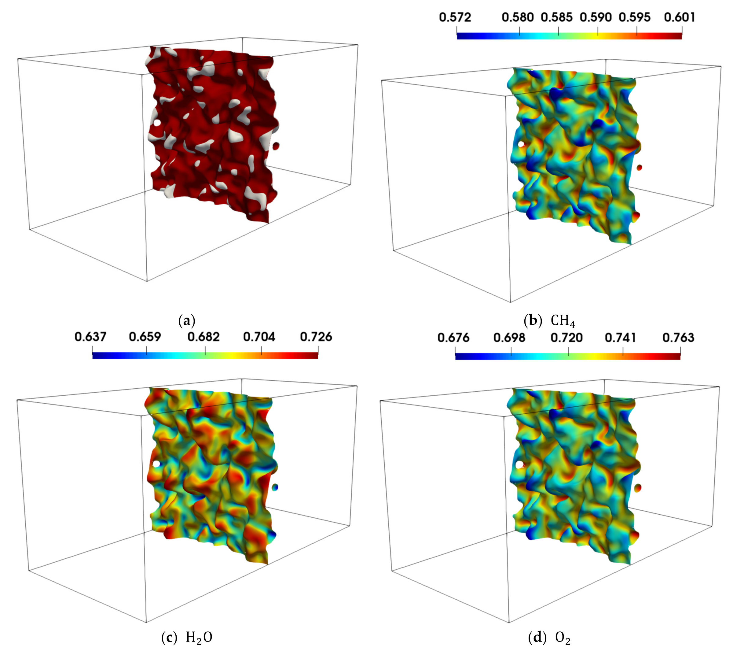Figure 20 also shows isosurfaces of $c=0.8$ coloured with non-dimensional temperature for case AD for reaction progress variable based on ${\mathrm{CH}}_4,{\mathrm{H}}_2\mathrm{O}$ and ${\mathrm{O}}_2$ mass fractions. The opposite correlation of temperature and curvature (observed in Figure 19) between ${\mathrm{CH}}_4$,${\mathrm{O}}_2$ and ${\mathrm{H}}_2\mathrm{O}$ can be clearly seen. While positively curved regions are characterised by lower temperature in the case of ${\mathrm{CH}}_4$ and ${\mathrm{O}}_2$ based reaction progress variable isosurfaces, they show higher temperature for ${\mathrm{H}}_2\mathrm{O}$. In order to understand this apparent contradiction, it is also important to recall that the different isosurfaces are characterised by different positions in the flame (see Figure 2 and Figure 3) and to note that the colour bars have different temperature ranges. As the ${\mathrm{H}}_2\mathrm{O}$ isosurface is less wrinkled than the corresponding temperature isosurface (because of higher mass diffusivity than thermal diffusivity), positively curved regions reach out less into to unburned gas side and hence they are characterised by higher temperatures. Similarly, negatively curved regions reach out less into the burned gas side and are consequently characterised by lower temperatures. The effect can be clearly seen in Figure 21a and is consistent with the positive correlation between $T$ and ${\kappa }_m$ for the ${\mathrm{H}}_2\mathrm{O}$-based reaction progress variable isosurface.

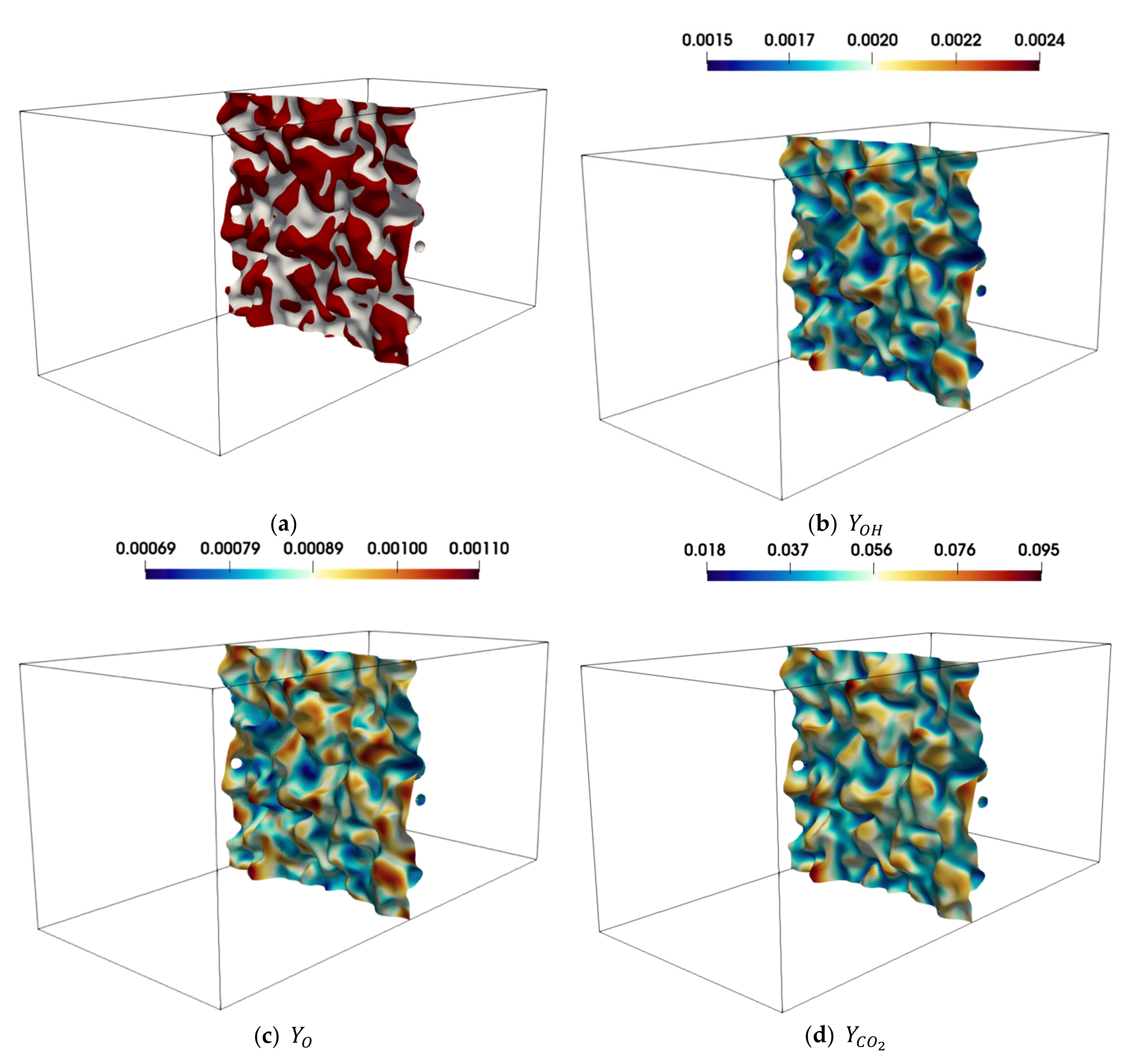
Besides diffusion, flame propagation and wrinkling are also determined by reactive effects. At the positively curved locations, focussing of $\mathrm{O} \left(Le=0.7\right)$ takes place at a faster rate than the defocussing of ${\mathrm{H}}_2\mathrm{O} \left(Le=0.83\right)$ and heat and this gives rise to a higher likelihood of the reaction $\mathrm{O}+{\mathrm{H}}_2\mathrm{O}\to \mathrm{OH}+\mathrm{OH}$ which is a chain propagation reaction and promotes heat release due to $\mathrm{CO}+\mathrm{OH}\to {\mathrm{CO}}_2+\mathrm{H}$. This also decreases the wrinkling of ${\mathrm{H}}_2\mathrm{O}$ based reaction progress variable isosurface at the positively curved locations, whereas just the opposite mechanisms lead to less wrinkling and smaller temperatures in the negatively curved locations. The higher concentrations of mass fractions $Y_{\mathrm{OH}},Y_{{\mathrm{CO}}_2}$ and $Y_{\mathrm{O}}$ in the positively curved regions of the $c=0.8$isosurface for ${\mathrm{H}}_2\mathrm{O}$ based reaction progress variable can be clearly seen in Figure 21b–d and support the above argument. A similar argument can be made to explain the increased wrinkling of the ${\mathrm{O}}_2$-based reaction progress variable isosurfaces and the negative correlation between temperature and curvature. The defocussing of $\mathrm{O}$ $\left(Le=0.7\right)$ and $\mathrm{OH}$ $\left(Le=0.73\right)$ takes place at faster rates than that of ${\mathrm{O}}_2$ at the positively curved locations. This acts to promote the forward reaction of the equilibrium reaction ${\mathrm{O}}_2+\mathrm{H}\leftrightarrow \mathrm{OH}+\mathrm{O}$ according to Le Chatelier. This can be substantiated from low concentrations of $\mathrm{H},\mathrm{OH}$ and $\mathrm{O}$ at the positively curved locations of $c=0.8$isosurface for ${\mathrm{O}}_2$-based reaction progress variable (not shown here).

In order to finally understand the joint PDFs of $S_r$ and ${\kappa }_m$, besides reaction rate, it is important to look at the joint PDFs of $\left|\nabla c\right|$ and ${\kappa }_m$. An initial observation from Figure 18 is that the joint PDFs for the ${\mathrm{O}}_2$-based reaction progress variable behave to some extent similar to the SC case (i.e., they show a small correlation magnitude with a positive and a negative correlating branch for negative and positive curvatures, respectively) while the joint PDFs for reaction progress variable based on ${\mathrm{CH}}_4$ and ${\mathrm{H}}_2\mathrm{O}$ mass fractions are negatively correlated and the positively correlating branch cannot be observed. It has been explained in part 1 of this paper that (for constant dilatation rate) $a_T$ and $a_n$ (where $a_n$ is the normal strain rate) are negatively correlated. Further, a compressive (negative) normal strain rate causes local thinning which acts to increase the scalar gradient $\left|\nabla c\right|$. The negative correlation between $a_T$ and ${\kappa }_m$ leads to the principally negative correlation between $\left|\nabla c\right|$ and ${\kappa }_m$. However, $\left|\nabla c\right|$ can also assume small values at locations of high negative curvature because of secondary thickening effects induced by high values of dilation rate, which locally overcomes $a_T$ to induce extensive normal strain rate (i.e., $a_N=\left(\partial u_i/\partial x_i-a_T\right)>0$) [44,50,51] leading to a positively correlating branch for SC and DC based on ${\mathrm{O}}_2$-based reaction progress variable definition.

Based on the correlation behaviour of numerator and denominator in the definition of $S_r$ and $S_n$, it is possible to infer the correlations of $S_r$ and $S_n$ with curvature. However, in contrast to low Mach number SC simulations where $\rho$ can be assumed to be constant on a given isosurface, the same assumption does not hold any longer in the case of DC simulations, such that the denominator $\rho \left|\nabla c\right|$ potentially shows a more complex behaviour than $\left|\nabla c\right|$ on its own (it is recalled that $\rho$ deterministically depends on $T$ such that different signs of $corr\left(\rho ,{\kappa }_m\right)$ can be observed for different reaction progress variable definitions, see Figure 19). The Pearson correlation coefficient between two random variables $x,y$ is given by the covariance of both variables divided by the product of their standard deviations: $corr\left(x,y\right)=cov\left(x,y\right)/\sigma \left(x\right)\sigma \left(y\right).$ For the sign of the correlation, it is sufficient to look at the covariance between the random variables. Following Bohrnstedt and Goldberger [52], the covariance of the product of two random variables $x,y$ with a third random variable $z$ is given by the expression $cov\left(xy,z\right)=E\left(x\right)cov\left(y,z\right)+E\left(y\right)cov\left(x,z\right)+\mathrm{TOM}$, where $E$ denotes the expected value of a variable and $\mathrm{TOM}$ is the third-order moment of the three variables. It can be shown that the third-order moment vanishes under multivariate normality. In the present case, it is not negligible. The above identity shows that

$$cov\left(S_r,{\kappa }_m\right)=E\left({\dot{\omega }}_c\right)cov\left({\left(\rho \left|\nabla c\right|\right)}^{-1},{\kappa }_m\right)+E\left({\left(\rho \left|\nabla c\right|\right)}^{-1}\right)cov\left({\dot{\omega }}_c,{\kappa }_m\right)+TOM$$

$$\mathrm{TOM}=E(\left[\dot{{\omega }_c}-\left(E\left({\dot{\omega }}_c\right)\right]\cdot \left[{\rho }^{-1}{\left|\nabla c\right|}^{-1}-E\left({\rho }^{-1}{\left|\nabla c\right|}^{-1}\right)\right]\cdot \left[{\kappa }_m-E\left({\kappa }_m\right)\right]\right).$$

(12)

In other words, the sign of the correlation $S_r-{\kappa }_m$ depends on the expected values of $\dot{{\omega }_c}$ and ${\left(\rho \left|\nabla c\right|\right)}^{-1}$ and the covariances of these variables with ${\kappa }_m$.

Table 14. Statistical quantities that influence the value of $cov\left(S_r,{\kappa }_m\right)$ (see Equation (12)) for the $c=0.8$ isosurfaces for all cases and reaction progress variable based on ${\mathrm{CH}}_4$ and ${\mathrm{H}}_{2}O.$.

$\mathbf{C}{\mathbf{H}}_{\mathbf{4}}$
Case	A	B	C	D	E
$E\left({\dot{\omega }}_c\right)$	2547.7839	2597.5061	2273.8599	2160.8817	2180.9715
$cov\left({\left(\rho \left|\nabla c\right|\right)}^{-1},{\kappa }_m\right)$	0.20433	0.18014	0.33019	0.34091	0.37618
$E\left({\left(\rho \left|\nabla c\right|\right)}^{-1}\right)$	0.0015329	0.0015269	0.0016150	0.0016129	0.0016302
$cov\left({\dot{\omega }}_c,{\kappa }_m\right)$	−751,187.00	−676,192.05	−919,408.02	−731,584.85	−954,295.71
TOM	−60.0990	−57.2640	−228.2253	−377.3336	−341.6941
$H_{\mathbf{2}}O$
Case	A	B	C	D	E
$E\left(\dot{{\omega }_c}\right)$	2237.9615	2289.0814	2053.1845	1881.6142	1954.8047
$cov\left({\left(\rho \left|\nabla c\right|\right)}^{-1},{\kappa }_m\right)$	1.02550	0.89893	1.59752	2.02497	2.10159
$E\left({\left(\rho \left|\nabla c\right|\right)}^{-1}\right)$	0.0038432	0.0037235	0.0043388	0.0049527	0.0046655
$cov\left(\dot{{\omega }_c},{\kappa }_m\right)$	−408,617.71	−363,331.63	−532,049.84	−449,955.47	−568,270.69
TOM	−245.1527	−274.8800	−516.1845	−1037.0266	−1090.5936

and

Table 15. Statistical quantities that influence the value of $cov\left(S_n,{\kappa }_m\right)$ (see Equation (12)) for the $c=0.8$ isosurfaces for all cases and reaction progress variable based on ${\mathrm{CH}}_4$ and ${\mathrm{H}}_2\mathrm{O}$ mass fractions. The normal diffusion contribution is abbreviated as $D_n=\overrightarrow{N}.\nabla \left(\rho D_c \overrightarrow{N}.\nabla c\right)$.

$\mathbf{C}{\mathbf{H}}_{\mathbf{4}}$
Case	A	B	C	D	E
$E\left(D_n\right)$	−1187.524	−1173.584	−1075.307	−1145.738	−1103.740
$cov\left({\left(\rho \left|\nabla c\right|\right)}^{-1},{\kappa }_m\right)$	0.204331	0.180144	0.330189	0.340906	0.376177
$E\left({\left(\rho \left|\nabla c\right|\right)}^{-1}\right)$	0.0015329	0.0015269	0.0016150	0.0016129	0.0016302
$cov\left(D_n,{\kappa }_m\right)$	472,799.28	421,392.21	480,392.25	364,752.29	456,424.34
TOM	50.9848	44.8605	132.2754	180.1813	157.2711
${\mathbf{H}}_{\mathbf{2}}\mathbf{O}$
Case	A	B	C	D	E
$E\left(D_n\right)$	−1552.099	−1559.315	−1441.952	−1408.511	−1411.659
$cov\left({\left(\rho \left|\nabla c\right|\right)}^{-1},{\kappa }_m\right)$	1.025502	0.898930	1.597516	2.024971	2.101588
$E\left({\left(\rho \left|\nabla c\right|\right)}^{-1}\right)$	0.0038432	0.0037235	0.0043388	0.0049527	0.0046655
$cov\left(D_n,{\kappa }_m\right)$	272,601.83	236,782.06	319,153.43	279,084.77	326,451.96
TOM	234.3450	232.8878	580.4848	1070.1031	1077.2522

show the individual contributions of$cov\left(S_r,{\kappa }_m\right)$ and $cov\left(S_n,{\kappa }_m\right)$, respectively, according to Equation (12), exemplarily for reaction progress variable based on ${\mathrm{CH}}_4$ and ${\mathrm{H}}_2\mathrm{O}$. These species have been selected because they show similar correlations trends for ${\dot{\omega }}_c-{\kappa }_m$ and $\left|\nabla c\right|-{\kappa }_m$ but $corr\left(S_r,{\kappa }_m\right)$ shows the opposite sign for ${\mathrm{CH}}_4$ and ${\mathrm{H}}_2\mathrm{O}$, which requires additional explanation and a similar statement holds true for $corr\left(S_n,{\kappa }_m\right)$.

By referring to the terms in Equation (12), it can be seen from Table 14 that the higher magnitudes of $cov\left({\left(\rho \left|\nabla c\right|\right)}^{-1},{\kappa }_m\right)$ are mainly responsible for the change of sign of $cov\left(S_r,{\kappa }_m\right)$ in the case of ${\mathrm{H}}_2\mathrm{O}$ mass fraction-based reaction progress variable in comparison to ${\mathrm{CH}}_4$ mass fraction-based reaction progress variable. The change of sign of $cov\left({\left(\rho \left|\nabla c\right|\right)}^{-1},{\kappa }_m\right)$ in the case of ${\mathrm{H}}_2\mathrm{O}$-based reaction progress variable in comparison to ${\mathrm{CH}}_4$based reaction progress variable is the result of two effects. Firstly, the reaction progress variable based on ${\mathrm{H}}_2\mathrm{O}$ mass fraction has a small plateau for values slightly larger than ${\mathrm{c}}_{{\mathrm{H}}_2\mathrm{O}}=0.8$which results in small values of $\left|\nabla c\right|$ and hence large values of ${\left|\nabla c\right|}^{-1}$. Secondly, the positive correlation $T-{\kappa }_m$ induces a negative correlation $\rho -{\kappa }_m$ due to the ideal gas law. This, in turn, reinforces the negative correlation $\left|\nabla c\right|-{\kappa }_m$ for ${\mathrm{H}}_2\mathrm{O}$-based reaction progress variable, while it results in a change of sign and weakening of correlation strength for ${\mathrm{CH}}_4$-based reaction progress variable because of opposing correlations of $\rho$ and $\left|\nabla c\right|$ with ${\kappa }_m$. A similar explanation provides the explanations for the correlation behaviour between $S_n$ and ${\kappa }_m$ (see Table 15).

The foregoing discussion has shown that the statistics of $S_r, S_n$ and $\left|\nabla c\right|$ with curvature are sensitive to the definition of reaction progress variable and detailed explanations for this behaviour have been provided. Besides that, the statistics are also sensitive to the choice of isosurface level, which is also evident from the correlation coefficients reported in Table 11, Table 12 and Table 13. Important qualitative differences have also been found for the joint PDFs of normalised reaction rate, surface density function and non-dimensional temperature with mean curvature. These differences have been explained based on preferential diffusion and its influence on intermediate reaction steps which give rise to different degrees of wrinkling of different isosurfaces for different definitions of reaction progress variable.

For further illustration, the joint PDFs of normalised reaction rate, $\left|\nabla c\right|$, $S_r,$ and $S_n$ for different definitions of reaction progress variable are exemplarily shown in Figure A1, Figure A2, Figure A3 and Figure A4 in Appendix A, but in contrast to earlier figures, the statistics are now taken on the same isosurface corresponding to the ${\mathrm{O}}_2$ based reaction progress variable value of $c=0.8$. It can be seen from Figure A1, Figure A2, Figure A3 and Figure A4 in Appendix A that some of the qualitative differences observed earlier diminish if statistics are taken on the same ${\mathrm{O}}_2$ based reaction progress variable isosurface, and similar qualitative trends have been observed for other reaction progress variable definitions. For example, $corr\left(S_r,{\kappa }_m\right)$ becomes now consistently negative and, in addition, the negative correlation $corr\left(\left|\nabla c\right|,{\kappa }_m\right)$ vanishes.

4. Conclusions

Flame propagation statistics from three-dimensional simple chemistry and transport DNS have been compared to results obtained from detailed chemistry and transport simulations using a new database consisting of five simple chemistry (SC) and detailed chemistry and transport (DC) simulations of statistically planar turbulent premixed, stoichiometric methane-air flames for a range of different Damköhler, Karlovitz and turbulent Reynolds number values. Both methodologies use nearly identical numerical methods and the identical initial and boundary conditions. The discussion includes interdependencies of displacement speed and its individual components as well as surface density function and reaction rate with tangential strain rate and curvature using three different reaction progress variable definitions based on ${\mathrm{CH}}_4,{\mathrm{H}}_2\mathrm{O}$ and ${\mathrm{O}}_2$ mass fractions. The findings can be summarised as follows:

• The statistics of $S_d,\left(S_r+S_n\right),a_T,{\kappa }_m$ and their interrelation with each other remain qualitatively and to a large extent quantitatively similar for SC and DC and as well for different definitions of reaction progress variable.
• However, there are marked qualitative differences for individual contributions of displacement speed $S_r$ and $S_n$ and their interrelation with the curvature such that depending on the definition of reaction progress variable different signs of the correlation coefficient have been observed.
• Similar qualitative differences have also been found for the joint PDFs of normalised reaction rate ${\dot{\omega }}^{+}$, surface density function $\left|\nabla c\right|$ and non-dimensional temperature $T^{+}$ with mean curvature ${\kappa }_m$.
• These differences have been explained based on preferential diffusion and its influence on intermediate reaction steps which give rise to different extents of wrinkling of reaction progress variable isosurfaces for its different definitions. This leads to different correlations between temperature and mean curvature, which also induces different dependencies between density and mean curvature.
• In addition, the different variations of reaction progress variable $c$ across the flame for different definitions of reaction progress variable contribute to differences in $\left|\nabla c\right|$ variation. This may lead to small values of $\left|\nabla c\right|$ towards the burned gas side for some definitions of $c$, which results in a poorly conditioned definition of displacement speed and its components towards the product side.
• The reaction rate of some individual species $\alpha$ can be decoupled from temperature or ${\omega }_T$ while their interrelation is much more straightforward for a 1-step simplified chemical reaction. While for SC, reaction rate and density can be considered independent of mean curvature for unity Lewis number, adiabatic low Mach number simulations, this simplification does not hold true for detailed chemistry and transport.

Without any doubt, DC simulations provide more detailed information about the flame structure than SC simulations. However, the choice of reaction progress variable together with a suitable isosurface value gives rise to considerable uncertainty in the interpretation of displacement speed statistics, sometimes even showing opposing trends. Single-step chemistry simulations are shown to capture the correct qualitative trends of flame propagation statistics and do not have uncertainties with respect to the choice of reaction progress variable. Therefore, SC simulation results are more straightforward to compare with theoretical analysis or model assumptions, which are usually based on SC assumptions. The present results illustrate the advantages and disadvantages of both SC and DC simulations and aim to help combustion researchers to balance computational cost and associated carbon dioxide emissions with accuracy requirements. Moreover, the advantages of having lots of detailed information in DC needs to be contrasted with the possibility of having a large parametric study or a larger scale separation in SC.

Finally, this work is limited to the flames with an effective Lewis number close to unity. Extending the comparison to different Lewis numbers, together with the identification of suitable definitions for global Lewis number of more complex or dual fuel mixtures is part of the future work.