Analysis of Local Exergy Losses in Combustion Systems Using a Hybrid Filtered Eulerian Stochastic Field Coupled with Detailed Chemistry Tabulation: Cases of Flames D and E

Abstract

A second law analysis in combustion systems is performed along with an exergy loss study by quantifying the entropy generation sources using, for the first time, three different approaches: a classical-thermodynamics-based approach, a novel turbulence-based method and a look-up-table-based approach, respectively. The numerical computation is based on a hybrid filtered Eulerian stochastic field (ESF) method coupled with tabulated detailed chemistry according to a Famelet-Generated Manifold (FGM)-based combustion model. In this work, the capability of the three approaches to capture the effect of the Re number on local exergy losses is especially appraised. For this purpose, Sandia flames D and E are selected as application cases. First, the validation of the computed flow and scalar fields is achieved by comparison to available experimental data. For both flames, the flow field results for eight stochastic fields and the associated scalar fields show an excellent agreement. The ESF method reproduces all major features of the flames at a lower numerical cost. Next, the second law analysis carried out with the different approaches for the entropy generation computation provides comparable quantitative results. Using flame D as a reference, for which some results with the thermodynamic-based approach exist in the literature, it turns out that, among the sources of exergy loss, the heat transfer and the chemical reaction emerge notably as the main culprits for entropy production, causing 50% and 35% of it, respectively. This fact-finding increases in Sandia flame E, which features a high Re number compared to Sandia flame D. The computational cost is less once the entropy generation analysis is carried out by using the Large Eddy Simulation (LES) hybrid ESF/FGM approach together with the look-up-table-based or turbulence-based approach.

1. Introduction

Most energy conversion systems feature, typically, 20–30% of exergy destruction in fuel combustion [1]. In searching for more exergy-efficient combustion, the evaluation of the second law efficiency and subsequent analysis of local entropy generation consisting of minimizing the irreversibilities can be used to optimize the efficiency of current and future systems of energy conversion [1,2,3,4,5]. Previous studies provide reviews of the fundamentals of second-law-based analysis [1,2,3,4,5]. These comprise system-level analysis, commonly called exergy analysis, to calculate the net rate of energy degradation. Thereby, most contributions deal with thermal devices in which viscous and thermal effects for convective heat transfer [3], as well as combined mass and heat transfer phenomena [3], play a significant role. Investigations on entropy analysis in combustion systems are very scarce. Sources of irreversibilites may include heat transfer, mechanical dissipation, mass transfer and diffusion, chemical reactions, phase change, inelastic material deformation and breakup, etc. [1,2,3,4,5,6]. Such irreversibilities lead to a destruction of available energy into internal energy in the system, which causes a raise in the system entropy [1,2,3,4]. This rising of entropy, known as entropy generation/production, results in an abatement of the thermodynamic performance of the system.

The objective of the entropy generation analysis is threefold. First, it requires the formulation of appropriate models that describe the evolving transport processes, taking into account the finite size of actual systems and the finite speeds of ongoing real processes. Second, it allows not only the identification of the causes of inefficiency of processes but also permits the evaluation of the significance (location and magnitude) of irreversibilities generated by each specific transport process. Third, it aids to delimit the evolution of the processes, and at the same time gives access to the control and possible minimization of irreversibilities.

The present paper focuses on the second aspect by assuming that models that describe the evolving transport processes in combustion systems are available. Dealing with turbulent flows, a large eddy simulation (LES) approach is adopted as a modeling approach due to its obvious advantages. In fact, large, unsteady turbulent motions are explicitly simulated by LES, while a so-called sub-grid scale (SGS) closure model accounts for the influence of non-resolved SGS structures. Compared to direct numerical simulation in which all the turbulent structures are resolved, LES allows affordable computational efforts and improves the predictive capability of RANS (Reynolds-Averaged Navier–Stokes or Reynolds-Averaged Numerical Simulation), in which all or the most turbulent motions are averaged. Nevertheless, Entropy Generation Analysis (EGA) using LES is very rare, surely due to the difficulties in fairly modeling the non-resolved SGS production rates of entropy.

Recently, the research group at TU Darmstadt published a series of contributions dealing with EGA by using LES for various non-reacting flow and heat transfer applications, see in Ries et al. [7,8,9,10]. In reacting environments, Safari et al. [11,12] were the first to employ LES in dealing with EGA. They proposed and used an approach which relies on a transport equation of the Filtered Density Function (FDF). This methodology is known to provide the chemical source term in a closed form [13,14]. In addition to the classical filtered balance equations of mass, momentum, energy and species mass fractions, this so-called entropy FDF approach (En-FDF) includes a filtered transport equation for the entropy. Such an En-FDF approach comprises in a comprehensive manner the statistical information about the scalar, velocity, turbulent frequency and entropy fields, and thus allows the formulation of SGS closures for all the non-closed moments in the filtered governing equations. It enables accurate predictions of appearing non-resolved entropy generation in simple turbulent reacting flows, including Sandia flame D. However, it is costly and cannot, in this form, be utilized as a straightforward post-processing tool in a commercial CFD code. Alternative analysis using LES for reacting flows that include the SGS contributions of the entropy generation are not yet available in the literature. Table 1 summarizes the main recent studies on entropy production in combustion systems.

To alleviate the computational expenses related to En-FDF modeling, a new approach is proposed in the present paper. Within a LES framework this solves a Transported Filtered Density Function (T-FDF) following the Eulerian Stochastic Field methodology (ESF) coupled with a detailed chemistry tabulation according to the flamelet-generated manifold (FGM) strategy. This results in the so-called LES hybrid filtered ESF/FGM approach which can be well applied to combustion systems featuring various combustion regimes (premixed, non-premixed, mixed or multimode). Since the chemical source term is closed in this approach, the combustion and the involved Turbulence–Chemistry Interaction (TCI) can be described in an accurate way, taking advantage of tabulated chemistry. Thereby, it is possible to easily account for the effects of SGS entropy production by means of various methods without consideration of additional filtered transport equations. This feature makes the suggested methodology computationally affordable and suitable for use as a simple post-processing tool. It is worth mentioning that the methodology copes well with existing SGS models that describe the flow and thermal field within existing academic and even commercial CFD codes.

In energy systems working under a non-premixed combustion mode (e.g., glass furnaces, rocket engines or gas turbines under particular operating conditions, etc.), an oxidizer and fuel enter the reaction zone in different streams, and rapid mixing is required to increase the heat release rates. Even though they are easy to design and safe to operate, these kinds of systems are highly pollutant and less efficient compared to premixed burners, in which reactants are already mixed at the molecular level before burning. Furthermore, they exhibit strong interactions between turbulent fluctuations and chemical reactions, which necessitate advanced prediction tools in order to be analyzed in a better fashion, allowing better control and optimization. For laminar cases Nishida et al. [1] reported that a chemical reaction is the predominant process for exergy destruction in laminar premixed flames, while heat conduction is rather dominant in diffusion flames. The question is now to investigate these aspects under turbulent operating conditions using LES.

To reduce the modeling complexity of resolving the flame front on a LES mesh related to premixed flames, we restrict ourself in the present paper to the application of the suggested methodology to non-premixed combustion systems, especially to Sandia flames D and E that belong to the Sandia flame series D–F. The two flames feature different combustion characteristics including very little local extinction (flame D close to equilibrium) and high global extinction (flame E far from equilibrium) with an increased Re number. These flames have been already investigated using the transported FDF approach using the Lagrangian procedure in [13,14] or the Eulerian stochastic field in [15,16,17]. Up to now, a transported FDF approach relying on an Eulerian stochastic field that deals with entropy generation analysis is not yet available in the literature.

The objective of the present paper is therefore threefold: (a) to carry out EGA by applying the hybrid filtered Eulerian stochastic field (ESF) method coupled with the FGM chemistry tabulation strategy; (b) to suggest two novel methods for quantifying entropy generation sources in addition to the classical-thermodynamics-based one; (c) to assess the capability of the novel approaches to capture the effect of the Re number on local exergy losses in terms of accuracy and computational costs.

The present paper is organized as follows. In Section 2 the modeling methodology including the LES description, the tabulated chemistry strategy and the exergy analysis framework is briefly outlined. In Section 3, the two different flame cases under study are introduced, and validation results are then provided and discussed. Subsequently, detailed exergy analysis in both investigated cases is presented in Section 4. Section 5 is dedicated to conclusions.

Table 1. Recent investigations on analysis of Entropy Generation (EG) applied to combustion systems.

Authors	Simulation	Fuel, Fuel Mixture	Configuration and Working Parameters	Main Outcomes
Safari, M. et al. [12]	Three-dimensional numerical	Methane	Non-premixed flame	Heat transfer and chemical reaction are the main culprits of EG
Nishida, K. et al. [1]	Three-dimensional numerical	Methane/hydrogen	Non-premixed and premixed flames	Heat transfer is the major source of EG in diffusion flame
Jejurkar and Mishra [18]	Three-dimensional numerical	Hydrogen	Multi-step kinetics on annular combustor	EG rate rises from lean to rich mixture (0.5 < Φ < 1.4)
Wenming et al. [19]	Numerical and experimental	Hydrogen	Gap length of block insert	Combustor with a gap length of 4 mm causes the lowest EG rate. Higher gap length results in higher EG
Morsli et al. [20]	Two-dimensional numerical	Propane	Oxygen percentage in air, equivalence ratio and inlet velocity	Thermal effect provides the main contribution to the total EG
Safer et al. [21]	Numerical	Hydrogen/carbon monoxide	Counterflow flames of syngas mixtures	Total volumetric EG decreases with hydrogen enrichment
Mohammadi and Ajam [22]	Two-dimensional numerical	Methane	Multi-step mechanisms and variable porosity of porous media	Heat transfer has the highest contribution in EG rate
Zuo et al. [23]	Three-dimensional numerical	Hydrogen	Mass flow rate, equivalence ratio, materials and inlet/outlet diameter ratios of variant diameter chambers	Modified microreactor features lower total EG compared to the old microreactor
Ni et al. [24]	Three-dimensional numerical	Hydrogen	Axial location and height of geometric shape ribs	Chemical reaction and conduction heat transfer contribute up to 70% and 15% of the total EG, respectively
Ansari and Amani [25]	Three-dimensional numerical	Methane	Flame stability, efficiencies and emission on combined baffle-bluff	In both combustion and MTPV efficiency, the EG rate is reduced by increasing the solid wall conductivity
Wang et al. [26]	Numerical	Methane/hydrogen addition	Flow velocity and H2 addition in a micro-planar combustor	EG rate induced by chemical reaction, mass diffusion and heat conduction rises with the flow velocity
Prashant et al. [27]	One-dimensional numerical	Hydrogen	Wall permeability, fuel–air ratio and unburnt mixture temperature	Fuel permeation through the wall tends to decrease the EG per unit of converted fuel

Table 1. Recent investigations on analysis of Entropy Generation (EG) applied to combustion systems.

Authors	Simulation	Fuel, Fuel Mixture	Configuration and Working Parameters	Main Outcomes
Safari, M. et al. [12]	Three-dimensional numerical	Methane	Non-premixed flame	Heat transfer and chemical reaction are the main culprits of EG
Nishida, K. et al. [1]	Three-dimensional numerical	Methane/hydrogen	Non-premixed and premixed flames	Heat transfer is the major source of EG in diffusion flame
Jejurkar and Mishra [18]	Three-dimensional numerical	Hydrogen	Multi-step kinetics on annular combustor	EG rate rises from lean to rich mixture (0.5 < Φ < 1.4)
Wenming et al. [19]	Numerical and experimental	Hydrogen	Gap length of block insert	Combustor with a gap length of 4 mm causes the lowest EG rate. Higher gap length results in higher EG
Morsli et al. [20]	Two-dimensional numerical	Propane	Oxygen percentage in air, equivalence ratio and inlet velocity	Thermal effect provides the main contribution to the total EG
Safer et al. [21]	Numerical	Hydrogen/carbon monoxide	Counterflow flames of syngas mixtures	Total volumetric EG decreases with hydrogen enrichment
Mohammadi and Ajam [22]	Two-dimensional numerical	Methane	Multi-step mechanisms and variable porosity of porous media	Heat transfer has the highest contribution in EG rate
Zuo et al. [23]	Three-dimensional numerical	Hydrogen	Mass flow rate, equivalence ratio, materials and inlet/outlet diameter ratios of variant diameter chambers	Modified microreactor features lower total EG compared to the old microreactor
Ni et al. [24]	Three-dimensional numerical	Hydrogen	Axial location and height of geometric shape ribs	Chemical reaction and conduction heat transfer contribute up to 70% and 15% of the total EG, respectively
Ansari and Amani [25]	Three-dimensional numerical	Methane	Flame stability, efficiencies and emission on combined baffle-bluff	In both combustion and MTPV efficiency, the EG rate is reduced by increasing the solid wall conductivity
Wang et al. [26]	Numerical	Methane/hydrogen addition	Flow velocity and H2 addition in a micro-planar combustor	EG rate induced by chemical reaction, mass diffusion and heat conduction rises with the flow velocity
Prashant et al. [27]	One-dimensional numerical	Hydrogen	Wall permeability, fuel–air ratio and unburnt mixture temperature	Fuel permeation through the wall tends to decrease the EG per unit of converted fuel

2. Modeling Approach

In this section, two main modeling levels are introduced. The first addresses the LES hybrid ESF/FGM approach adopted. The second focuses on the exergetic analysis framework in which different methods for quantifying the entropy generation rates in single-phase turbulent reacting flows are outlined.

2.1. The LES Hybrid ESF/FGM Approach

The adopted LES hybrid ESF/FGM approach utilizes LES modeling and couples a Transported joint scalar Filtered Density Function (T-FDF), following the ESF methodology, with the tabulated detailed chemistry strategy according to the FGM-based combustion model.

2.1.1. LES Description and FGM Tabulated-Chemistry-Based Combustion Model

As pointed out in the introduction, depending upon the finite size of actual systems and the finite speeds of evolving real processes, many sources of irreversibilities of multicomponent flow can be encountered in combustion systems fired by gaseous fuels. For non-confined systems, these may include heat conduction, mass diffusion, viscous dissipation and chemical reactions [1,6]. To better account for the contribution of chemical reactions, detailed chemistry shall be considered [1,11,12]. Under turbulent conditions, the turbulence–chemistry interaction process must also be well-captured.

To consider detailed chemistry within the LES framework, an effort has been made to reduce the overall computational cost by suggesting, in particular, various chemical mechanism reductions as well as chemistry tabulation or storage approaches as reported in [28,29,30,31,32]. In the present study, the Flamelet-Generated Manifold (FGM) is adopted as one of the most promising reduction strategies. It makes it possible to describe detailed chemistry with only a few control parameters.

In the present work, the mixture fraction, Z, introduced according to Bilger et al. [33], and the progress variable, Y_c, are considered as the controlling variables. The progress variable, Y_c, is defined as [34]:

$$Y_c=\frac{Y_{C{O}_2}}{M_{C{O}_2}}+\frac{Y_{CO}}{M_{CO}}+\frac{Y_{H_{2}O}}{M_{H_{2}O}}$$

(1)

where M stands for the molar mass and Y the mass fraction. By means of a laminar diffusion counterflow flame solver, the Cantera code [35], a 2D manifold is generated. The chemical mechanism employed contains 325 reactions and 53 species as available in Gri-Mech 3.0. A set of one-dimensional diffusion flamelets is then simulated with an increasing strain rate under a unity Lewis number assumption until the flamelet is extinguished. These flamelets are afterwards collected in the same database, referred to as two-dimensional FGM manifold. In this so-called look-up table, various key thermo-chemical quantities, such as chemical source term, temperature, density, viscosity and species mass fraction, etc., are stored.

Coupling the FGM method with LES, the filtered transport equations for the control variables (Equations (4) and (5)) are solved together with the classical filtered transport equations for mass density (Equation (2)) and momentum (Equation (3)). This yields the following set of equations:

$$\frac{\partial \overline{\rho }}{\partial t}+\frac{\partial \overline{\rho }{\tilde{u}}_i}{\partial x_i}=0$$

(2)

$$\frac{\partial \overline{\rho }{\tilde{u}}_i}{\partial t}+\frac{\partial \overline{\rho }{\tilde{u}}_i{\tilde{u}}_j}{\partial x_j}=-\frac{\partial \overline{p}}{\partial x_i}+\frac{\partial }{\partial x_j}\left[\overline{\mu }\left(\frac{\partial {\tilde{u}}_i}{\partial x_j}+\frac{\partial {\tilde{u}}_j}{\partial x_i}-\frac{2}{3}\frac{\partial {\tilde{u}}_k}{\partial x_k}{\delta }_{ij}\right)\right]\_\frac{\partial }{\partial x_j}\left(\overline{\rho }{\tau }_{ij}^{sgs}\right)$$

(3)

$$\frac{\partial \overline{\rho }\tilde{Z}}{\partial t}+\frac{\partial \overline{\rho }{\tilde{u}}_j\tilde{Z}}{\partial x_j}=\frac{\partial }{\partial x_j}\left[\left(\frac{\overline{\mu }}{Sc}+\frac{{\mu }_{sgs}}{S{c}_{sgs}}\right)\frac{\partial \tilde{Z}}{\partial x_j}\right]$$

(4)

$$\frac{\partial \overline{\rho }{\tilde{Y}}_c}{\partial t}+\frac{\partial \overline{\rho }{\tilde{u}}_j{\tilde{Y}}_c}{\partial x_j}=\frac{\partial }{\partial x_j}\left[\left(\frac{\overline{\mu }}{Sc}+\frac{{\mu }_{sgs}}{S{c}_{sgs}}\right)\frac{\partial {\tilde{Y}}_c}{\partial x_j}\right]+{\overline{\dot{\omega }}}_{Yc}$$

(5)

In Equations (2)–(5), the notations $\overline{(.)}$, $\widetilde{(.)}$ and (.)sgs stand for the filtered, Favre-filtered and sub-grid scale quantities. The quantity $\rho$ represents the density of the fluid, u_i its velocity component in different directions (i = 1, 2 and 3), p the pressure, and µ the dynamic molecular viscosity, δ_ij the Kronecker delta and τ_ij the sub-grid scale stress tensor, closed in this work by means of the sigma eddy-viscosity model [36].

The reaction source term ω_Yc in Equation (5) remains normally unclosed in an LES context. The effect of turbulent scales on this chemical reaction at the sub-grid scale must be taken into account to correctly represent the thermochemical state. For this purpose, knowledge of the sub-grid evolution of the controlling variables is needed. All this information is delivered in the present study by means of the transported filtered density function, T-FDF, following the ESF approach in which the chemical source term is provided via the look-up table.

2.1.2. The Eulerian Stochastic Field (ESF) Approach

The ESF method has been proposed by Valińo [37] (see also Dopazo [38]). It was updated and applied in [15,16,17] to solve the evolution equation of the FDF for controlling variables. The transport equation for the filtered joint probability density function $\tilde{P}$(Ψ), also denoted as FDF, can be derived as [11,15,16,17,34,39,40,41]:

$$\begin{array}{l}\underset{I}{\underbrace{\frac{\partial \overline{\rho }\tilde{P}\left(\psi \right)}{\partial t}}}+\underset{II}{\underbrace{\frac{\partial \overline{\rho }{\tilde{u}}_j\tilde{P}\left(\psi \right)}{\partial x_j}}}-\underset{III}{\underbrace{{\displaystyle \sum _{\alpha =1}^{N_{\alpha }}\frac{\partial \left(\overline{\rho }{\dot{\omega }}_{\alpha }\tilde{P}\left(\psi \right)\right)}{\partial {\psi }_{\alpha }}}}}=\\ -\underset{IV}{\underbrace{\frac{\partial }{\partial x_i}\left[\left(\left({\widetilde{\rho u}}_i-\overline{\rho }{\tilde{u}}_i|\varphi =\psi \right)\right)\tilde{P}\left(\psi \right)\right]}}-\underset{V}{\underbrace{{\displaystyle \sum _{\alpha =1}^{N_{\alpha }}{\displaystyle \sum _{\beta =1}^{N_{\beta }}\frac{{\partial }^2}{\partial {\psi }_{\alpha }\partial {\psi }_{\beta }}\left[\overline{\left(\frac{\mu }{Sc}\frac{\partial {\varphi }_{\alpha }}{\partial x_i}\frac{\partial {\varphi }_{\beta }}{\partial x_i}|\varphi =\psi \right)}\tilde{P}\left(\psi \right)\right]}}}}\end{array}$$

(6)

In Equation (6), the term I expresses the accumulation representing the rate of change in the physical space, the term II stands for the convective part (macro-mixing) and the term III accounts for the closed chemical reaction source in the phase space. The terms IV and V describe the turbulent transport (meso-mixing) and micro-mixing (molecular diffusion) part of the FDF. These last two terms describe processes occurring at scales smaller than the resolving scales of LES, and therefore necessitate modeling. Within this work, the effect of unresolved turbulent fluxes is modeled similarly to the momentum transport equation using a gradient assumption along with an eddy diffusivity with a turbulent Schmidt number, Scsgs = 0.7 [39]. The molecular diffusion or the micro-mixing term is modeled by means of the Linear Mean Square Estimation closure (LMSE) [38,42,43], also known as interaction by exchange with the mean (IEM) [44].

Thereafter, the FDF is built from Ns Eulerian stochastic fields. Each of these fields ${\xi }_{\alpha }^n\left(x_i,t\right)$ comprises a composition of each controlling variable $\alpha =\left\{Y_C,Z\right\}$ for 1 ≤ n ≤ Ns and 1 ≤ α ≤ Nα. These fields can be retrieved by the following equation (e.g., [15,16,17,34,39]):

$$\begin{array}{l}d\left(\overline{\rho }{\xi }_{\alpha }^n\right)=-\frac{\partial }{\partial x_j}\left(\overline{\rho }{\xi }_{\alpha }^n{u}_j\right)dt+\frac{\partial }{\partial x_i}\left[\left(\frac{\overline{\mu }}{Sc}+\frac{{\mu }_{sgs}}{S{c}_{sgs}}\right)\frac{\partial {\xi }_{\alpha }^n}{\partial x_i}\right]dt+\overline{\rho }{\dot{\omega }}_{\alpha }^{n}dt\\ -\frac{\overline{\rho }}{2{\tau }_{{}_t}}\left({\xi }_{\alpha }^n-{\tilde{\varphi }}_{\alpha }\right)dt+\overline{\rho }\sqrt{\frac{2}{\overline{\rho }}\frac{{\mu }_{sgs}}{S{c}_{sgs}}}\frac{\partial {\xi }_{\alpha }^n}{\partial x_i}d{W}_{j,\alpha }^n \alpha =\left\{Z, PV\right\}; n=\left(1, 2, \dots , Ns\right) \end{array}$$

(7)

where τ_t denotes the sub-grid mixing time scale and reads (e.g., [15,16,17,34,39,41]):

$${\tau }_t=\frac{1}{\Omega }=C_{\Omega }\frac{\upsilon +{\upsilon }_{sgs}}{{\Delta }^2}$$

(8)

In Equation (8), the quantity ∆ is the grid filter width, ν denotes the kinematic viscosity and C_Ω expresses the micro-mixing constant for which a suitable value is proposed in ref. [41] as C_Ω = 2.

A stochastic Wiener term appears in the last term on the RHS of Equation (7) to account for the effect of turbulent sub-grid diffusion. Thereby, an increment of a vector Wiener process, denoted as $d{W}_{\alpha }^n={\eta }_{\alpha }^n\sqrt{\Delta t}$, independent of the spatial location and different for each stochastic field is introduced. It is worth noting that the Wiener process is a random walk, normally distributed with zero mean and variance of the incremental time ∆t for Ns stochastic fields. However, for a low number of stochastic fields, sampling the components of the vector increments, ${\eta }_{\alpha }^n$, of a normal distribution will rarely match these constraints. Therefore, a weak first-order approximation is applied where the increments are sampled from a dichotomic distribution {−1, 1} [45]. Indeed, this approximation is still not able to ensure the correct mean and variance. To face this problem, the solution is to introduce a complementary increment ${\eta }_{\alpha }^{i+Ns/2}=-{\eta }_{\alpha }^n$ for the first half of the stochastic increments before randomly shuffling the set to avoid any correlation between ${\eta }_{\alpha }^n$ and ${\eta }_{\alpha }^{i+Ns/2}$ [46]. Finally, the filtered mean and sub-grid variance of the variable ϕ_α, which are the first and second moment, respectively, can be derived as:

$${\tilde{\varphi }}_{\alpha }=\frac{1}{N_s}{\displaystyle \sum _{n=1}^{N_s}{\xi }_{\alpha }^n} ; {\varphi }_{\alpha ,sgs}=\frac{1}{N_s}{\displaystyle \sum _{n=1}^{N_s}{\left({\xi }_{\alpha }^n-{\tilde{\varphi }}_{\alpha }\right)}^2}$$

(9)

2.1.3. Numerical Implementation

To carry out all the simulations, the open-source code OpenFOAM has been used in which a new solver based on the ESF method has been implemented. The main challenge facing this solver is the numerical instabilities, especially for a low number of stochastic fields [47]. These instabilities are related to the stochastic fluctuations of the density and its derivative. To overcome this problem, the so-called auxiliary moments are introduced, which are less susceptible to stochastic fluctuations [15]. In this work, additional Favre-filtered auxiliary first moments of the progress variable, Y_c^*, and the mixture fraction, Z^∗, are solved:

$$\frac{\partial \overline{\rho }{\tilde{Z}}^{*}}{\partial t}+\frac{\partial \overline{\rho }{\tilde{u}}_j{\tilde{Z}}^{*}}{\partial x_j}=\frac{\partial }{\partial x_j}\left[\left(\frac{\overline{\mu }}{Sc}+\frac{{\mu }_{sgs}}{S{c}_{sgs}}\right)\frac{\partial {\tilde{Z}}^{*}}{\partial x_j}\right]$$

(10)

$$\frac{\partial \overline{\rho }{\tilde{Y}}_c^{*}}{\partial t}+\frac{\partial \overline{\rho }{\tilde{u}}_j{\tilde{Y}}_c^{*}}{\partial x_j}=\frac{\partial }{\partial x_j}\left[\left(\frac{\overline{\mu }}{Sc}+\frac{{\mu }_{sgs}}{S{c}_{sgs}}\right)\frac{\partial {\tilde{Y}}_c^{*}}{\partial x_j}\right]+\frac{1}{N_s}{\displaystyle \sum _{n=1}^{N_s}{\dot{\omega }}_{Yc}^n}$$

(11)

These auxiliary control variables are then employed to obtain the filtered density, ρ*, and viscosity, µ*, which are used consistently in all equations solved. The solution procedure is started by considering a low-mach formulation described in Ries et al. [48] and solved by using a merged PISO–SIMPLE algorithm [49,50]. Once the time loop begins, an initial predictor step for the density is performed. Thereafter, within the SIMPLE loop, an initial momentum predictor is computed before solving the equation of the stochastic fields. It is important to notice that at this stage that only the deterministic part of the stochastic fields is computed. From this solution of the stochastic fields, one also obtains the chemical reaction source term in a closed form needed to calculate the evolution of the auxiliary moments. Next, these moments are solved, i.e., Z^∗ and Y^c* as well as the density and viscosity are updated. Finally, the pressure equation is solved within the PISO loop and the velocity is corrected. The stochastic fields are first solved without the stochastic contribution and, once all fields have reached convergence, the respective stochastic terms are added [51].

To achieve convergence with respect to stochastic fields, eight stochastic fields are found sufficient, following previous work from the authors [34] on flame D as well as from elsewhere [15,16,17,39]. As stated in Section 2.1.1, the FGM tables were generated by using the Cantera software, taking advantage of the boundary conditions of the Sandia flame series (see Figure 1c and [52]). Simulations were performed using an adjustable time step, ∆t, around 1 × 10 ⁻⁷ to maintain the CFL number below unity.

2.2. Exergy Analysis of Turbulent Reacting Flow

It is well known that real energy conversion processes are subject to irreversibilities. The measure of these generated irreversibilities can be quantified by entropy production or exergy loss, and therefore these pose as effective tools to optimize the processes and/or systems. The exergy consumption (destruction) (Ex_D) is proportional to the entropy generation following:

$$\dot{E}{x}_D=T_0{\Pi }_g$$

(12)

where T₀ is the ambient (dead state) temperature and Π_g is the total rate of entropy production due to irreversibilities. Thus, exergy analysis can be established by computing entropy generation, which can be obtained from the second law of thermodynamics expressed in terms of the filtered transport equation of entropy. Using a gradient assumption to model the entropy diffusion term, this yields [12]:

$$\begin{array}{l}\frac{\partial \overline{\rho }\tilde{s}}{\partial t}+\frac{\partial }{\partial x_i}\left(\overline{\rho }{\tilde{u}}_i\tilde{s}\right)=\frac{\partial }{\partial x_i}\left(\overline{\rho }{D}_m\frac{\partial \tilde{s}}{\partial x_i}\right)-\frac{\partial }{\partial x_i}\left(\overline{\rho }\tau \left(u_i,s\right)\right)\\ +\underset{{\Pi }_v}{\underbrace{\overline{\frac{1}{T}{\tau }_{ij}\frac{\partial u_i}{\partial x_j}}}}+\underset{{\Pi }_q}{\underbrace{\overline{\frac{\lambda }{T^2}\frac{\partial T}{\partial x_i}\frac{\partial T}{\partial x_i}}}}+\underset{{\Pi }_d}{\underbrace{\overline{\frac{\lambda }{c_p}{\displaystyle \sum _{k=1}^N\frac{R_k}{Y_k}\frac{\partial Y_k}{\partial x_i}\frac{\partial Y_k}{\partial x_i}}}}}-\underset{{\Pi }_{ch}}{\underbrace{\overline{\frac{1}{T}{\displaystyle \sum _{k=1}^N{\mu }_k{\dot{\omega }}_k}}}}\end{array}$$

(13)

where D_m stands for the diffusion coefficient and τ(a,b) for the second-order SGS moments, defined as:

$$\tau \left(a,b\right)=\widetilde{ab}-\tilde{a}\tilde{b}$$

(14)

The first two terms on the LHS of Equation (13) express the accumulation and convection processes, respectively. Besides the first two terms denoting the mentioned diffusion contributions (molecular and turbulent) to the entropy evolution, the remaining terms on the RHS of Equation (13) represent the sources of exergy destruction or the total entropy generation in combustion systems. This is generally attributed to four different mechanisms: viscous dissipation (IIv), heat transfer (IIq), mass diffusion of species (IId) and chemical reaction (IIch), respectively. These terms appear in an unclosed form and need modeling. Three different approaches will be presented in the next section to model them. Note that λ, c_p, R_k and μ_k are the thermal conductivity, specific heat capacity, gas constant of species and specific chemical potential of species, respectively.

2.2.1. Thermodynamic-Based Approach

This approach was developed by Safari et al. [11,12,53]. In addition to the classical filtered governing equations, they introduced a filtered entropy transport equation. To formulate models for the non-closed terms, the authors applied the methodology based on the Transported Filtered Density Function (T-FDF), which provides the chemical reaction and its entropy generation contribution in closed forms (see (IIch) in Equation (13)). In particular, the FDF transport equation is modeled by a set of Stochastic Differential Equations (SDEs) corresponding to position, scalars and entropy [12]. Using these SDEs together with the classical Gibbs relation [54], and following the indications detailed in [55,56,57], the models of the non-closed terms of entropy generation in Equation (13) emerge as:

$${\overline{\Pi }}_v\approx \overline{\rho }\frac{1}{\tilde{T}}{\epsilon }_t; {\overline{\Pi }}_q\approx \frac{\overline{\rho }}{{\tau }_t}\left[{\displaystyle \sum _{k=1}^{Ns}\tau \left(Y_k,\frac{g_k}{T}\right)-\tau \left(h,\frac{1}{T}\right)}\right]; {\overline{\Pi }}_d\approx \frac{\overline{\rho }}{{\tau }_t}{\displaystyle \sum _{k=1}^{Ns}{R}_k\tau \left(Y_k,ln{X}_k\right)}$$

(15)

In the entropy production term due to viscous dissipation (Equation (15)), ε_t stands for the total rate of turbulent dissipation. It includes both sub-grid scale (by means of SGS kinetic energy, k_sgs, and the sub-grid mixing time scale, τ_t) and resolved contributions. It is expressed as [11,12,53]:

$${\epsilon }_t=\frac{k_{sgs}}{C_{\Omega }{\tau }_t}+\frac{1}{\overline{\rho }}{\overline{\tau }}_{ij}\frac{\partial {\tilde{u}}_i}{\partial x_j}$$

(16)

In Equation (15), the quantity h expresses the specific enthalpy, g_k the specific Gibbs free energy and X_k the mole fraction of the chemical species k, respectively.

2.2.2. Turbulence-Based Approach

Based on the investigation of Ries et al. [8], the evaluation of local entropy production rates is performed in a post-processing phase of LES. Thereby, the effects of sgs entropy generation are modeled by simple algebraic equations based on resolved turbulent quantities without considering additional transport equations. As pointed out above, the proposed approach is computationally inexpensive and can be used as a simple post-processing tool. In addition, it can be easily applied with existing eddy-viscosity-based models. Following the classical decomposition in resolved and SGS contributions for each term:

$${\Pi }_j={\Pi }_j^{res}+{\Pi }_j^{sgs} \mathrm{with} \mathrm{j}=\left\{v,q,d,ch\right\},$$

(17)

The unclosed entropy production terms can then be approximated as:

$${\overline{\Pi }}_v=\underset{{\Pi }_v^{res}}{\underbrace{\frac{\overline{\rho }\overline{\nu }}{\overline{T}}\left(\frac{\partial {\overline{u}}_i}{\partial x_j}+\frac{\partial {\overline{u}}_j}{\partial x_i}\right)\frac{\partial {\overline{u}}_i}{\partial x_j}}}+\underset{{\Pi }_v^{sgs}}{\underbrace{\frac{\overline{\rho }}{\overline{T}}{є}_{k,sgs} }} ; {\overline{\Pi }}_q=\underset{{\Pi }_q^{res}}{\underbrace{\frac{\overline{\lambda }}{{\overline{T}}^2}\frac{\partial \overline{T}}{\partial x_i}\frac{\partial \overline{T}}{\partial x_i}}}+\underset{{\Pi }_q^{sgs}}{\underbrace{\frac{\overline{\rho }{\overline{c}}_p}{{\overline{T}}^2}{є}_{\theta ,sgs}}}$$

(18)

$${\overline{\Pi }}_d=\underset{{\Pi }_d^{res}}{\underbrace{\frac{\overline{\mu }}{\overline{S}c}{\displaystyle \sum _{k=1}^{Ns}\frac{R_k}{{\overline{Y}}_k}}\frac{\partial {\overline{Y}}_k}{\partial x_i}\frac{\partial {\overline{Y}}_k}{\partial x_i}}}+\underset{{\Pi }_d^{sgs}}{\underbrace{{\displaystyle \sum _{k=1}^{Ns}\frac{R_k\overline{\rho }}{{\overline{Y}}_k}\frac{2}{3C_{OC}{\pi }^{4/3}{C}_s^{4/3}}\frac{{\upsilon }_{sgs}}{Sc}}\frac{\partial {\overline{Y}}_k}{\partial x_i}\frac{\partial {\overline{Y}}_k}{\partial x_i}}}.$$

(19)

In Equation (18), є_k,sgs and є_θ,sgs stand for the dissipation rate of the SGS turbulent kinetic energy and temperature variance. Following [8,58,59], the dissipation rate of the SGS kinetic energy is given as:

$${є}_{k,sgs}=\frac{1}{{\Delta }^4{C}_s^4}{\upsilon }_{sgs}{}^3$$

(20)

where Cs is the Smagorinsky constant. In particular, є_θ,sgs is obtained from scaling the Obukhov–Corrsin inertial-convective subrange [8,60] as:

$${є}_{\theta ,sgs}=\frac{4}{3C_{OC}{\pi }^{4/3}{C}_s^{4/3}}\frac{{\upsilon }_{sgs}}{\mathrm{Pr}}\frac{\partial \overline{T}}{\partial x_i}\frac{\partial \overline{T}}{\partial x_i}$$

(21)

where C_OC = 1.34 is the coefficient of the 3D temperature spectrum [59]. Note that Equation (19) includes a similar term for the species mass fraction variance (the last term).

The chemical reaction contribution to entropy production, Π_ch, is expressed in the same way as in the first approach (last term on the RHS of Equation (13)). As pointed out above, the methodology adopted in this work allows a proper representation of the effect of turbulent scales on the chemical reaction at the sub-grid level. Accordingly, the chemical source term and the associated chemical reaction contribution to the entropy generation appear in exact form. Hence, the entropy source term due to the chemical reaction is calculated and tabulated in a post-process step of the 2D-FGM manifold generation (see Section 2.1.1 for FGM table generation). Thereafter, the solution of the stochastic fields provides the filtered mean and sub-grid variance of Π_ch through the first and second moment.

2.2.3. Look-Up-Table-Based Approach

The different entropy generation source terms are calculated in the post-process step while preparing the 2D-FGM manifold. These quantities are then stored in the look-up table, as are thermochemical properties needed for the combustion simulation. Since all the thermochemical quantities are solely function of the two controlling variables, one applies the partial differentiation rule to calculate the derivatives appearing in different entropy production source terms (not filtered) as follows:

$${\Pi }_q=\frac{\lambda }{T^2}\frac{\partial T}{\partial x_i}\frac{\partial T}{\partial x_i}=\frac{\lambda }{T^2}\left[{\left(\frac{\partial T}{\partial Y_c}\frac{\partial Y_c}{\partial x_i}\right)}^2+2\frac{\partial T}{\partial Y_c}\frac{\partial T}{\partial Z}\frac{\partial Y_c}{\partial x_i}\frac{\partial Z}{\partial x_i}+{\left(\frac{\partial T}{\partial Z}\frac{\partial Z}{\partial x_i}\right)}^2\right]$$

(22)

$${\Pi }_d=\frac{\lambda }{c_p}{\displaystyle \sum _{k=1}^N\frac{R_k}{Y_k}}\frac{\partial Y_k}{\partial x_i}\frac{\partial Y_k}{\partial x_i}=\frac{\lambda }{c_p}\left[{\displaystyle \sum _{k=1}^N\frac{R_k}{Y_k}{\left(\frac{\partial Y_k}{\partial Y_c}\frac{\partial Y_c}{\partial x_i}\right)}^2}+{\displaystyle \sum _{k=1}^{N}2\frac{R_k}{Y_k}\frac{\partial Y_k}{\partial Y_c}\frac{\partial Y_k}{\partial Z}\frac{\partial Y_c}{\partial x_i}\frac{\partial Z}{\partial x_i}}+{\displaystyle \sum _{k=1}^N\frac{R_k}{Y_k}{\left(\frac{\partial Y_k}{\partial Z}\frac{\partial Z}{\partial x_i}\right)}^2}\right]$$

(23)

$${\Pi }_{ch}=-\frac{1}{T}{\displaystyle \sum _{k=1}^N{\mu }_k{\dot{\omega }}_k}$$

(24)

Note that the entropy production from viscous dissipation for this approach is calculated in the same way as in the second approach (see Equation (18)).

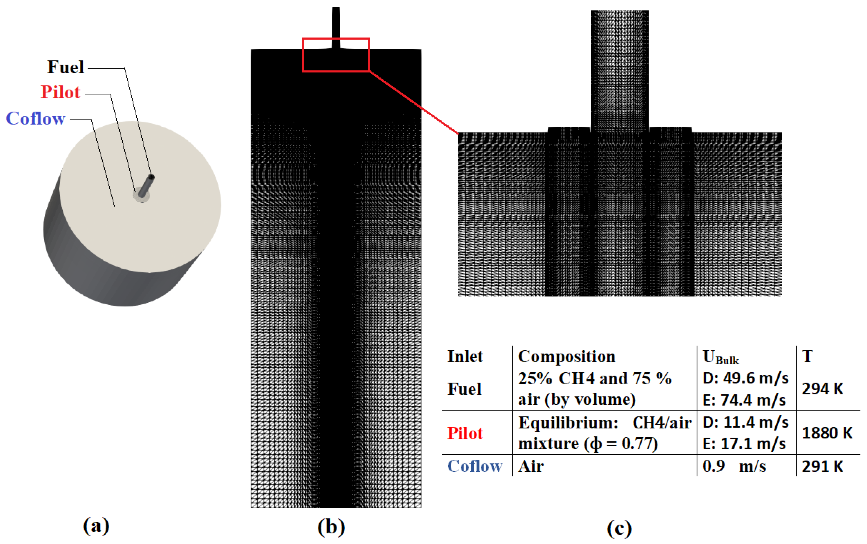
3. Case Studies: Flames D and E

3.1. Case Description

In this study, the LES hybrid ESF/FGM approach using eight stochastic fields is applied to evaluate the thermodynamic performance of Sandia flames D and E by means of an entropy generation analysis. The two flames share the same burner geometry, which features three inlet streams as shown in Figure 1. The fuel consists of a mixture of methane and air: 25% methane diluted in 75% air by volume. Figure 1a–c displays a sketch of the experimental and numerical configuration together with all the inflow/operating conditions.

Figure 1. Sandia flame burner. (a) Sketch of experimental configuration, (b) numerical grid and (c) inflow/operating conditions.

Figure 1. Sandia flame burner. (a) Sketch of experimental configuration, (b) numerical grid and (c) inflow/operating conditions.

A detailed description of the burner configuration, the flow field parameters and various scalar and velocity data obtained from measurements can be found in [52]. Simulations were carried out on a 3D structured hexahedral grid. Figure 1b shows some features of the used numerical grid with a total mesh size of 2.9 million cells. The grid is refined in the direction of the fuel jet, with a smallest cell of 1 × 10 ⁻¹¹ m⁻³.

To ensure the appropriate inflow conditions, synthetic turbulence and mapping methods are used. The procedure is as follows: Downstream of the fuel inlet, at the cross section 5.5d, the velocity was mapped onto the inlet fuel plane. However, synthetic turbulence had been applied to the pilot inlet. At the inlet and outlet boundary conditions, the total pressure was fixed to the atmospheric pressure.

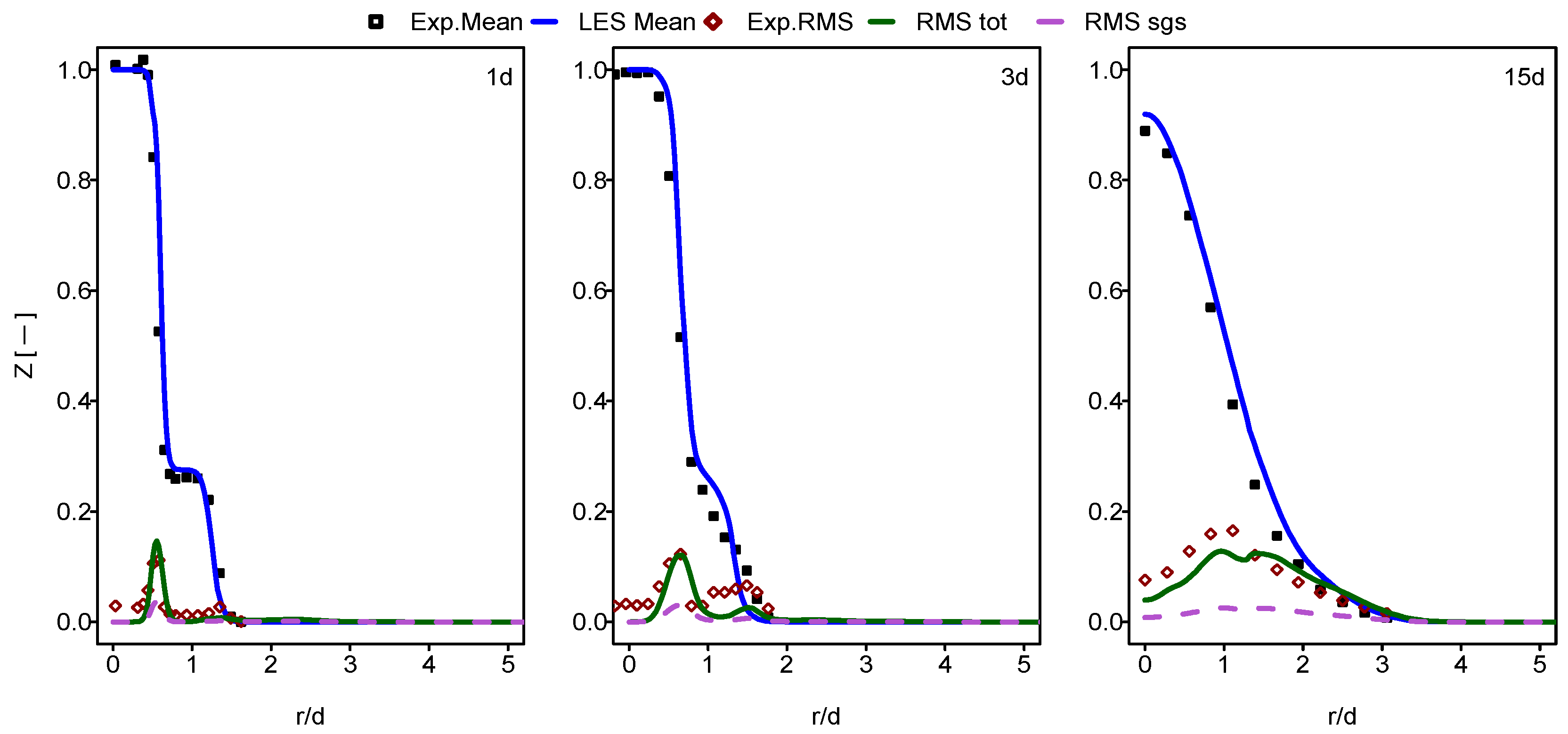
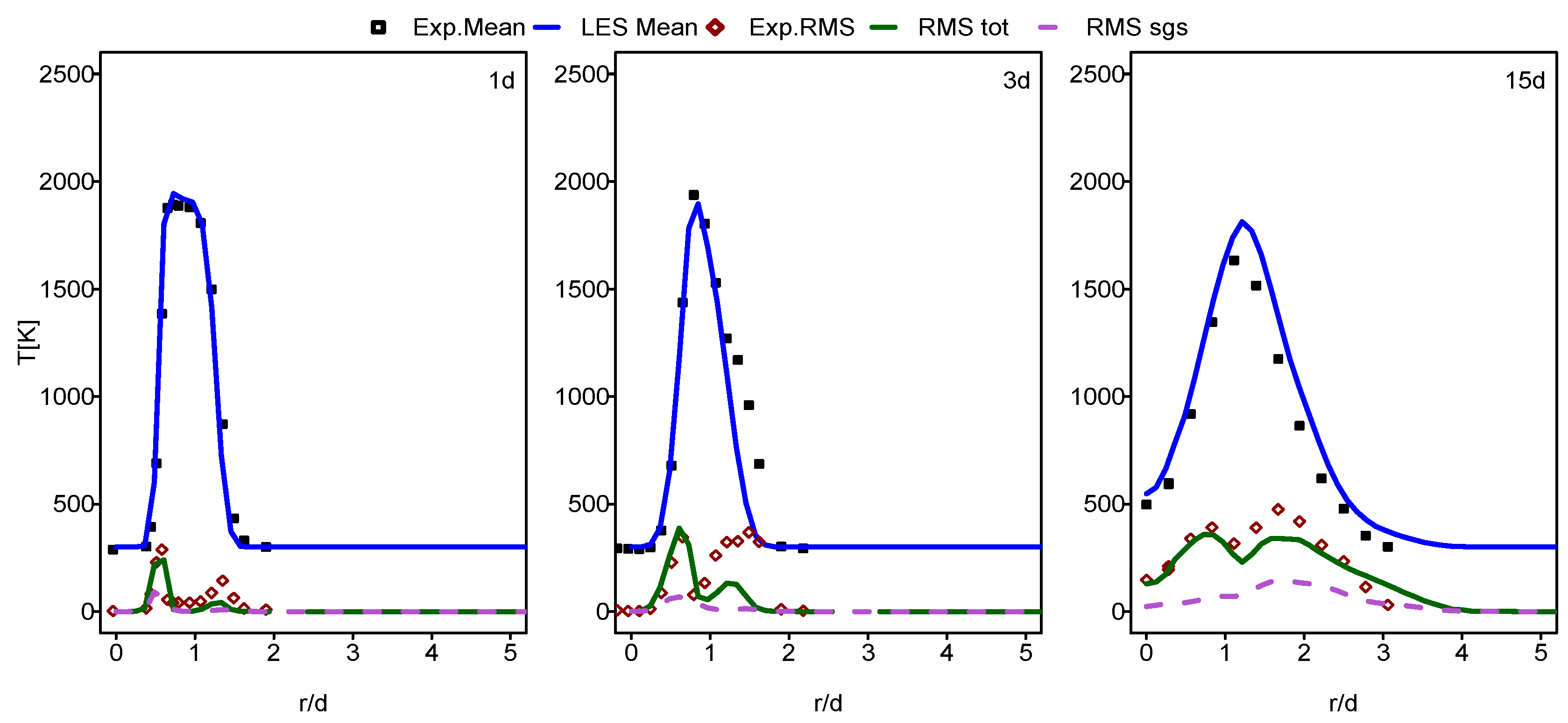
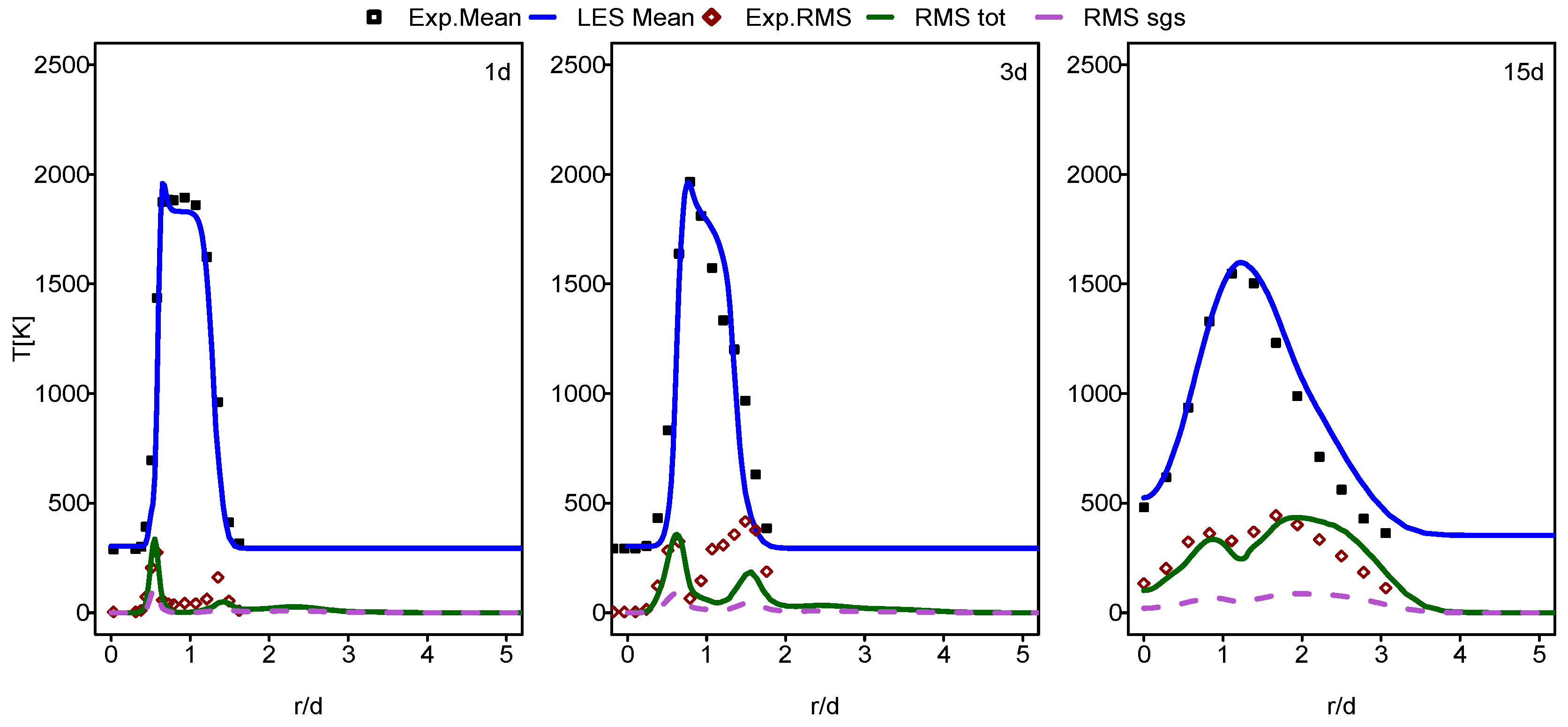
3.2. Case Validation

In this section, comparisons of the numerical results with experimental data for the scalar and flow field are provided. The results for the mean and RMS radial profiles of the mixture fraction and the temperature at three axial positions, 1d, 3d and 15d, are first compared to experimental data from [52]. Please note that for the RMS quantities, the time-averaged sub-grid contributions obtained from the ESF simulations are also displayed (shown as dashed lines). Figure 2 and Figure 3 show the mean and RMS mixture radial profiles for Sandia flames D and E, respectively. For both cases, a good agreement is achieved, except for some underestimations in regard to RMS values, especially at position 3d. Compared to the resolved part, the sub-grid contributions to the scalar fluctuations obtained by ESF methods look much smaller. Similar observations for the radial profiles of the temperature, depicted in Figure 4 and Figure 5 for Sandia flames D and E, respectively, can be made. It turns out that eight stochastic fields seem to be sufficient to ensure the higher accuracy of the simulation not only of Sandia flame D as reported in the literature [16,17,34], but also of flame E [16,17].

The instantaneous temperature and velocity contour plots are displayed in Figure 6. Increasing the velocity, especially for the fuel jet, from flame D to flame E leads to thickening of the flame. No extinction is found for flame D, which features typically diffused flame characteristics, whereas flame E exhibits extinction pockets which expand in few cells and re-ignite further downstream. This is also clearly shown in Figure 7, where the scatter plots of the experimental and numerical instantaneous temperature for both flames at the axial position 7.5d are provided. Here, one can clearly see the phenomenon of partial flameout for flame E and its absence for flame D.

4. Exergy Analysis: Results and Discussions

In this section, an exergetic analysis is performed for Sandia flames D and E. Thereby, the entropy generation contributions, due to the various sources of irreversibility intrinsically related to the processes and mechanisms interfering in these two turbulent flames, are quantified. Three different methods, namely the thermodynamics-based, the turbulence-based and the look-up-table-based approaches are used as described in Section 2.2.1, Section 2.2.2, Section 2.2.3. Recall that the viscous source term is calculated similarly in all approaches, and the source term due to the chemical reaction is closed and identical for all approaches. To estimate the minimal complexity the FGM table can accept to obtain convergent entropy source terms, especially for the heat and species mass diffusion contributions, a preliminary study has been carried out for the thermodynamic-based and the turbulence-based approaches. These two approaches have been tested within the RANS context using seven main species (CH₄, CO₂, CO, H₂O, O₂, H₂ and OH) and all species (53 species for this work). Both methods showed slight differences while using, respectively, 7 and 53 species for the heat source term. However, a great difference could be found for the species mass diffusion term when reducing the number of species. Therefore, a minimum of seven species are considered within the thermodynamic-based method for the heat source term Π_q, while all species are retained for the turbulence-based and the look-up-table-based methods.

Figure 8 presents the radial profiles of the volumetric entropy generation from heat transfer for the three approaches. The flame D and E results show comparable values. A higher value is observed for the thermodynamic approach, especially at the axial position 3d for flame E. Two local peaks in the inner (jet/pilot) shear layer near the nozzle (1d axial position) can be clearly seen for entropy production due to heat transfer. This is obvious because of the strong temperature gradients in these regions. Compared to flame D, the entropy generation rates due to heat transfer for flame E are higher. The presence of extinction pockets for this flame raises the temperature gradients, that, in turn, results in enhanced entropy generation.

The evaluation of entropy production from mass diffusion by the turbulence-based and look-up-table-based methods for flame D and E is illustrated in Figure 9. Both methods achieve consistent results. Similar peaks as for the entropy generation due to heat transfer are detected. However, local large values correspond here to large gradients in species concentrations, which are characterized by the mixture fraction gradient. As shown in the same plots, enhancing the species diffusion by increasing the inlet mass flow from flame D to E increases the entropy generation rate due to mass diffusion, which remains lower than that due to heat transfer for both flames.

In Figure 10, the entropy production due to chemical reaction is presented. The contribution of the chemical reaction is more or less comparable to the mass diffusion, but remains lower than that of the heat transfer term. It turns out that the contribution behavior in turbulent non-premixed flame is similar to that found in laminar cases [1]. However, the peaks for the entropy generation are found in the flame zone at the axial position near the nozzle (1d position), and an increase is observable at the downstream location (see 15d position). The chemical reaction significantly increases the concentration gradients, leading to the increase in entropy production. Higher values are found in flame E due to the increase in the inlet mass flow. The viscous dissipation contribution seems to be negligible compared to the other processes, as shown in Figure 11 for both flames. However, the increase in the fuel jet velocity in flame E increases the entropy generation rates. One peak is detected in the jet fuel zone near the nozzle inlet for both flames, where a strong shearing process occurs.

A general conclusion from Figure 8, Figure 9, Figure 10 and Figure 11 is that all entropy generation sources show larger prevalence in the radial direction downstream of the burner (axial position 15d) where the turbulent jet develops. The entropy generation rates for Sandia flame D are found to be consistent and comparable with those reported in the literature [12]. However, the novel approaches are 20 and 1.5× less for the look-up-table-based and the turbulence-based approaches, respectively, than the thermodynamic-based method in terms of computational cost.

In Figure 12, Figure 13, Figure 14 and Figure 15, the instantaneous contour plots of the entropy generation associated with heat transfer, mass diffusion, viscous dissipation and the chemical reaction as well as the contribution ratio of each process for flames D and E, respectively, are displayed using the inexpensive look-up-table-based method. For both cases, the first three entropy production terms show their higher values in the jet zone and near the nozzle exit. However, the entropy generation due to the chemical reaction is mainly located in the flame zone and downstream the burner. The heat transfer and the chemical reaction feature the major process contributions to the total entropy generation. However, near the nozzle exit (at 1d position), the contribution of the mass diffusion exceeds the chemical reaction contribution in accordance with Figure 6c,d and this is intensified in flame E compared to flame D, as the jet Re number is increased.

5. Conclusions

The LES hybrid ESF/FGM approach was used to investigate the irreversibilities that evolve in Sandia flames D and E. The predictive capability of this approach is higher at a lower cost by using only eight stochastic fields. First, a good prediction of different scalar and flow field quantities is reported. Flame D shows no partial flameout contrary to the flame E, which exhibits some extinction pockets. Regarding the second law analysis, the main novelty of this paper consists of comparing the classical-thermodynamics-based approach with two novel methods, the turbulence-based and the look-up-table-based approaches suggested for the computation of entropy generation in combustion systems without solving the whole entropy transport equation. Using flame D as a reference, for which some results with the thermodynamic-based approach are available in the literature [12], the following conclusions can be drawn:

• Good agreements are observed between the results obtained by using the two novel approaches suggested in the present paper and those reported in the literature for the mean entropy production rates and distribution in the case of flame D.
• The effect of the mass flow rate along with the Re number on the entropy production rates has been pointed out from the analysis performed for flame E in comparison to the reference, flame D. In particular:
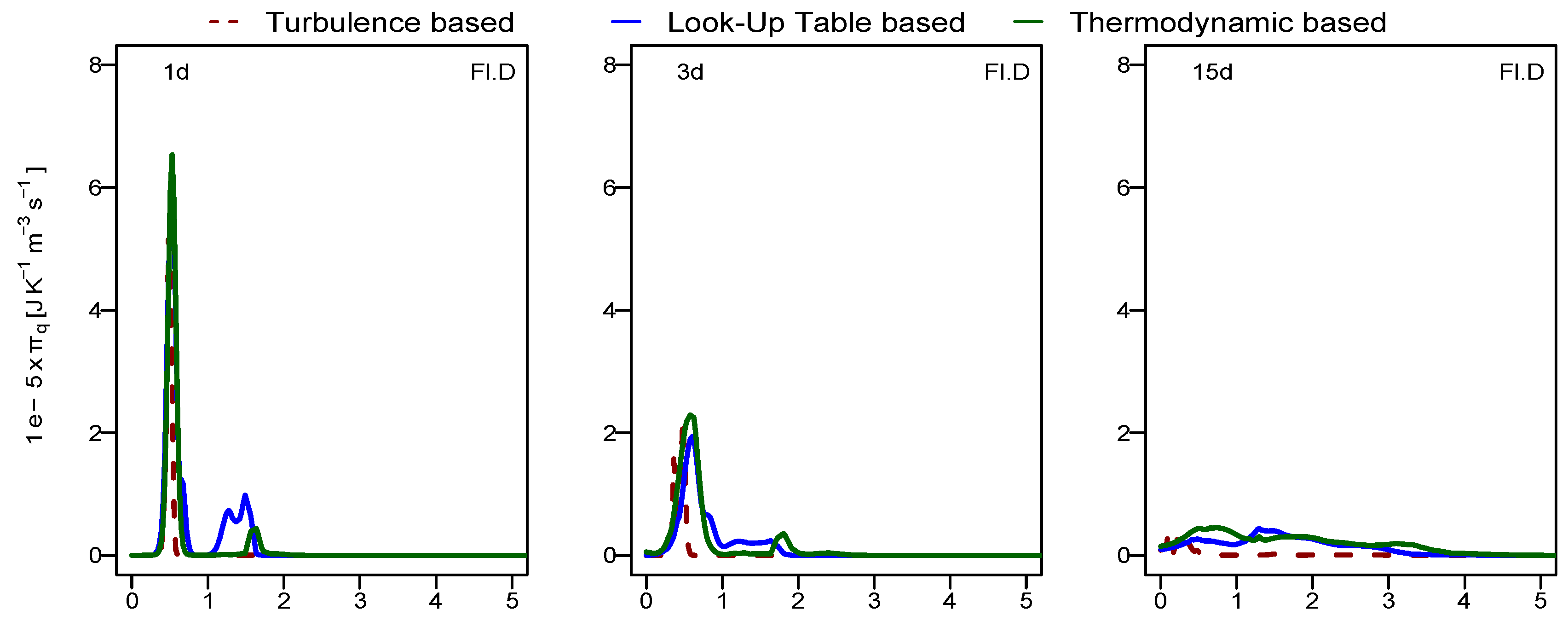
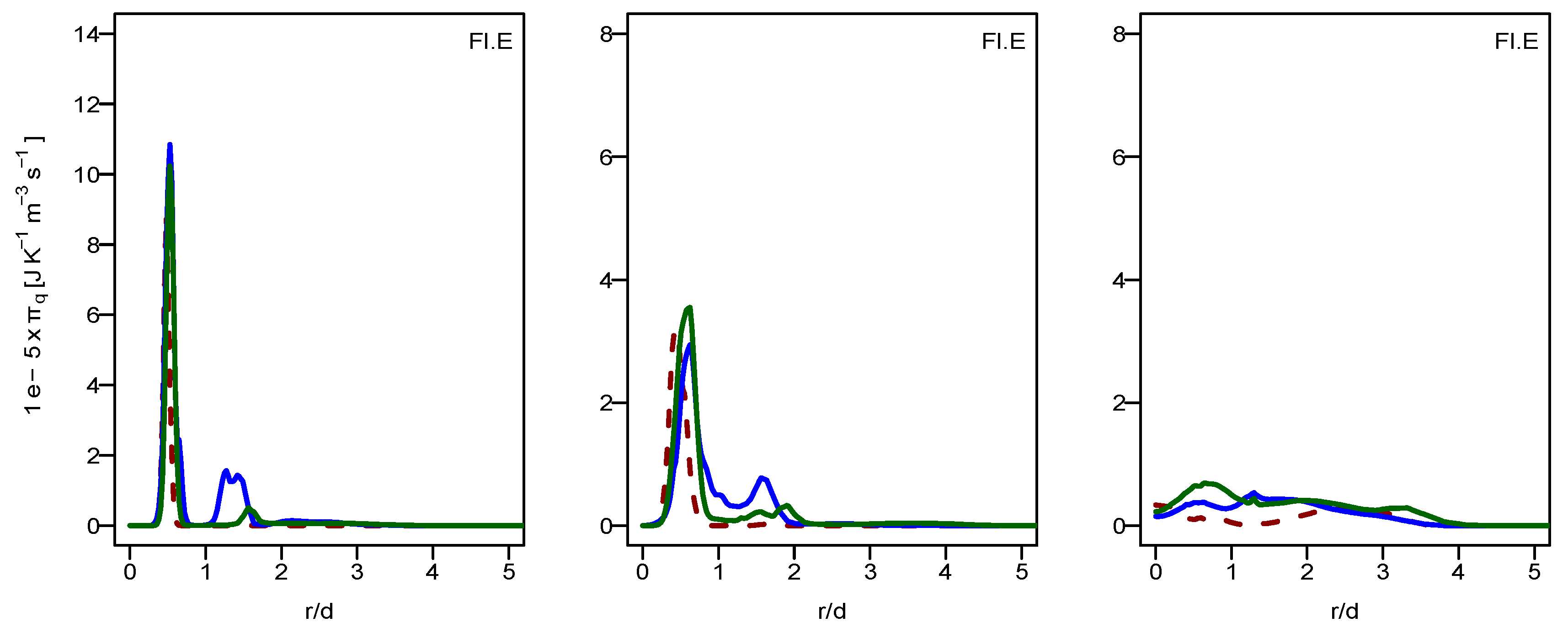
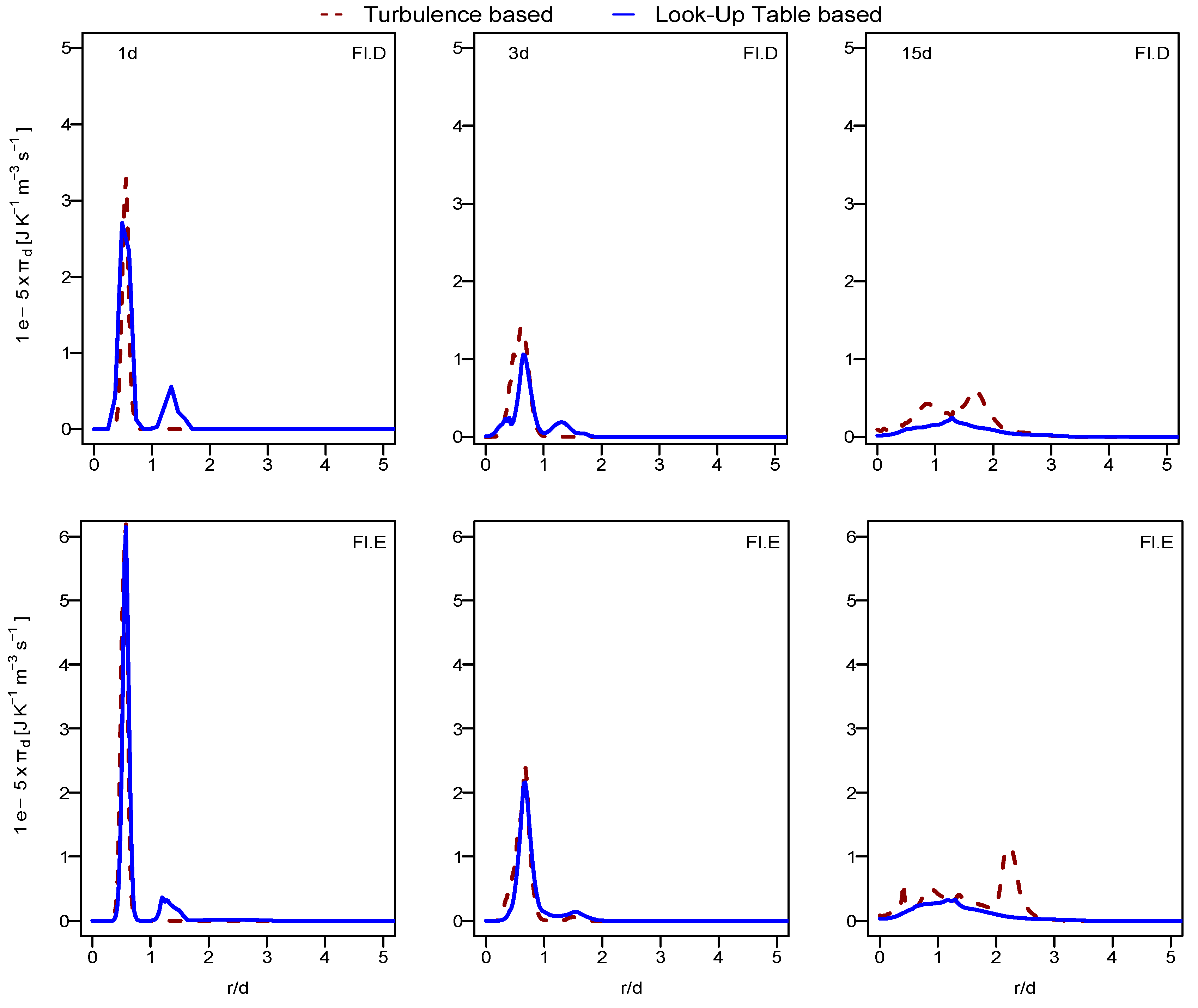
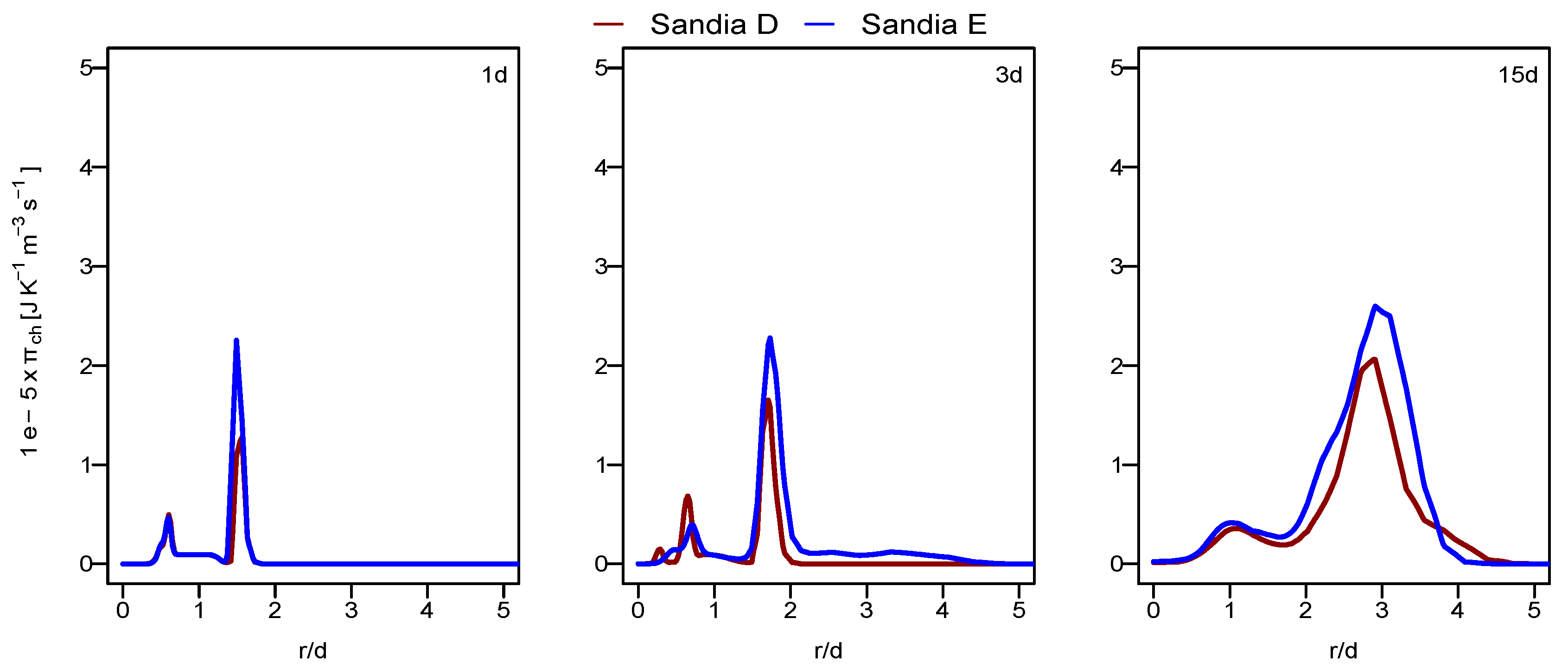
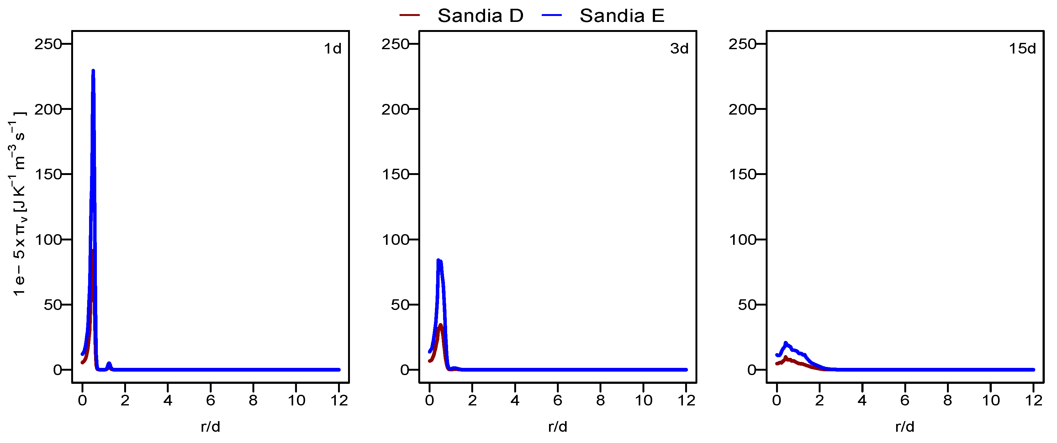
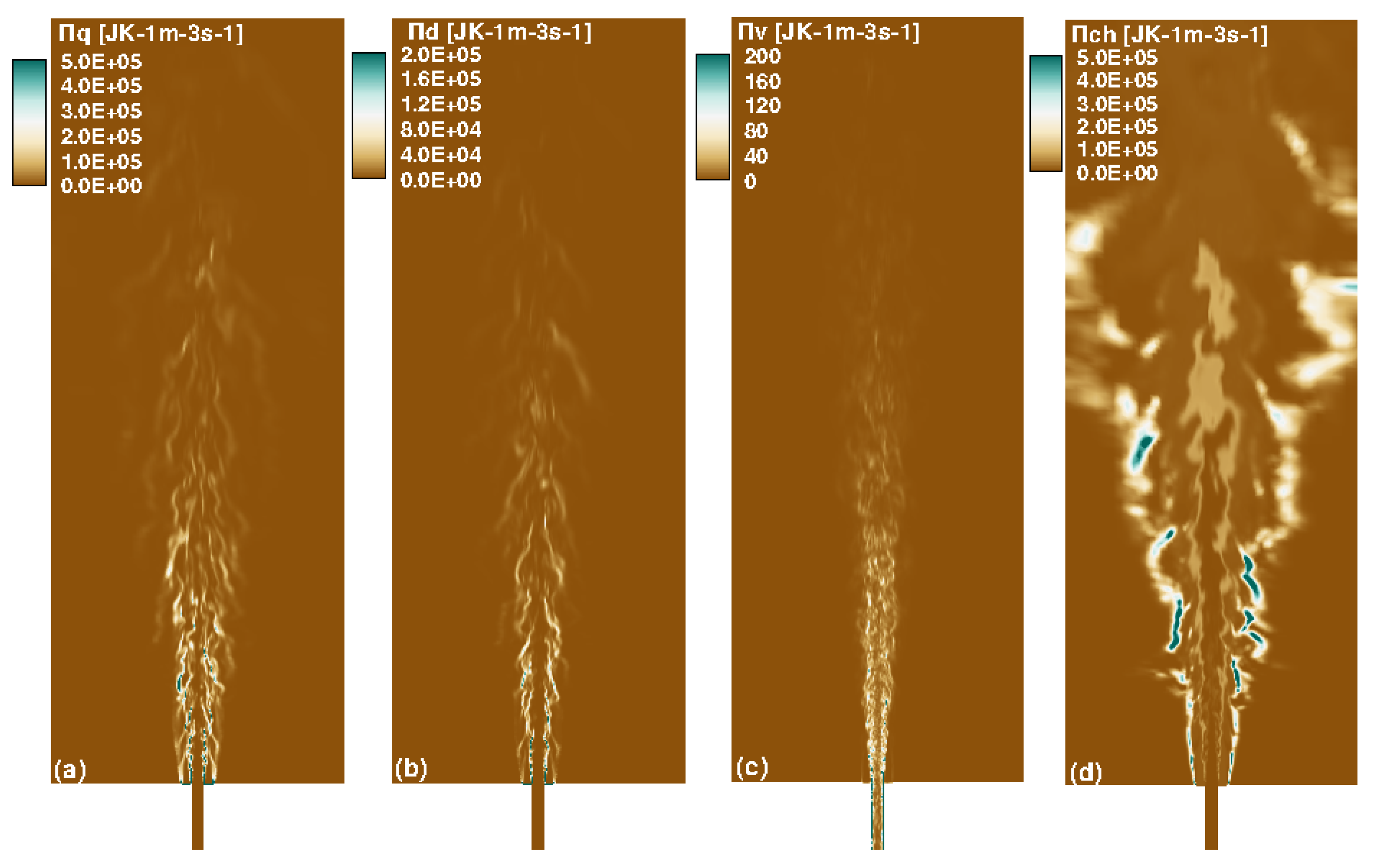
  • A peak of entropy generation is detected at the axial position close to the fuel nozzle for all the entropy generation terms.
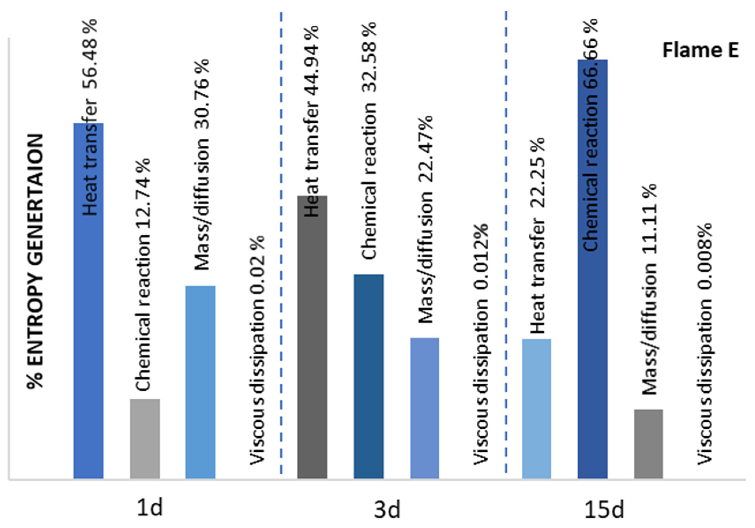
  • The radial profile of the entropy generation highlights the decrease in entropy downstream; the peaks vanish, except for entropy production due to the chemical reaction, in which a new peak is observed.
• The entropy generation contributions due to the heat transfer and chemical reaction processes dominate those due to diffusion and viscous dissipation.
• The entropy generation rates augment from flame D to flame E. This is explained by the increase in temperature, velocity and concentration gradients induced by a high mass flow rate associated with flame E.
• The computational cost appears to be less once the entropy generation analysis is performed by using the LES hybrid ESF/FGM approach together with the look-up-table-based or the turbulence-based approach.

In this paper, the LES hybrid ESF/FGM approach seems to be efficient for computing Sandia flame D and E. It is of paramount interest to complete this study with a parametric study to optimize the thermodynamic efficiency of these combustion systems using the LES hybrid ESF/FGM approach. Potential is left for future work together with the extension of this analysis to Sandia flame F.

References

1. Nishida, K.; Takagi, T.; Kinoshita, S. Analysis of entropy generation and exergy loss during combustion. Proc. Comb. Inst. 2002, 29, 869–874. [Google Scholar] [CrossRef]
2. Keenan, J.G. Availability and irreversibility in thermodynamics. Brit. J. Appl. Phys. 1951, 2, 183–192. [Google Scholar] [CrossRef]
3. Bejan, A. Fundamentals of exergy analysis, entropy generation minimization, and the generation of flow architecture. Int. J. Energy Res. 2002, 26, 545–565. [Google Scholar] [CrossRef]
4. Som, S.K.; Datta, A. Thermodynamic irreversibilities and exergy balance in combustion processes. Prog. Energ. Combust. 2008, 34, 351–376. [Google Scholar] [CrossRef]
5. Sciacovelli, A.; Verda, V.; Sciubba, E. Entropy generation analysis as a design tool—A review. Renew. Sust. Energ. Rev. 2015, 43, 1167–1181. [Google Scholar] [CrossRef]
6. Hirschefelder, J.O.; Curtiss, C.F.; Bird, R.B. Molecular Theory of Gases and Liquids; Wiley: Hoboken, NJ, USA, 1954. [Google Scholar]
7. Ries, F.; Li, Y.; Klingenberg, D.; Nishad, K.; Janicka, J.; Sadiki, A. Near-wall thermal processes in an inclined impinging jet: Analysis of heat transport and entropy generation mechanisms. Energies 2018, 11, 1354. [Google Scholar] [CrossRef] [Green Version]
8. Ries, F.; Li, Y.; Nishad, K.; Janicka, J.; Sadiki, A. Entropy generation analysis and thermodynamic optimization of jet impinge-ment cooling using large eddy simulation. Entropy 2019, 19, 129. [Google Scholar] [CrossRef] [Green Version]
9. Ziefuss, M.; Karimi, N.; Ries, F.; Sadiki, A.; Mehdizadeh, A. Entropy generation assessment for wall-bounded turbulent shear flows based on Reynolds analogy assumptions. Entropy 2019, 21, 1157. [Google Scholar] [CrossRef] [Green Version]
10. Ries, F.; Kütemeier, D.; Li, Y.; Nishad, K.; Sadiki, A. Effect chain analysis of supercritical fuel disintegration processes using an Les-based entropy generation analysis. Combust. Sci. Technol. 2020, 192, 2171–2188. [Google Scholar] [CrossRef]
11. Safari, M.; Sheikhi, M.R.H.; Janbozorgi, M.; Metghalchi, H.; Sheikhi, R.H. Entropy transport equation in large eddy simulation for exergy analysis of turbulent combustion systems. Entropy 2010, 12, 434. [Google Scholar] [CrossRef]
12. Safari, M.; Hadi, F.; Sheikhi, M.R.H. Progress in the Prediction of entropy generation in turbulent reacting flows using large eddy simulation. Entropy 2014, 16, 5159–5177. [Google Scholar] [CrossRef] [Green Version]
13. Pope, S. PDF methods for turbulent reactive flows. Prog. Energy Combust. Sci. 1985, 11, 119–192. [Google Scholar] [CrossRef]
14. Pope, S.B. A monte carlo method for the PDF equations of turbulent reactive flow. Combust. Sci. Technol. 1981, 25, 159–174. [Google Scholar] [CrossRef]
15. Prasad, V.N. Large Eddy Simulation of Partially Premixed Turbulent Combustion. Ph.D. Thesis, Imperial College London, University of London, London, UK, 2011. [Google Scholar]
16. Jones, W.; Prasad, V. Large eddy simulation of the Sandia flame series (D–F) using the Eulerian stochastic field method. Combust. Flame 2010, 157, 1621–1636. [Google Scholar] [CrossRef]
17. Yifan, D.U.A.N.; Zhixun, X.I.A.; Likun, M.A.; Zhenbing, L.U.O.; Huang, X.; Xiong, D.E.N.G. LES of the Sandia flame series D-F using the Eulerian stochastic field method coupled with tabulated chemistry. Chin. J. Aeronaut. 2020, 33, 116–133. [Google Scholar]
18. Jejurkar, S.Y.; Mishra, D.P. Numerical analysis of entropy generation in a annular micro combustor using multistep kinetics. Appl. Therm. Eng. 2013, 52, 394–401. [Google Scholar] [CrossRef]
19. Wenming, Y.; Dongyue, J.; Kenny, C.K.Y.; Dan, Z.; Jianfeng, P. Combustion process and entropy generation in a novel micro combustor with a block insert. J. Chem. Eng. 2015, 274, 231–237. [Google Scholar] [CrossRef]
20. Morsli, S.; Sabeur, A.; El Ganaoui, M.; Ramenah, H. Computational simulation of entropy generation in a combustion chamber using a single burner. Entropy 2018, 20, 922. [Google Scholar] [CrossRef] [Green Version]
21. Safer, K.; Ouadha, A.; Tabet, F. Entropy generation in turbulent syngas counter-flow diffusion flames. Int. J. Hydrogen Energy 2017, 42, 29532–29544. [Google Scholar] [CrossRef]
22. Mohammadi, I.; Ajam, H. A theoretical study of entropy generation of the combustion phenomenon in the porous media burner. Energy 2019, 188, 116004. [Google Scholar] [CrossRef]
23. Zuo, W.; Zhang, Y.; Li, J.; Li, Q.; He, Z. A modified micro reactor fueled with hydrogen for reducing entropy generation. Int. J. Hydrogen Energy 2019, 44, 27984–27994. [Google Scholar] [CrossRef]
24. Ni, S.; Zhao, D.; Sun, Y.; Jiaqiang, E. Numerical and entropy studies of hydrogen-fuelled micro-combustors with different geometric shaped ribs. Int. J. Hydrogen Energy 2019, 44, 7692–7705. [Google Scholar] [CrossRef]
25. Ansari, M.; Amani, E. Micro-combustor performance enhancement using a novel combined baffle-bluff configuration. Chem. Eng. Sci. 2018, 175, 243–256. [Google Scholar] [CrossRef]
26. Wang, W.; Zuo, Z.; Liu, J.; Yang, W. Entropy generation analysis of fuel premixed CH4 /H2 /air flames using multistep kinetics. Int. J. Hydrogen Energy 2016, 41, 20744–20752. [Google Scholar] [CrossRef]
27. Salimath, P.S.; Ertesvåg, I.S. Local entropy generation and entropy fluxes of a transient flame during head-on quenching towards solid and hydrogen-permeable porous walls. Int. J. Hydrogen Energy 2021, 46, 26616–26630. [Google Scholar] [CrossRef]
28. Bykov, V.; Maas, U. The extension of the ILDM concept to reaction–diffusion manifolds. Combust. Theory Model. 2007, 11, 839–862. [Google Scholar] [CrossRef]
29. Pierce, C.D.; Moin, P. Progress-variable approach for large-eddy simulation of non-premixed turbulent combustion. J. Fluid Mech. 2004, 504, 73–97. [Google Scholar] [CrossRef]
30. Fiorina, B.; Veynante, D.; Candel, S. Modeling combustion chemistry in large eddy simulation of turbulent flames. Flow Turbul. Combust. 2014, 94, 3–42. [Google Scholar] [CrossRef]
31. Vicquel, R. Tabulated Chemistry for Turbulent Combustion Modeling and Simulation. Ph.D. Thesis, Laboratoire d’Énergétique Moléculaire et Macroscopique, Combustion (EM2C) du CNRS et de l’ECP, Ecole Centrale Paris, Paris, France, June 2010. [Google Scholar]
32. van Oijen, J.; Donini, A.; Bastiaans, R.; Boonkkamp, J.T.T.; de Goey, L. State-of-the-art in premixed combustion modeling using flamelet generated manifolds. Prog. Energy Combust. Sci. 2016, 57, 30–74. [Google Scholar] [CrossRef] [Green Version]
33. Bilger, R.W.; Stårner, S.H.; Kee, R.J. On reduced mechanisms for methane-air combustion in non-premixed flames. Combust. Flame 1990, 80, 135–149. [Google Scholar] [CrossRef]
34. Mahmoud, R.; Jangi, M.; Ries, F.; Fiorina, B.; Janicka, J.; Sadiki, A. Combustion characteristics of a non-premixed oxy-flame applying a hybrid filtered eulerian stochastic field/flamelet progress variable approach. Appl. Sci. 2019, 9, 1320. [Google Scholar] [CrossRef] [Green Version]
35. Goodwin, D.; Moffat, H.K. Cantera. Available online: http://code.google.com/p/cantera/ (accessed on 28 June 2021).
36. Nicoud, F.; Toda, H.B.; Cabrit, O.; Bose, S.; Lee, J. Using singular values to build a subgrid-scale model for large eddy simula-tions. Phys. Fluids 2011, 23, 085106. [Google Scholar] [CrossRef] [Green Version]
37. Valiño, L. A field monte carlo formulation for calculating the probability density function of a single scalar in a turbulent flow. Flow Turbul. Combust. 1998, 60, 157–172. [Google Scholar] [CrossRef]
38. Dopazo, C.; O’Brien, E.E. Functional formulation of non-isothermal turbulent reactive flows. Phys. Fluids 1974, 17, 1968–1975. [Google Scholar] [CrossRef] [Green Version]
39. Dressler, L.; Filho, F.L.S.; Ries, F.; Nicolai, H.; Janicka, J.; Sadiki, A. Numerical prediction of turbulent spray flame characteristics using the filtered eulerian stochastic field approach coupled to tabulated chemistry. Fluids 2021, 6, 50. [Google Scholar] [CrossRef]
40. Jones, W.P.; Navarro-Martinez, S.; Röhl, O. Large eddy simulation of hydrogen auto-ignition with a probability density function method. Proc. Combust. Inst. 2007, 31, 1765–1771. [Google Scholar] [CrossRef]
41. Avdi´c, A.; Kuenne, G.; di Mare, F.; Janicka, J. LES combustion modeling using the Eulerian stochastic field method coupled with tabulated chemistry. Combust. Flame 2017, 175, 201–219. [Google Scholar] [CrossRef]
42. Frost, V.A. Model of a turbulent, diffusion-controlled flame jet. Fluid Mech. Soviet Res. 1975, 4, 124–133. [Google Scholar]
43. O’Brien, E.E. The probability density function (pdf) approach to reacting turbulent flows. In Turbulent Reacting Flows; Springer: Berlin/Heidelberg, Germany, 1980; pp. 185–218. [Google Scholar] [CrossRef]
44. Villermaux, J.; Falk, L. A generalized mixing model for initial contacting of reactive fluids. Chem. Eng. Sci. 1994, 49, 5127–5140. [Google Scholar] [CrossRef]
45. Kloeden, P.E.; Platen, E. Numerical Solution of Stochastic Differential Equations; Springer Science & Business Media: New York, NY, USA, 1992. [Google Scholar]
46. Picciani, M.A. Investigation of Numerical Resolution Requirements of the Eulerian Stochastic Fields and the Thickened Sto-chastic Field Approach. Ph.D. Thesis, University of Southampton, Southampton, UK, 2018. [Google Scholar]
47. Muradoglu, M.; Jenny, P.; Pope, S.B.; Caughey, D.A. A consistent hybrid finite-volume/particle method for the PDF equations of turbulent reactive flows. J. Comput. Phys. 1999, 154, 342–371. [Google Scholar] [CrossRef] [Green Version]
48. Ries, F.; Obando, P.; Shevchuck, I.; Janicka, J.; Sadiki, A. Numerical analysis of turbulent flow dynamics and heat transport in a round jet at supercritical conditions. Int. J. Heat Fluid Flow 2017, 66, 172–184. [Google Scholar]
49. Issa, R. Solution of the implicitly discretized fluid flow equations by operator-splitting. J. Comput. Phys. 1986, 62, 40–65. [Google Scholar] [CrossRef]
50. Patankar, S.; Spalding, D. A calculation procedure for heat, mass and momentum transfer in three-dimensional parabolic flows. In Numerical Prediction of Flow, Heat Transfer, Turbulence and Combustion; Patankar, S.V., Pollard, A., Singhal, A.K., Eds.; Pergamon: Oxford, UK, 1983; pp. 54–73. [Google Scholar] [CrossRef]
51. Garmory, A. Micro-mixing Effects in Atmospheric Reacting Flows. Ph.D. Thesis, University of Cambridge, Cambridge, UK, 2008. [Google Scholar]
52. TNF Workshop. Available online: http://www.ca.sandia.gov/TNF (accessed on 28 June 2021).
53. Safari, M.; Sheikhi, M.R.H. Large eddy simulation for prediction of entropy generation in a non-premixed turbulent jet flame. J. Energy Resour. Technol. 2014, 136, 022002. [Google Scholar] [CrossRef]
54. Sheikhi, M.R.H.; Safari, M.; Metghalchi, H. Large Eddy simulation for local entropy generation analysis of turbulent flows. J. Energy Resour. Technol. 2012, 134, 041603. [Google Scholar] [CrossRef]
55. Sheikhi, M.R.H.; Givi, P.; Pope, S.B. Frequency-velocity-scalar filtered mass density function for large eddy simulation of turbulent flows. Phys. Fluids 2009, 21, 075102. [Google Scholar] [CrossRef] [Green Version]
56. Sheikhi, M.R.H.; Givi, P.; Pope, S.B. Velocity-scalar filtered mass density function for large eddy simulation of turbulent reacting flows. Phys. Fluids 2007, 19, 95106. [Google Scholar] [CrossRef]
57. Sheikhi, M.R.H.; Drozda, T.G.; Givi, P.; Pope, S.B. Velocity-scalar filtered density function for large eddy simulation of turbulent flows. Phys. Fluids 2003, 15, 2321. [Google Scholar] [CrossRef] [Green Version]
58. Lilly, D. The representation of small-scale turbulence in numerical simulation experiments. IBM Form 1967, 281, 95–210. [Google Scholar] [CrossRef]
59. Schmidt, H.; Schumann, U. Coherent structure of the convective boundary layer derived from large-eddy simulations. J. Fluid Mech. 1989, 200, 511–562. [Google Scholar] [CrossRef] [Green Version]
60. Corrsin, S. On the spectrum of isotropic temperature fluctuations in an isotropic turbulence. J. Appl. Phys. 1951, 22, 469–473. [Google Scholar] [CrossRef]
Figure 2. Mixture fraction at different axial positions: comparison for flame D. The dashed line represents the unresolved contribution to the RMS.
Energies 14 06315 g002
Figure 3. Mixture fraction at different axial positions: comparison for flame E.
Energies 14 06315 g003
Figure 4. Temperature at different axial positions: comparison for flame D.
Energies 14 06315 g004
Figure 5. Temperature at different axial positions: comparison for flame E.
Energies 14 06315 g005
Figure 6. Contour plots of instantaneous axial velocity: (a) Sandia D, (b) Sandia E and instantaneous temperature: (c) Sandia D, (d) Sandia E.
Energies 14 06315 g006
Figure 7. Instantaneous scatter plots of temperature versus mixture fraction for flames D and E at axial position 7.5d.
Energies 14 06315 g007
Figure 8. Radial profile of the volumetric entropy from heat transfer: comparison of the three approaches (thermodynamics-based, the turbulence-based and the look-up-table-based approach) at various axial positions for flame D (top) and flame E (bottom).
Energies 14 06315 g008aEnergies 14 06315 g008b
Figure 9. Radial profile of the volumetric entropy from mass diffusion of species: comparison of results using the turbulence-based and the look-up-table-based approaches at various axial positions for flame D (top) and flame E (bottom).
Energies 14 06315 g009
Figure 10. Radial profile of the volumetric entropy caused by the chemical reaction at various axial positions for flame D (red) and flame E (blue).
Energies 14 06315 g010
Figure 11. Radial profile of the volumetric entropy caused by viscous dissipation at various axial positions for flame D (red) and flame E (blue).
Energies 14 06315 g011
Figure 12. Contour plots of instantaneous volumetric entropy using the look-up-table-based method for flame D caused by: (a) heat transfer, (b) mass diffusion, (c) viscous dissipation and (d) the chemical reaction.
Energies 14 06315 g012
Figure 13. Entropy generation ratio of each process at different axial positions using the look-up-table-based method for Sandia flame D.
Energies 14 06315 g013
Figure 14. Contour plots of instantaneous volumetric entropy using the look-up-table-based method for flame E caused by: (a) heat transfer, (b) mass diffusion, (c) viscous dissipation and (d) the chemical reaction.
Energies 14 06315 g014
Figure 15. Entropy generation ratio of each process at different axial positions using the look-up-table-based method for Sandia flame E.
Energies 14 06315 g015
Publisher’s Note: MDPI stays neutral with regard to jurisdictional claims in published maps and institutional affiliations.