Energy Consumption-Based Maintenance Policy Optimization

Abstract

The optimal predictive, preventive, corrective and opportunistic maintenance policies play an important role in the success of sustainable maintenance operations. This study discusses a new energy efficiency-related maintenance policy optimization method, which is based on failure data and status information from both the physical system and the digital twin-based discrete event simulation. The study presents the functional model, the mathematical model and the solution algorithm. The maintenance optimization method proposed in this paper is made up of four main phases: computation of energy consumption based on the levelized cost of energy, computation of GHG emission, computation of value determination equations and application of the Howard’s policy iteration techniques. The approach was tested with a scenario analysis, where different electricity generation sources were taken into consideration. The computational results validated the optimization method and show that optimized maintenance policies can lead to an average of 38% cost reduction regarding energy consumption related costs. Practical implications of the proposed model and method regard the possibility of finding optimal maintenance policies that can affect the energy consumption and emissions from the operation and maintenance of manufacturing systems.

1. Introduction

Today, significant changes are taking place in production and service systems as the impact of the Fourth Industrial Revolution is felt, resulting not only in significant quantitative but also qualitative changes. These changes affect not only the production processes, but also other important activities related to their operation, such as procurement, distribution and maintenance. In the case of complex systems, the implementation of design tasks requires an integrated approach [1], through which both investment and operating costs can be reduced while a sustainable system can be implemented. As statistical surveys show, the top causes for maintenance are the following: 34% aging resources, 20% mechanical failure of equipment, 11% human and operational error, 9% lack of time for maintenance, and 8% bad design of technical and logistics resources [2]. These are influencing the energy efficiency and energy consumption of manufacturing systems; therefore, these complex causes require complex maintenance policy. The application of maintenance policies in digital contexts is a new trend in the Industry 4.0 era. Digital twin-based simulation makes it possible to optimize the operation and maintenance of manufacturing systems, because the impact of maintenance policies can be validated through discrete event simulation [3]. The digital twin methodology is used in many fields of manufacturing, construction and oil industry, and new research shows that this technology is applicable in the field of risk control and prevention [4]. Energy efficiency plays an important role in the manufacturing processes, where smart production systems apply preventive maintenance and restoration to prevent out-of-control states [5]. Maintenance policies can be applied in complex supply chain solutions with maintenance and warranty policy [6]. A wide range of studies focus on the maintenance policies of imperfect production systems [7], but only a few of them analyze the impact of these policies on energy efficiency and emission reduction.

A suitable maintenance policy has a great impact on the reduction of energy use, because a well-chosen preventive or corrective maintenance strategy can keep assets in the best condition, which leads to energy efficient operation; digital and automated work orders regarding maintenance can support the standardization of maintenance operation; identification of the real problems in the manufacturing system can identify the reasons for increased excessive energy consumption. Within the frame of this paper the proposed maintenance optimization methodology links maintenance optimization to the reduction of energy consumption. This paper studies the impact of maintenance policy optimization on energy consumption and GHG emission, while discounted profit is also taken into consideration. As the literature review section will show, the majority of the articles in the field of maintenance policy optimization are focusing on the optimization in a conventional manufacturing environment and only a few of them describes the maintenance policy and strategy optimization using digital-twin-based discrete event simulation regarding energy consumption and GHG emission depending on the electricity generation sources. The application of suitable design and control methods can increase the efficiency, availability and sustainability. Figure 1 summarizes the background of this research focusing on the linkage of energy and maintenance policy optimization.

This paper is organized as follows. Section 2 presents a systematic literature review, which summarizes the research background of manufacturing policy optimization from a descriptive and content analysis point of view. Section 3 describes the model framework of maintenance policy optimization including the functional model, the mathematical model and a Howard’s policy iteration-based optimization. The model is focusing on the energy consumption related costs based on a levelized cost of electricity. The model also takes into consideration GHG emissions depending on their source of generation. Section 4 demonstrates the scenario analysis, which validates the model and the optimization algorithm. Conclusions, future research directions and managerial impacts are discussed in Section 5.

2. Literature Review

Within the frame of this short systematic literature review the following questions are answered regarding maintenance policy optimization [8]: What is the current state of knowledge on maintenance related research? How is maintenance policy optimization analyzed and supported in previous works? What methods and parameters are used? What factors influence the results of maintenance policy optimization? Who first did it or published it? What are the main research gaps and what are the limitations of existing research results?

2.1. Systematic Literature Review Methodology

The used systematic literature review process can be divided into two main parts. The first part includes a descriptive analysis showing the tendencies of research topics in the field of maintenance policy optimization, while the second part focuses on the content analysis of the available research results. The used methodology of systematic literature review includes the following aspects: (a) definition of research questions; (b) search process in Science Direct; (c) inclusion and exclusion process; (d) descriptive analyses of chosen articles; (e) content analysis and (f) identification of scientific gaps, bottlenecks, and limitations (see Figure 2).

Firstly, the relevant terms were defined. The following keywords were used to search in the Science Direct database: “maintenance” AND “policy” AND “optimisation”. Initially, 42 articles were identified. This list was reduced to 33 articles by selecting journal articles only. The search was conducted in July 2021; therefore, new articles may have been published since then.

2.2. Descriptive Analysis

The journal articles focusing on maintenance policy optimization can be classified based on the subject area defined in Science Direct. Figure 3 shows the results of the classification of 33 articles considering 8 subject areas. This classification shows the majority of engineering, mathematics, computer sciences, and decision making.

The optimization of maintenance strategies and maintenance policies, especially in the field of manufacturing, production and transportation, has been intensively researched in the past 15 years, but there are some early research results from the 70s and 80s. One of the first articles in this field was published in 1978 in the field of optimization of stochastic maintenance policies [9] and within the frame of this article the author summarizes the main types of maintenance policies focusing on both deterministic and stochastic environment from a cost optimization point of view.

2.3. Content Analysis

As the descriptive analysis part of the systematic literature review shows, there is a wide range of articles regarding maintenance policy optimization. The literature sources focus on both modelling and optimization problems of maintenance strategies and validate the proposed policy optimization methods with different types of scenarios. Within the frame of this chapter, the most important results of maintenance policy optimization research are summarized. The results of the content analysis are summarized in Figure 4.

The time-dependent and average unavailability has a great impact on the performance of standby units, therefore several basic cost rate equation-based general formalisms were developed to support the selection process for optimal test and maintenance periods, where risk constraints were also taken into consideration [10]. The Markov Decision Process (MDP) is a general method which can be applied in the case of a wide range of maintenance strategy optimization problems. MDP-based modelling makes it possible to describe and optimize stochastic dynamic decision-making processes of condition-based maintenance. This modelling method means the integration of failure rate curves and non-convex mixed integer non-linear programming (MINLP), where the complexity of the model led to computational problems [11]. The integration of statistical process control and preventive maintenance plays an important role in the reliability and quality of production processes, because cost savings can be achieved by applying the optimized policy of preventive and corrective maintenance. In this approach the deterioration of production and logistics resources can be described as a discrete-time Markov chain model [12]. The inspection and maintenance policies in manufacturing systems generally focus on the reliability, availability and life-cycle cost of the production and material handling resources. The Markov-Decision-Process-based policy optimization can be integrated with Value of Information (VoI) methodology. This VoI-based MDB approach is used to find the ideal aperiodic sequential inspection and condition-based maintenance policy, where the decision-making process and its results depends on the value of information [13]. The optimization of inspection and maintenance strategies and policies is unavoidable in the case of preparedness systems, where failures can be detected only by inspections. A wide range of inspection and maintenance strategies can be taken into consideration and it is also a suitable way to mix various approaches and policies. The solution algorithm of preparedness systems can be based on both MDP and dynamic programming [9]. The efficiency of maintenance policies has a great impact on the quality of processes and products, therefore it is important to find the correct correlation between maintenance strategy and quality of products and processes. The relationship between maintenance and quality is influenced by a wide range of environmental factors and the reliability and accuracy of the policies depends on the accuracy and availability of measuring instruments and sensors. This fact led to the increased importance of simulation-based decision support in maintenance-based quality control [14,15]. In the case of complex systems and equipment learning algorithms it can be used to optimize the maintenance policy. It is especially important in the field of aviation, where the most important influencing factor of the preventive and corrective maintenance of airplanes and their components is operational reliability. The reinforcement learning approach was adopted in the case of aero-engine maintenance, where the policy optimization process is a Markov Decision Process and the reinforcement learning algorithm is based on Gauss–Seidel value iteration [16].

The reliability of systems and processes depends on the reliability of their components. Increasing the life-time of components is an important aspect of system and process reliability, therefore it is important to find an optimal maintenance strategy both for prevention and for correction. The proportional hazard model, as a class of survival models in statistics is a suitable tool for analyzing different maintenance strategies and describing their impact on the reliability of the system. Based on different proportional hazard models, the impact of corrective and preventive maintenance of system components on the reliability and lifecycle of the whole process can be analyzed [17]. One of the most critical parts of the maintenance policies is the procurement of spare parts, which is represented by an optimized spare part ordering strategy. In the case of complex systems, where serial and parallel processes are performed, the optimization of the order strategy is a core problem. In the case of silent problems, the components of systems can be divided into two main parts: the first part of components can cause only minor failures, while in the case of the second part of components the failure of components can cause major system failure. The inventory and the order optimization of spare parts is a complex problem, where a hybrid strategy can lead to an optimal spare part logistics. In the case of hybrid solutions, the periodic and the continuous review policy can be combined [18]. In the case of complex production systems, optimization of production and maintenance must be taken into consideration as an integrated process. This integration is demonstrated in the case of subcontracted production processes, where the optimization of the production and maintenance strategy takes the subcontracting constraints into consideration and, using a sequential design process, optimizes the total inventory, production, and maintenance cost of the subcontracted production network [19]. Maintenance policies can be determined using analytical or heuristic methods. In the case of preventive maintenance, a Weibull distribution-based analytical method can be used to optimize the maintenance policy with minimal repair failure and periodic maintenance. The analytical method uses the available system failure data [20].

The joint optimization of inspection maintenance and spare parts provisioning is a complex optimization problem, therefore the simulation-based decision making and survey data can support the analysis of different inventory review policies of spare parts, which has a great impact on the performance of the maintenance strategy. The simulation-based methodology was validated in a paper production plant [21].

The time of preventive maintenance operations is an idle time, when the system is not working. Therefore, a potential solution lies in integrating the preventive and predictive maintenance of other components. Researchers demonstrated a new maintenance optimization policy which focuses on the selection strategy of components to be linked to the failed component’s maintenance process. Computational results validate the component maintenance priority model and its application in the case of linking the preventive maintenance policy [22]. The integrated approach of maintenance in production systems plays an important role, especially in the case of complex production systems. The failures of the production systems can be categorized and different hybrid maintenance strategies can be used as a result of an integrated production, inventory, and maintenance policy optimization algorithm [23]. The same approach is suitable to determine the displacement sequence for spare units in multi-unit parallel production systems [24]. Not only the production but also the logistics and related maintenance processes are influenced by the qualification of human resources [25]. The performance analysis of maintenance processes focuses on both technological and human resources and considers the impact of human error on corrective, preventive, and predictive maintenance. It is confirmed that human error in maintenance increases the production cost and the stock level of spare parts, therefore the qualification of maintenance staff is a core issue in maintenance [26]. In the case of parallel systems with identical components and units, the optimization of condition-based opportunistic maintenance can be linked to optimization of the spare parts provisioning policy, and the long-run cost rate model can optimize the maintenance, spare parts ordering, and inventory strategy. The used method describes the production process as a stochastic process with the property that certain parts, components and sub-processes are statistically independent of each other and the maintenance probabilities are derived using a deterioration state space partitioning method. This joint optimization method is validated in a wind power farm scenario [27].

The preventive, corrective, predictive, and opportunistic maintenance processes can be analyzed in many ways using analytical, heuristic methods or discrete-event simulation. The discrete-event simulation can handle complex systems and processes. It can account for the uncertainty environment as a constraint. Simulation can support the analysis and flexible optimization of maintenance policies as a hybrid integration of various types of maintenance and different approaches, including the minimization of maintenance cost or maximization of availability and reliability. The discrete-event simulation was validated in the case of a mining factory [28]. The closed loop economy and the circular economy plays an important role in our life. The recycling and reuse options are highlighted in maintenance processes and the operations of maintenance are linked to the inverse processes of value chains. The remanufacturing of spare parts and manufacturing machines requires new maintenance policies. In the case of monotonous and stochastic deterioration, a proposed adopted condition-based maintenance can support the performance of maintenance processes. In the case of this complex system, which was modelled as an NP-hard problem, the optimization was based on a genetic algorithm [29]. The maintenance strategies can also consider sustainability aspects. This means that the objective function is based on profit, greenhouse gas (GHG) emission, system availability, and reliability [30]. Aircraft maintenance represents a special field of maintenance, where policies are influenced by authorities’ regulations. The integration of failure and reparation processes, the order strategy, and the spare part inventory management lead to new maintenance policies, which can be optimized using simulation-based optimization algorithms [31]. Within the frame of a multi-dimensional warranty, different maintenance aspects can be taken into consideration. After renewal or nonrenewal of warranty, the maintenance strategy must be changed, and a new post-warranty periodic preventive maintenance policy can be applied. During post-warranty maintenance, new and different factors (e.g., the maintenance cost is paid by the user) have a great impact on the maintenance strategy [32]. Maintenance policy influences the sustainable operation of wastewater infrastructure, where the process parameters are influenced by the maintenance strategy, linked performance measurement tools and energy recovery technologies [33,34,35], and a wide range of mathematical models and methods can be used to support the design and operation in this field [36,37].

A new performance-guided maintenance policy was proposed for multicomponent systems. The maintenance policy takes maintenance cost, system availability and operating revenue of the system into consideration, and the optimal maintenance strategy is defined using a policy iteration method. The maintenance process is guided by the efficiency-cost ratio criterion based on system availability, in this case the optimized maintenance strategy was used in communication for navigation safety [38]. Healthcare organizations are also using complex technical systems where the optimization of maintenance strategies is a core problem. A new decision support system for maintenance policy optimization was proposed for medical gas systems. Within the frame of this decision support system, Markov Decision Policy (MDP) was linked to a Categorical Based Evaluation Technique (CBET) for the optimal medical asset management policy [39]. The objective function of maintenance policy optimization can include a wide range of aspects and it can take special parameters into consideration. In the case of tube heat exchangers, not only the minimization of life cycle cost of the whole exchanger system, but also the equipment design and the cleaning strategy represent important parts of the objective function. Within the frame of this proposed policy optimization, two main streams of conventional optimization tasks are integrated, the first one is the design phase, while the second one is the operational phase of the exchanger system from a maintenance perspective, focusing on the optimal cleaning schedule [40]. In complex systems, especially in the case of series–parallel multi-state systems the definition of a suitable maintenance policy is a complex optimization task. A Markov model-based behavior of the analyzed system is linked to the model of dependencies and priorities of the system and an analytical approach is proposed for the optimization of the mentioned complex system [41]. Monte Carlo simulation makes it possible to include practical aspects of maintenance strategies, like stand-by operation modes, deteriorating repairs, aging and sequences of periodic maintenances. An integration of genetic algorithm and the mentioned Monte Carlo simulation was proposed for the optimization of maintenance and repair policy for plant logistics management [42]. Analytical optimization methods are also suitable in the case of complex systems such as electrical utilities. In a proposed analytical approach for preventive maintenance a wide range of parameters, minimal repair at failure, periodic overhaul, and replacement can be taken into consideration, and historical failure time data influences the optimal preventive maintenance strategy [43].

The quality of maintenance is influenced by the quality of human and technical resources of maintenance actions. Imperfect maintenance operations have a great impact on the availability and reliability of the system and they can cause increased maintenance and operation costs. In the case of multi-component systems, a clustering maintenance policy was proposed for optimal repair processes, where not only the imperfect maintenance operations but also degradation of components is analyzed [44]. Inventory policy optimization can be linked to maintenance policies, especially in the case of deteriorating spare part inventory, because deteriorating inventory can lead to increased inventory costs. The deterministic and stochastic deteriorating inventory (DDI and SDI) models can be used to optimize the preventive replacement interval and the maximum inventory level. This analytical optimization method was demonstrated in the case of maintenance of electric locomotives [45]. In the case of complex infrastructure systems an adaptive control approach is proposed for modeling life-cycle maintenance policy selection [46]. The multipurpose nature of components increases the complexity of the system and causes more problems during operation and maintenance. This multipurpose nature can be recognized in the case of matrix production systems, where the maintenance of standardized, multipurpose production cells influences the productivity of the flexible production process [47]. Using multistage stochastic optimization, it is possible to optimize the maintenance policy of the components [48].

In the next part of the content analysis, the focus is on the energy point of view. In modern manufacturing systems, including CNC machine tools, energy consumption is influenced by tool wear. The integration of machine maintenance and tool replacement processes can reduce energy consumption [49]. The scheduling of maintenance operations in manufacturing systems improves the energy efficiency of the processes, while productivity, product quality, and energy consumption can be taken into account. The manufacturing system can be modelled as a standard discrete-state Markov process [50]. It is possible to integrate both energy and quality aspects into optimal maintenance policies. The degradation process of production resources can be modeled as a Lévy-type process and the multi-objective optimization problem can be solved using the Monte Carlo method [51]. The energy efficiency of the product and its price is in the focus of a research area, where the manufacturing system produces defective products in the out-of-control state. To prevent this out-of-control state, preventive maintenance and restoration methodology is proposed [5]. Road maintenance is a special field of maintenance processes, where maintenance operations require high energy consumption, therefore maintenance policy optimization for form routing, cost, and GHG emission is an important problem to be solved [52]. Imperfect maintenance operations are performed in a stochastic environment, and the quality of the maintenance and its impact on energy efficiency can be measured [53,54]. The maintenance policies and maintenance operations have great impact on the cost reduction and energy efficiency of operations in the energy sector, as case studies show in the field of wind farms [55,56,57] and ocean wave farms [58]; therefore, maintenance plays a special role in the energy sector, where service level and cost efficiency are the most important objective functions. Condition-based maintenance has been applied in many industrial systems, where the future condition of technological and logistic resources is predictable. Condition-based maintenance policies consider maintenance cost, energy efficiency, and output performance [59,60,61]. Other maintenance related research focuses on sustainable manufacturing based on energy saving window [62], using field data for maintenance optimization regarding energy efficiency [63], and control-chart-based queueing approaches for maintenance policy optimization [64]. The authors’ contributions related to energy aspects of maintenance policy optimization are shown in

Table A2. Authors’ contributions related to energy and emission aspects of maintenance policy optimization.

Research	Contribution	Mathematical Model	Energy 1	Emission
Bhuniya et al., 2021 [5]	Energy consumption and maintenance	Non-linear profit maximization	1
Delanka-Pedige et al., 2021 [33]	Sustainability if water processing	Scenario-based assessment	1	X
Guerrini et al., 2016 [34]	Performance measurement and maintenance in water process engineering	KPIs analysis	1
Gu et al., 2017 [35]	Energy efficiency in wastewater treatment	Analytical approach	1
Xia et al., 2021 [49]	Sustainable machine maintenance and tool replacement	Integrated decision making	1
Xu et al., 2019 [50]	Maintenance control in energy efficient manufacturing	Partially observable Markov decision process	1
Zhou et al., 2021 [51]	Energy and quality constraints in maintenance	Lévy-type process and Monte Carlo method	1
Keramati et al., 2020 [52]	Road maintenance from quality and energy point of view	Network analysis	1	X
Drent et al., 2019 [53]	Impact of imperfect maintenance on quality	Semi-Markov decision process	1
Yu et al., 2019 [54]	Task allocation method in maintenance scheduling	Numerical simulation	1
Seyr et al., 2019 [55]	Corrective maintenance scheduling policies in energy sector	Markov Decision Process	1
Erguido et al., 2017 [56]	A dynamic opportunistic maintenance model to reduce life-cycle cost	Agent-based simulation	1
Hajej et al., 2020 [57]	Integration of production and maintenance policy	Quadratic model and heuristics	1	X
Pradhan et al., 2019 [58]	Predictive maintenance in energy sector	Markov Decision Process	1	X
Do et al., 2018 [59]	Condition-based maintenance in manufacturing	Monte-Carlo simulation	1
Jiang et al., 2018 [60]	Condition-based maintenance policy with sustainability requirements	Simulation	1	X
Jiang et al., 2018 [61]	Opportunistic maintenance policy	Monte-Carlo method	1
Xia et al., 2018 [62]	Maintenance decision-making for sustainable manufacturing	Multi-attribute model	1
Demichela et al., 2018 [63]	Maintenance and operational optimization using field data	Conservation supply curve	1
Zhou et al., 2017 [64]	Queueing approach for service facility maintenance	Queuing theory	1
Firdaus et al., 2018 [66]	Analysis of maintenance strategies for energy efficiency	n.a. (review)	1	X
Irena, 2020 [68]	Computation of levelized cost of energy	n.a.	1,2
WNA, 2011 [69]	Definition of GHG emission depending on electricity generation sources	n.a.		X
Sarkar et al., 2019 [71]	Energy efficiency and reliability of manufacturing systems	Euler–Lagrange method	1	X
Proposed model and methodology	Linking maintenance policy optimization to energy and GHG emission aspects	Markov model, Howard’s policy iteration, levelized cost of energy	1,2	X

¹ 1: energy consumption of the main processes and operations (manufacturing, transportation). 2: energy consumption of the maintenance operations.

.

As the above-mentioned energy-related maintenance policy optimization research indicates, existing studies focus on the energy efficiency of the main processes (manufacturing operations, logistics operations, transportation, or energy generation in energy farms), while only a few of them consider the energy aspects of maintenance operations.

The increasing number of publications indicates the importance and scientific potential of research on maintenance policy optimization. The articles that addressed the optimization of maintenance policies and strategies are based on a wide range of production and service environments, but few of the articles have aimed to research the potentials of digital twin application maintenance policy optimization, especially in the case of complex systems including technological and logistics resources.

Table A1. Authors’ contributions related to maintenance policy optimization.

Research	Contribution	Maintenance	Optimization	Energy	Simulation	Supply Chain
Telek et al., 2013 [1]	Description of complex material handling systems in manufacturing		X
Andre, 2021 [2]	Trends in maintenance policies	X
Savolainen et al.,2021 [3]	Maintenance optimization with digital twin-based discrete event simulation	X	X		X
Bevilacqua et al. 2020 [4]	Digital twin reference model for risk prevention	X			X
Bhuniya et al., 2021 [5]	Energy consumption and maintenance	X	X	X
Khanna et al., 2020 [6]	Warranty and maintenance in imperfect production systems	X	X			X
Sett et al., 2017 [7]	Maintenance operation in imperfect manufacturing systems	X	X
Aznia et al., 2015 [8]	Analysis of network survival conditions	X				X
Menipaz, 1978 [9]	Stochastic maintenance policies	X	X
Vaurio, 1997 [10]	Maintenance optimization of standby units	X	X
Ye et al., 2020 [11]	Integrated optimization of design, storage sizing, and maintenance policy	X	X			X
Xiang, 2013 [12]	Modelling of preventive maintenance operation	X	X
Fauriat et al., 2020 [13]	Condition-based maintenance policies	X	X
Lesage et al., 2012 [14]	Integration of quality control and maintenance	X	X
Sarker et al., 2000 [15]	Simulation-based maintenance optimization	X	X
Li et al., 2019 [16]	Application of maintenance policy optimization in aeronautics	X	X
Samrout et al., 2009 [17]	Proportional hazard model in maintenance strategy optimization	X	X
Panagiotidou, 2013 [18]	Linking spare part order process to maintenance policies	X	X			X
Zied et al., 2011 [19]	Maintenance policy in outsourced manufacturing environment	X	X			X
Coria et al., 2015 [20]	Analytical maintenance policy optimization	X	X
Zahedi-Hosseini et al., 2017 [21]	Simulation-based maintenance policy optimization	X	X
Wu et al., 2016 [22]	Maintenance policies and the evaluation of component importance	X	X			X
Gao et al., 2021 [23]	Joint optimization of lot sizing and maintenance processes	X	X			X
Gao et al., 2021 [24]	Joint optimization of resources and maintenance processes	X	X
Manzoor et al., 2019 [25]	Impact of human resources on job performance					X
Emami-Mehrgani et al., 2016 [26]	Impact of human error on operation and maintenance	X
Zhang et al., 2017 [27]	Linking spare part management to maintenance strategies	X	X
Golbasi et al., 2020 [28]	Optimization of maintenance policies with discrete event simulation	X	X
Boudhar et al., 2013 [29]	Impact of remanufacturing policy on spare part management	X	X			X
Wang et al., 2019 [30]	Application of maintenance policy optimization in energy sector	X	X
Regattieri et al., 2015 [31]	Application of maintenance policy optimization in air transport management	X	X
Park et al., 2018 [32]	Preventive maintenance policy optimization	X	X
Delanka-Pedige et al., 2021 [33]	Sustainability of water processing	X	X	X
Guerrini et al., 2016 [34]	Performance measurement and maintenance in water process engineering	X	X	X
Gu et al., 2017 [35]	Energy efficiency in wastewater treatment	X	X	X
Diaz et al., 2018 [36]	Fuzzy-based optimization of management processes in wastewater treatment	X	X
Munasinghe et al., 2020 [37]	Maintenance policy optimization in water process engineering	X	X
Li et al., 2020 [38]	Application of maintenance policy optimization in ocean engineering	X	X
Gómez et al., 2016 [39]	Decision support systems in maintenance optimization	X	X
Caputo et al., 2011 [40]	Integration of design and maintenance policy optimization	X	X
Nourelfath et al., 2007 [41]	Maintenance policy optimization of multi-state systems	X	X
Marseguerra et al., 2000 [42]	Heuristics and Monte Carlo simulation in maintenance optimization	X	X
Melchor-Hernández et al., 2015 [43]	Application of maintenance policy optimization in energy sector	X	X
Martinod et al., 2018 [44]	Maintenance optimization, degradation and imperfect maintenance	X	X
Jiang et al., 2015 [45]	Integration of maintenance and inventory policy optimization	X	X			X
Ajah et al., 2007 [46]	Maintenance policy selection in infrastructure systems	X	X
Bányai te al., 2019 [47]	Digital twin-based real-time optimization in matrix production		X	X	X
Dedopoulos et al., 1995 [48]	Preventive maintenance policy optimization	X	X
Xia et al., 2021 [49]	Sustainable machine maintenance and tool replacement	X	X	X
Xu et al., 2019 [50]	Maintenance control in energy efficient manufacturing	X	X	X
Zhou et al., 2021 [51]	Energy and quality constraints in maintenance	X	X	X
Keramati et al., 2020 [52]	Road maintenance from quality and energy point of view	X	X	X
Drent et al., 2019 [53]	Impact of imperfect maintenance on quality	X	X	X
Yu et al., 2019 [54]	Task allocation method in maintenance scheduling	X	X	X
Seyr et al., 2019 [55]	Corrective maintenance scheduling policies in energy sector	X	X	X
Erguido et al., 2017 [56]	A dynamic opportunistic maintenance model to reduce life-cycle cost	X	X	X
Hajej et al., 2020 [57]	Integration of production and maintenance policy	X	X	X
Pradhan et al., 2019 [58]	Predictive maintenance in energy sector	X	X	X
Do et al., 2018 [59]	Condition-based maintenance in manufacturing	X	X	X
Jiang et al., 2018 [60]	Condition-based maintenance policy with sustainability requirements	X	X	X
Jiang et al., 2018 [61]	Opportunistic maintenance policy	X	X	X
Xia et al., 2018 [62]	Maintenance decision-making for sustainable manufacturing	X	X	X
Demichela et al., 2018 [63]	Maintenance and operational optimization using field data	X	X	X
Zhou et al., 2017 [64]	Queueing approach for service facility maintenance	X	X	X
De Bernardini, 2021 [65]	Maintenance control in MES and ERP	X
Firdaus et al., 2018 [66]	Analysis of maintenance strategies for energy efficiency	X		X
Winston, 2004 [67]	Value determination and Howards’ policy optimization method		X
Irena, 2020 [68]	Computation of levelized cost of energy			X
WNA, 2011 [69]	Definition of GHG emission depending on electricity generation sources			X
Bányai, 2017 [70]	Optimization of outsourcing options in special manufacturing processes		X			X
Sarkar et al., 2019 [71]	Energy efficiency and reliability of manufacturing systems	X	X	X
Veres et al., 2017 [72]	Manufacturing process optimization in the case of NP-hard systems		X			X
Fükő et al., 2020 [73]	Evaluation of the maturity of I4.0 technologies				X
Tamás et al., 2021 [74]	Application of I4.0 technologies in manufacturing focusing on RTLS				X
Proposed model and methodology	Linking maintenance policy optimization to energy and GHG emission aspects	X	X	X	X

in Appendix A summarizes the main contributions of the analyzed articles, including the main contribution and the focus on maintenance, optimization, application of digital twin or other Industry 4.0 technologies, and supply chain management aspects. The table identifies a research gap, because the maintenance policy optimization from an energy point of view regarding potential of digital twin technology has not been extensively published until now. Figure 3 summarizes the methodological framework of the analyzed maintenance policy optimization studies.

Therefore, Industry 4.0 technologies still needs more attention and research in the field of preventive, predictive, and corrective maintenance. As the above-described content analysis shows, energy- and emission-related aspects are not taken into consideration in maintenance policy optimization; therefore, within the frame of this article, energy and GHG emission reduction is the focus of maintenance policy optimization. Accordingly, the main focus of this research is the modelling and optimization of maintenance policies in cyber-physical environments, where not only the cost, but also energy consumption and GHG emission can be optimized.

The main contribution of this article includes: (1) a systematic literature review with descriptive and content analyses to define research gaps and limitations of existing research results; (2) Markov process-based modelling of the maintenance processes of a cyber-physical production environment including Howard’s policy iteration technique, which is focusing on the energy consumption and GHG emission reduction based on levelized cost of energy and electricity generation sources; (3) optimization algorithm to find the best maintenance strategy for cyber-physical manufacturing environment from energy efficiency, GHG emission and operation cost point of view; and (4) computational results of maintenance policy optimization with different datasets.

3. Modeling of the Maintenance Optimization Process

Within the frame of this chapter the maintenance model will be divided into two main parts. Within the first part, the general functional model of the maintenance process is described, while in the second part the mathematical model and the solution algorithm of maintenance policy optimization is discussed.

3.1. Functional Model of Maintenance Policy Optimization

The maintenance module of an ERP system includes the following functions of maintenance related processes: maintenance organization, order management of spare parts and maintenance-related tools and materials, maintenance object management, maintenance measurement and controlling management, maintenance processing, refurbishment processes, and maintenance information system. This maintenance module defines the input parameters, objective functions, and constraints for the maintenance policy. The literature defines four types of maintenance policies: preventive maintenance policy, predictive maintenance policy, corrective maintenance policy, and opportunistic maintenance policy. The combination of these basic maintenance policies leads to the hybrid and integrated maintenance policies. These maintenance policies are defined by an optimization algorithm. In this model, the optimization algorithm includes the well-known Howard’s policy optimization technique, which is combined with energy consumption and greenhouse gas emission calculation.

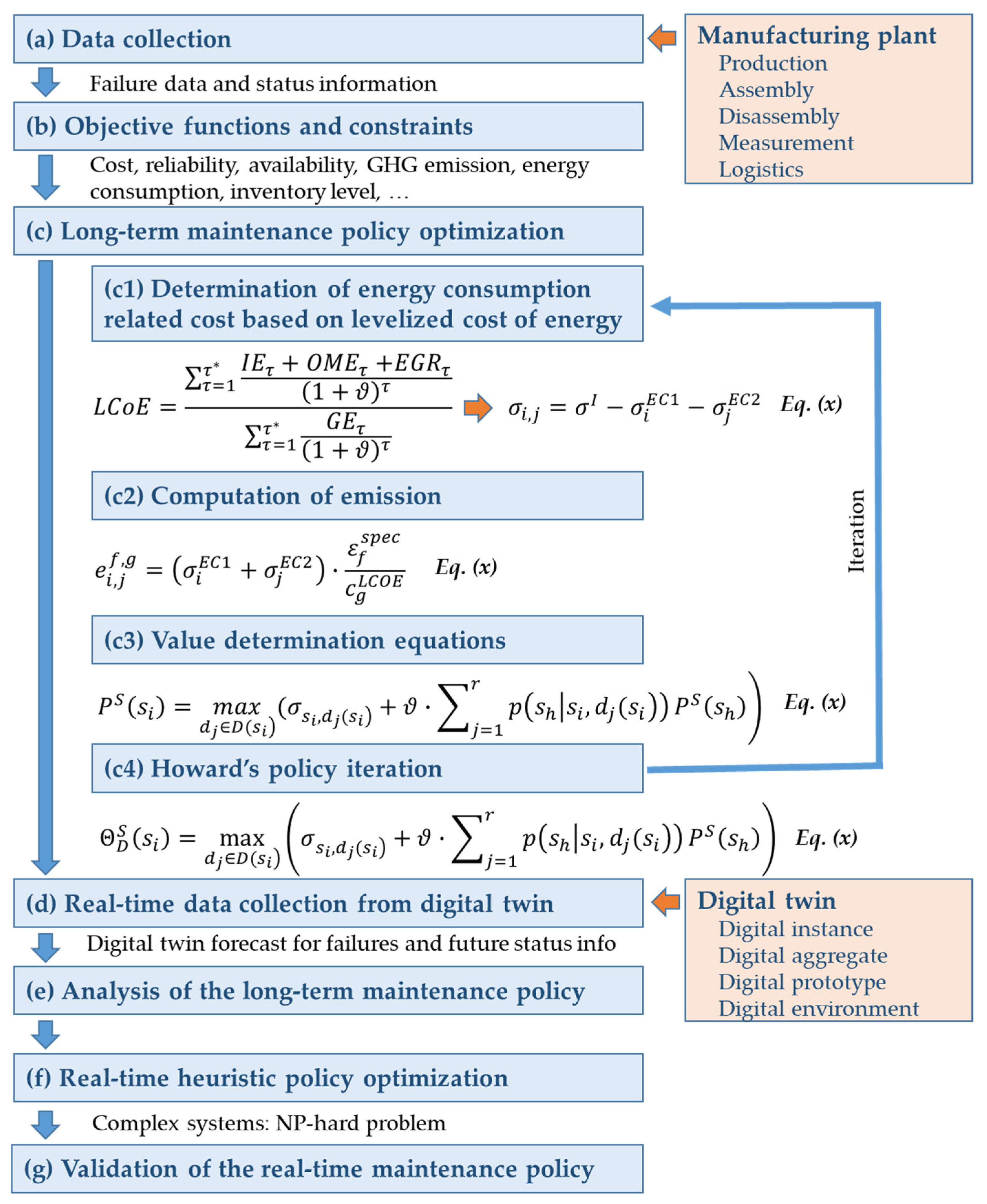
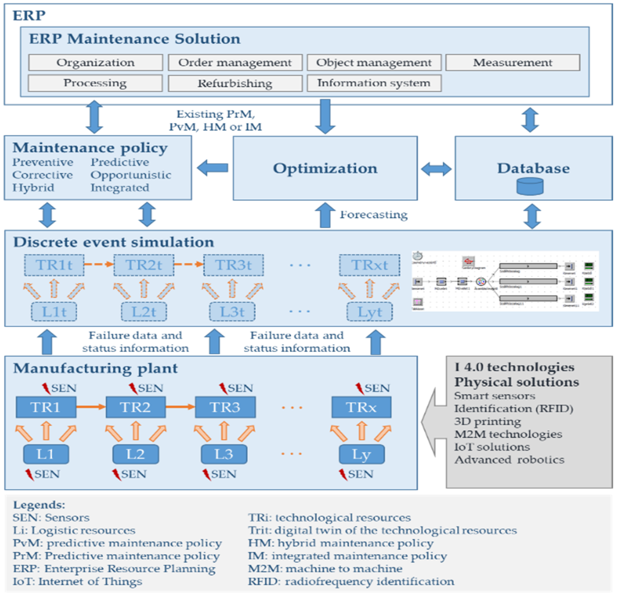
The optimization algorithm is based on the information from the ERP maintenance module, the database of the whole ERP, information from the physical manufacturing and logistics system, and the results of discrete event simulation based on digital twin-information. The functional model of the proposed maintenance optimization is shown in Figure 5.

The manufacturing plant can be divided into two main parts; the first part is the manufacturing system with technological resources, while the second part is the logistics system including devices and logistics resources for loading and unloading, transporting, storage, packaging, and other material handling operations. The fourth industrial revolution makes it possible to transfer conventional manufacturing systems into cyber-physical systems using Industry 4.0 technologies. In the field of technological resources, the most important I4.0 technologies are smart sensors, identification technologies, machine to machine solutions (M2M), advanced robotics, and IoT solutions. The technological part of the manufacturing plant can include intelligent tools and intelligent products; they can link the physical technological resources to the digital twin model. In the same way, the logistics resources, material handling machines can be linked with smart sensors to the digital twin. The smart sensors send failure data and status information from the physical system to the digital twin and based on these data it is possible to forecast the future failures and status of the whole system. The digital twin solution can integrate process simulation, while big data problems can be solved with three different levels of data processing. These three levels are represented by edge computing, fog computing, and cloud computing.

The digital twin of the manufacturing system is a digital aggregate, which is the integration of digital instances and digital prototypes covered by a digital twin environment. This digital twin can support discrete event simulation with failure data and status information, and the discrete event simulation can forecast the future status of instances. Based on these statuses, it is possible to define the optimal maintenance strategy. In conventional manufacturing systems, maintenance is a part of enterprise resource planning, but it is also possible to integrate the maintenance process into the manufacturing execution system (MES), because maintenance operations are close to the operational level and MES can be directly connected to the maintenance operators. The MES makes the correlation between production and maintenance data stronger [65].

The primary benefit of the application of energy efficient maintenance policy optimization is a reduction of energy cost. Energy efficiency and environmental performance are linked to each other. In this approach, energy centered maintenance is taken into consideration, but in the literature [66] there are other types of maintenance approaches (reliability centered maintenance or total productive maintenance).

The reduction of energy consumption of the technological and logistic resources (machine tools and material handling machines) can lead to significant savings in energy costs. Therefore, it is important to find the optimal maintenance policy and maintenance operation schedule. This digital twin-based model makes it possible to perform a maintenance strategy optimization: the maintenance policy optimization is a long-term optimization which is based on Howard’s policy iteration method [67].

3.2. Mathematical Model and Solution of Maintenance Policy Optimization

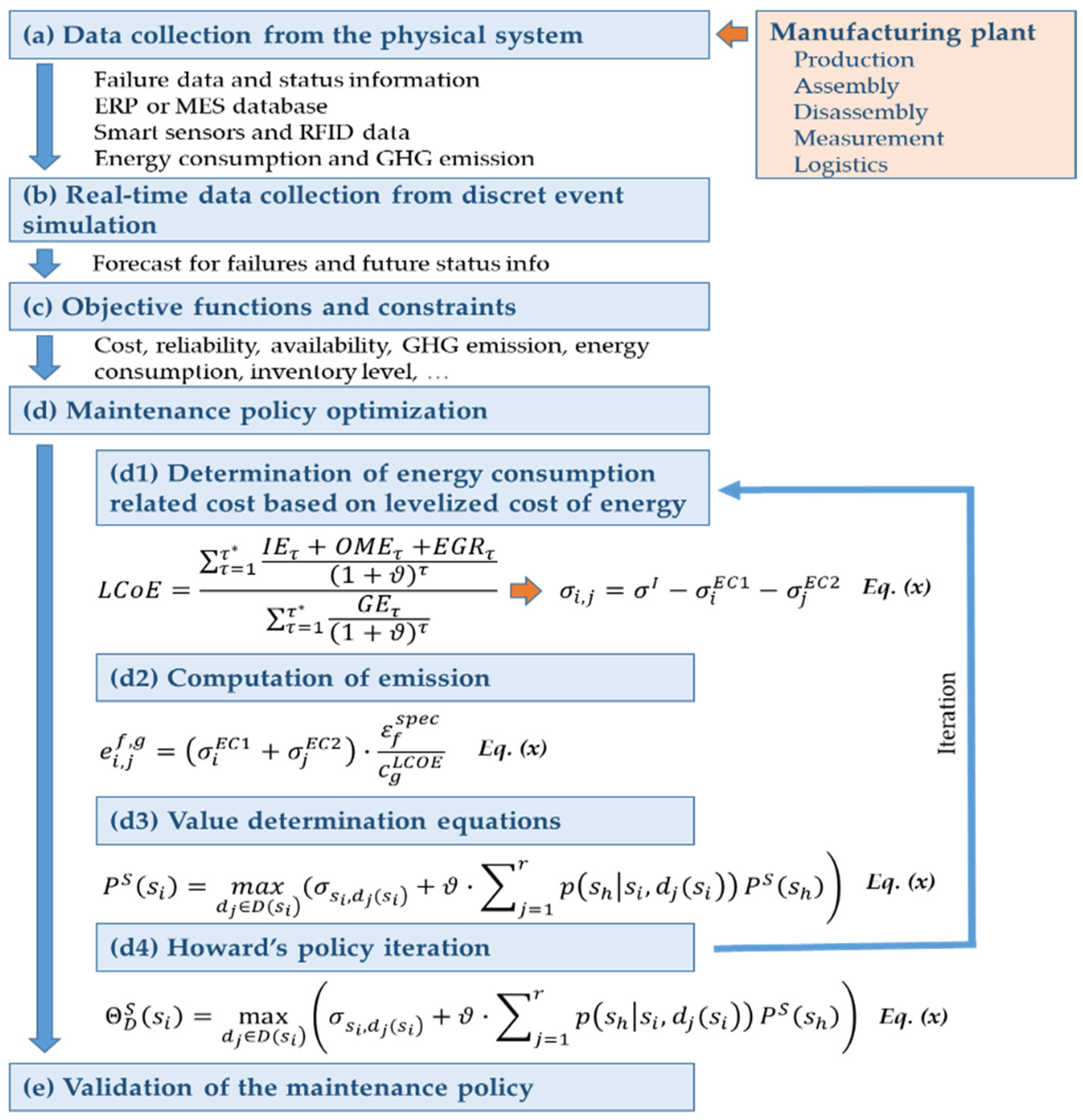
Based on the above described functional model, the digital twin-based maintenance policy optimization process has the following main phases: (a) data collection from the physical system and transformation of data to the digital twin; (b) collection of real-time failure data and status information from the digital twin and discrete event simulation scenarios, especially focusing on energy consumption, emissions, and sustainability aspects; (c) definition of objective functions and constraints of the maintenance strategy; (d) optimization of the maintenance policy based on Howard’s policy iteration method and value determination equations. This optimization phase includes the determination of energy consumption related costs based on the levelized cost of energy, while GHG emission can also be calculated based on the different potential electricity generation sources. The optimization process is shown in Figure 6.

The status of technological and logistics resources can be described as a discrete-time stochastic process; therefore, Markov chains offer suitable representations for the description of this process. The goal of this maintenance policy optimization problem represented by a Markov process is to identify an optimal policy for the decision maker, which can be represented as a set function (see Equation (2)) which specifies the action that the decision maker will choose when the system is in a defined status. A policy is optimal if it minimizes some cumulative function of the random costs, typically the discounted sum over a predefined time window, which can be an infinite time horizon: ${{\displaystyle \sum }}_{\tau =0}^{\infty }={\vartheta }^{\tau }·C\left(D,\tau \right)$, where $C\left(D,\tau \right)$ is the cost at time τ when the decision maker follows policy D, and $\vartheta$ is the discount rate. This Markov decision problem is the infinite-horizon discounted Markov decision problem, which can be solved in many ways: Bellman’s successive approximations method or Howard’s policy iteration.

The benefits of the solution of the mentioned Markov decision process with Howard’s policy iteration techniques for energy consumption are as follows:

• the energy consumption and emissions of the resources in the manufacturing system depends on their status; therefore, the iterated policies using Howard’s methodology can lead to decreased energy consumption and emissions;
• the energy consumption costs of operation and maintenance influences the discounted profit, therefore Howard’s methodology results in optimal maintenance policies from an energy point of view.

The characteristics of the maintenance policy optimization problem is an assignment problem, where suitable maintenance operations have to be assigned to every status of the system resources. As assumptions, the following are taken into consideration.

In the maintenance model we can define a set of possible states:

$$S=\left(s_1,s_2,\cdots ,s_i,\cdots s_z\right).$$

(1)

where $s_i$ is state i of the system and z is the maximum number of possible states of the system. These states have great impact on the energy efficiency of the manufacturing system, which means that this set of possible states also defines a link between status information, maintenance operations, and energy.

This set includes all potential states of the system and these states can be identified either from the failure data and status information of the physical manufacturing and logistics system or from their digital twin aggregate. In the same way, it is possible to define a decision set, which includes all potential decisions regarding the various states of the system. The decision set includes all suitable maintenance processes:

$$D=\left(d_1,d_2,\cdots ,d_j,\cdots d_r\right).$$

(2)

where $d_j$ is potential decision j regarding a maintenance request and r is the maximum number of possible decisions regarding the maintenance of the whole system. These decisions regarding maintenance operations also form a link to the energy consumption, because it is possible to calculate the energy consumption of all maintenance operations.

The transition probabilities represent the constraints of the maintenance policy optimization: $\mathsf{\Gamma }=\left[{\gamma }_{ih}\right]$, where ${\gamma }_{ih}$ is the transition probability from state $s_i$ to state $s_h$ and

$$\forall h:{{\displaystyle \sum }}_{i=1}^z{\gamma }_{ih}=1$$

(3)

The transition probabilities for transition from state $s_i$ to state $s_h$ resulting from decision $d_j$: $p\left(s_h|s_i,d_j\right)$ can be calculated. The following constraints can be defined for the transition probability values:

$$p\left(s_h|s_i,d_j\right)\in \mathsf{\Gamma }\wedge p\left(s_h|s_i,d_j\right)\le {\gamma }_{ih}\vee p\left(s_h|s_i,d_j\right)\ge {\gamma }_{ih},$$

(4)

which means that the chosen decision $d_j$ will not definitely result in the transition probability ${\gamma }_{ih}$ from state $s_i$ to state $s_h$, because $d_j$ will result in a new state of the system and $p\left(s_h|s_i,d_j\right)$ can be defined as the transition probability from the state resulting from the decision $d_j$, from state $s_i$ to the state $s_h$.

Within the frame of the maintenance policy optimization, different objective functions can be taken into consideration: cost, reliability, availability, GHG emission, energy consumption, inventory value, or level of spare parts. In the case of multiple criteria decision making (MCDM), it is possible to involve more than one objective function to be optimized simultaneously. In the case of MCDM, different techniques are used for weighting multiple objectives, the well-known methods are the Churchmann–Ackoff method and the Guilford method. Within the frame of our multi-stage maintenance policy optimization the profit will be used as the objective function of the policy optimization.

In this model, the discounted profit caused by the energy consumption of the manufacturing system and the energy consumption of the maintenance process for an infinite time horizon are taken into consideration. As Winston defines [68], infinite-horizon probabilistic dynamic programing problems are Markov decision processes, where the profit-based objective function can be defined in the following form:

$$P^S\left(s_i\right)=\underset{d_j\in D(s_i)}{max}\left({\sigma }_{s_i,d_j(s_i)}+\vartheta ·{{\displaystyle \sum }}_{j=1}^{r}p\left(s_h|s_i,d_j(s_i)\right)P^S\left(s_h\right)\right),$$

(5)

where ${\sigma }_{s_i,d_j(s_i)}$ is the expected profit in the initial period if decision $d_j$ was chosen for status $s_i$, $P^S\left(s_i\right)$ is the expected discounted profit of status $s_i$, $\vartheta$ is the discounting factor of the profits and $0<\vartheta \le 1$.

The Howard’s policy iteration method is a suitable technique to optimize policies from a value (or cost) determination equation point of view. In this technique, it is possible to calculate a special parameter of the chosen maintenance policy:

$${\mathsf{\Theta }}_D^S\left(s_i\right)=\underset{d_j\in D(s_i)}{\max }\left({\sigma }_{s_i,d_j(s_i)}+\vartheta ·{{\displaystyle \sum }}_{j=1}^{r}p\left(s_h|s_i,d_j(s_i)\right)P^S\left(s_h\right)\right),$$

(6)

where ${\mathsf{\Theta }}_D^S\left(s_i\right)$ is a special parameter of the Howard’s policy iteration technique for the state $s_i$ of the system. If ${\mathsf{\Theta }}_D^S\left(s_i\right)=P^S\left(s_i\right)$ for $j=1\cdots r,$ then $D$ is the optimal maintenance policy, otherwise the policy must be changed and a new iteration phase must be computed using value determination equations and the Howard’s policy iteration parameter calculation.

4. Computational Results

This section discusses a scenario analysis, which focuses on the validation of the above-described multi-phase maintenance policy optimization including the long-term optimization based on Howard’s policy iteration techniques. In this scenario, the manufacturing system has five different statuses (excellent, good, average, poor, and bad), and based on these states the set of possible statuses is given as follows:

$$S=\left(E,G,A,P,B\right).$$

(7)

The decision set of this scenario includes four different level of maintenance policy (no maintenance, level 1, level 2, and level 3):

$$D=\left(NO,L_1,L_2,L_3\right).$$

(8)

The status of the system in the next period depends on the status of the current period, therefore it is possible to define the transition probabilities between statuses as a transition matrix of the Markov decision process:

$$\begin{array}{c}{\gamma }_{E\to E}=0.6,{\gamma }_{E\to G}=0.3,{\gamma }_{E\to A}=0.1,{\gamma }_{G\to G}=0.7,{\gamma }_{G\to A}=0.25,{\gamma }_{G\to P}=0.05\\ {\gamma }_{A\to A}=0.7,{\gamma }_{A\to P}=0.2,{\gamma }_{A\to B}=0.1,{\gamma }_{P\to P}=0.65,{\gamma }_{P\to B}=0.35,{\gamma }_{B\to B}=1.00\end{array}$$

(9)

After performing a maintenance process, the transition probabilities from the current status to status E can be calculated as follows:

$$\begin{array}{c}p\left(E|G,L_1\right)=p\left(E|A,L_2\right)=p\left(E|P,L_3\right)=p\left(E|B,L_4\right)={\gamma }_{E\to E}=0.6\\ p\left(G|G,L_1\right)=p\left(G|A,L_2\right)=p\left(G|P,L_3\right)=p\left(G|B,L_4\right)={\gamma }_{E\to G}=0.3\\ p\left(A|G,L_1\right)=p\left(A|A,L_2\right)=p\left(A|P,L_3\right)=p\left(A|B,L_4\right)={\gamma }_{E\to A}=0.1\\ p\left(P|G,L_1\right)=p\left(P|A,L_2\right)=p\left(P|P,L_3\right)=p\left(P|B,L_4\right)={\gamma }_{E\to P}=0\\ p\left(B|G,L_1\right)=p\left(B|A,L_2\right)=p\left(B|P,L_3\right)=p\left(B|B,L_4\right)={\gamma }_{E\to B}=0\end{array}$$

(10)

After performing a maintenance process, the transition probabilities from the current status to status G can be calculated as follows:

$$\begin{array}{c}p\left(G|A,L_1\right)=p\left(G|P,L_2\right)=p\left(G|B,L_3\right)={\gamma }_{G\to G}=0.7\\ p\left(A|A,L_1\right)=p\left(A|P,L_2\right)=p\left(A|B,L_3\right)={\gamma }_{G\to A}=0.25\\ p\left(P|A,L_1\right)=p\left(P|P,L_2\right)=p\left(P|B,L_3\right)={\gamma }_{G\to P}=0.05\\ p\left(B|A,L_1\right)=p\left(B|P,L_2\right)=p\left(B|B,L_3\right)={\gamma }_{G\to B}=0\end{array}$$

(11)

After performing a maintenance process, the transition probabilities from the current status to status A can be calculated as follows:

$$\begin{array}{c}p\left(A|P,L_1\right)=p\left(A|B,L_2\right)={\gamma }_{A\to A}=0.7\\ p\left(P|P,L_1\right)=p\left(P|B,L_2\right)={\gamma }_{A\to P}=0.2\\ p\left(B|P,L_1\right)=p\left(B|B,L_2\right)={\gamma }_{A\to B}=0.1\end{array}$$

(12)

After performing a maintenance process, the transition probabilities from the current status to status P can be calculated as follows:

$$p\left(P|B,L_1\right)={\gamma }_{P\to P}=0.65$$

(13)

The profit of the analyzed time window of the manufacturing process is influenced by the income and the costs, including energy consumption (electricity) of manufacturing and maintenance:

$${\sigma }_{i,j}={\sigma }^I-{\sigma }_i^{EC1}-{\sigma }_j^{EC2}$$

(14)

where ${\sigma }_{i,j}$ is the profit of the system in the status of the system i, while maintenance level j is performed, ${\sigma }^I$. is the initial income of the manufacturing system, ${\sigma }_i^{EC1}$ is the energy consumption of the manufacturing system in the status i and ${\sigma }_j^{EC2}$. is the energy consumption of the performed maintenance operations of maintenance level j.

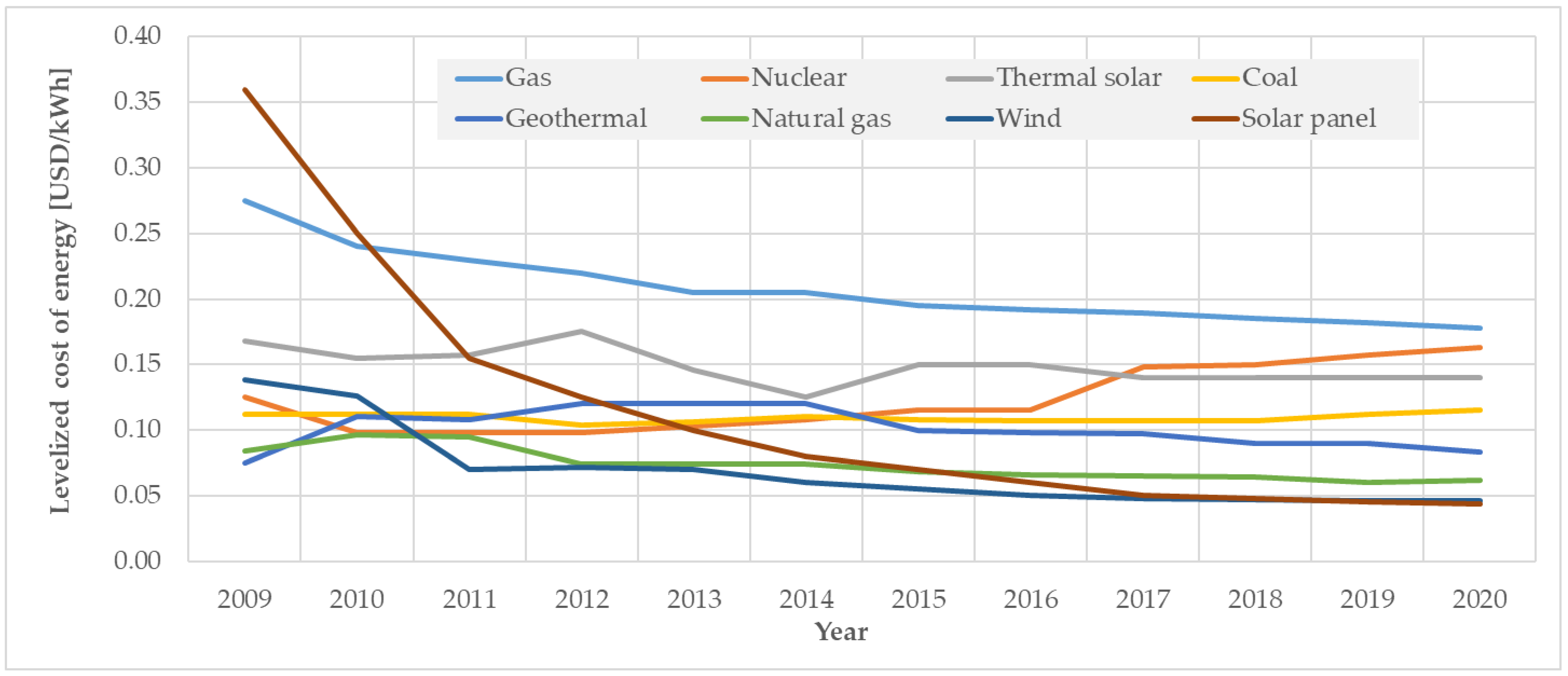
The energy of manufacturing and maintenance operations can be generated from different sources (lignite, coal, oil, natural gas, photovoltaic, biomass, nuclear, water, and wind), and, depending on these energy generation sources, it is possible to calculate both the cost of energy consumption and the virtual emissions of the whole manufacturing process depending on the status of the system and the performed maintenance operations of the chosen maintenance policy. The cost calculation of energy consumption is based on the levelized cost of energy (Figure 7).

The profit of the system based on the status of the system, the performed maintenance level and the costs caused by the energy consumption of the related maintenance level, and the energy consumption of the manufacturing system in the current status are input parameters of the optimization problem:

$$\begin{array}{c}{\sigma }_{E,NO}={\sigma }^I-{\sigma }_E^{EC1}-{\sigma }_{NO}^{EC2}=300{\sigma }_{G,NO}={\sigma }^I-{\sigma }_G^{EC1}-{\sigma }_{NO}^{EC2}=200\\ {\sigma }_{A,NO}={\sigma }^I-{\sigma }_A^{EC1}-{\sigma }_{NO}^{EC2}=100{\sigma }_{P,NO}={\sigma }^I-{\sigma }_P^{EC1}-{\sigma }_{NO}^{EC2}=20\\ {\sigma }_{B,NO}={\sigma }^I-{\sigma }_B^{EC1}-{\sigma }_{NO}^{EC2}=10{\sigma }_{G,L1}={\sigma }^I-{\sigma }_E^{EC1}-{\sigma }_{L1}^{EC2}=190\\ {\sigma }_{A,L1}={\sigma }^I-{\sigma }_G^{EC1}-{\sigma }_{L1}^{EC2}=90{\sigma }_{P,L1}={\sigma }^I-{\sigma }_A^{EC1}-{\sigma }_{L1}^{EC2}=-10\\ {\sigma }_{B,L1}={\sigma }^I-{\sigma }_P^{EC1}-{\sigma }_{L1}^{EC2}=-90{\sigma }_{A,L2}={\sigma }^I-{\sigma }_E^{EC1}-{\sigma }_{L2}^{EC2}=170\\ {\sigma }_{P,L2}={\sigma }^I-{\sigma }_G^{EC1}-{\sigma }_{L2}^{EC2}=70{\sigma }_{B,L2}={\sigma }^I-{\sigma }_A^{EC1}-{\sigma }_{L2}^{EC2}=-30\\ {\sigma }_{P,L3}={\sigma }^I-{\sigma }_E^{EC1}-{\sigma }_{L3}^{EC2}=-100{\sigma }_{B,L3}={\sigma }^I-{\sigma }_G^{EC1}-{\sigma }_{L3}^{EC2}=-200\end{array}$$

(15)

For this calculation, the initial energy consumption of manufacturing and maintenance is taken into consideration (

Table 1. Initial energy consumption of manufacturing and maintenance operations in MW within one cycle of the time window of the analysis.

Status of the System 1	E	G	A	P	B
Energy consuption	10.483	12.096	13.709	15.000	15.161

¹ E = Excellent, G = good, A = average, P = poor, B = bad.

and

Table 2. Initial energy consumption of different maintenance policies in MW within one cycle of the time window of the analysis.

Maintenance Policy 1	NO	L1	L2	L3
Energy consuption	0	1.774	2.096	6.451

¹ NO = No maintenance, L1 = level 1 maintenance, L2 = level 2 maintenance, L3 = level 3 maintenance.

).

In this model, the greenhouse gas emissions of various electricity generations sources published by World Nuclear Association are taken into consideration [69].

Based on the specific GHG emission (

Table 3. Specific greenhouse gas (GHG) emission depending on the electricity generation source in CO₂ emission in g/kWh. [69].

EGS 1	Emission
	CO2	SO2	CO	HC	NOX	PM
Lignite	1054	0.032	0.880	0.480	4.760	0.040
Coal	888	0.028	0.733	0.400	3.960	0.030
Oil	733	0.022	0.615	0.335	3.324	0.028
Natural gas	499	0.016	0.418	0.228	2.226	0.019
Photovoltaic	85	0.002	0.073	0.040	0.396	0.003
Biomass	45	0.001	0.038	0.021	0.205	0.002
Nuclear	29	<10−3	0.024	0.013	0.132	0.001
Water	26	<10−3	0.022	0.012	0.119	0.001
Wind	26	<10−3	0.022	0.012	0.119	0.001

¹ EGS = Electricity Generation Source.

), the total virtual GHG emission can be calculated based on the status of the manufacturing system and the chosen maintenance policy:

$$e_{i,j}^{f,g}=\left({\sigma }_i^{EC1}+{\sigma }_j^{EC2}\right)·\frac{{\epsilon }_f^{spec}}{c_g^{LCOE}}$$

(16)

where $e_{i,j}^{f,g}$ is the virtual emission of GHG f in the case of the state i of manufacturing system, chosen maintenance policy j, and electricity generation source g, ${\epsilon }_f^{spec}$ is the specific GHG emission of GHG f, $c_g^{LCOE}$ is the levelized cost of electricity in the case of electricity generation source g, where $f\in \left(C{O}_2,S{O}_2,CO,HC,N{O}_X,PM\right)$.

The virtual GHG emission in the case of natural gas electricity generation source is shown in

Table 4. Computational results of virtual CO₂ emission in kg within one cycle of the time-window of analysis.

		${\mathit{\sigma }}_{\mathit{j}}^{\mathit{E}\mathit{C}2}$
		${\mathit{\sigma }}_{\mathit{N}\mathit{O}}^{\mathit{E}\mathit{C}2}$	${\mathit{\sigma }}_{\mathit{L}1}^{\mathit{E}\mathit{C}2}$	${\mathit{\sigma }}_{\mathit{L}2}^{\mathit{E}\mathit{C}2}$	${\mathit{\sigma }}_{\mathit{L}3}^{\mathit{E}\mathit{C}2}$
	${\sigma }_E^{EC1}$	$e_{E,NO}^{C{O}_2,ng}=5231$	n.a.	n.a.	n.a.
	${\sigma }_G^{EC1}$	$e_{G,NO}^{C{O}_2,ng}=6035$	$e_{G,L1}^{C{O}_2,ng}$ = 6921	n.a.	n.a.
${\sigma }_i^{EC1}$	${\sigma }_A^{EC1}$	$e_{A,NO}^{C{O}_2,ng}$ = 6840	$e_{A,L1}^{C{O}_2,ng}$ = 7726	$e_{A,L2}^{C{O}_2,ng}$ = 7886	n.a.
	${\sigma }_P^{EC1}$	$e_{P,NO}^{C{O}_2,ng}$ = 7485	$e_{P,L1}^{C{O}_2,ng}$ = 8370	$e_{P,L2}^{C{O}_2,ng}$ = 8530	$e_{P,L3}^{C{O}_2,ng}$ = 10,704
	${\sigma }_B^{EC1}$	$e_{B,NO}^{C{O}_2,ng}$ = 7565	$e_{B,L1}^{C{O}_2,ng}$ = 8450	$e_{B,L2}^{C{O}_2,ng}$ = 8611	$e_{B,L3}^{C{O}_2,ng}$ = 10,784

. The computational results regarding the virtual emission of other GHGs are in

Table 5. Computational results of the virtual SO₂ emission in kg within one cycle.

		${\mathit{\sigma }}_{\mathit{j}}^{\mathit{E}\mathit{C}2}$
		${\mathit{\sigma }}_{\mathit{N}\mathit{O}}^{\mathit{E}\mathit{C}2}$	${\mathit{\sigma }}_{\mathit{L}1}^{\mathit{E}\mathit{C}2}$	${\mathit{\sigma }}_{\mathit{L}2}^{\mathit{E}\mathit{C}2}$	${\mathit{\sigma }}_{\mathit{L}3}^{\mathit{E}\mathit{C}2}$
	${\sigma }_E^{EC1}$	$e_{E,NO}^{S{O}_2,ng}=0.166$	n.a.	n.a.	n.a.
	${\sigma }_G^{EC1}$	$e_{G,NO}^{S{O}_2,ng}=0.193$	$e_{G,L1}^{S{O}_2,ng}$ = 0.221	n.a.	n.a.
${\sigma }_i^{EC1}$	${\sigma }_A^{EC1}$	$e_{A,NO}^{S{O}_2,ng}$ = 0.219	$e_{A,L1}^{S{O}_2,ng}$ = 0.247	$e_{A,L2}^{S{O}_2,ng}$ = 0.253	n.a.
	${\sigma }_P^{EC1}$	$e_{P,NO}^{S{O}_2,ng}$ = 0.240	$e_{P,L1}^{S{O}_2,ng}$ = 0.268	$e_{P,L2}^{S{O}_2,ng}$ = 0.274	$e_{P,L3}^{S{O}_2,ng}$ = 0.343
	${\sigma }_B^{EC1}$	$e_{B,NO}^{S{O}_2,ng}$ = 0.243	$e_{B,L1}^{S{O}_2,ng}$ = 0.271	$e_{B,L2}^{S{O}_2,ng}$ = 0.276	$e_{B,L3}^{S{O}_2,ng}$ = 0.346

,

Table 6. Computational results of the virtual CO emission in kg within one cycle.

		${\mathit{\sigma }}_{\mathit{j}}^{\mathit{E}\mathit{C}2}$
		${\mathit{\sigma }}_{\mathit{N}\mathit{O}}^{\mathit{E}\mathit{C}2}$	${\mathit{\sigma }}_{\mathit{L}1}^{\mathit{E}\mathit{C}2}$	${\mathit{\sigma }}_{\mathit{L}2}^{\mathit{E}\mathit{C}2}$	${\mathit{\sigma }}_{\mathit{L}3}^{\mathit{E}\mathit{C}2}$
	${\sigma }_E^{EC1}$	$e_{E,NO}^{CO,ng}=4.382$	n.a.	n.a.	n.a.
	${\sigma }_G^{EC1}$	$e_{G,NO}^{CO,ng}=5.056$	$e_{G,L1}^{CO,ng}$ = 5.797	n.a.	n.a.
${\sigma }_i^{EC1}$	${\sigma }_A^{EC1}$	$e_{A,NO}^{CO,ng}$ = 5.730	$e_{A,L1}^{CO,ng}$ = 6.472	$e_{A,L2}^{CO,ng}$ = 6.606	n.a.
	${\sigma }_P^{EC1}$	$e_{P,NO}^{CO,ng}$ = 6.270	$e_{P,L1}^{CO,ng}$ = 7.012	$e_{P,L2}^{CO,ng}$ = 7.146	$e_{P,L3}^{CO,ng}$ = 8.966
	${\sigma }_B^{EC1}$	$e_{B,NO}^{CO,ng}$ = 6.337	$e_{B,L1}^{CO,ng}$ = 7.079	$e_{B,L2}^{CO,ng}$ = 7.213	$e_{B,L3}^{CO,ng}$ = 9.034

,

Table 7. Computational results of the virtual HC emission in kg within one cycle.

		${\mathit{\sigma }}_{\mathit{j}}^{\mathit{E}\mathit{C}2}$
		${\mathit{\sigma }}_{\mathit{N}\mathit{O}}^{\mathit{E}\mathit{C}2}$	${\mathit{\sigma }}_{\mathit{L}1}^{\mathit{E}\mathit{C}2}$	${\mathit{\sigma }}_{\mathit{L}2}^{\mathit{E}\mathit{C}2}$	${\mathit{\sigma }}_{\mathit{L}3}^{\mathit{E}\mathit{C}2}$
	${\sigma }_E^{EC1}$	$e_{E,NO}^{HC,ng}=2.390$	n.a.	n.a.	n.a.
	${\sigma }_G^{EC1}$	$e_{G,NO}^{HC,ng}=2.757$	$e_{G,L1}^{HC,ng}$ = 3.162	n.a.	n.a.
${\sigma }_i^{EC1}$	${\sigma }_A^{EC1}$	$e_{A,NO}^{HC,ng}$ = 3.125	$e_{A,L1}^{HC,ng}$ = 3.530	$e_{A,L2}^{HC,ng}$ = 3.603	n.a.
	${\sigma }_P^{EC1}$	$e_{P,NO}^{HC,ng}$ = 3.420	$e_{P,L1}^{HC,ng}$ = 3.824	$e_{P,L2}^{HC,ng}$ = 3.897	$e_{P,L3}^{HC,ng}$ = 4.891
	${\sigma }_B^{EC1}$	$e_{B,NO}^{HC,ng}$ = 3.457	$e_{B,L1}^{HC,ng}$ = 3.861	$e_{B,L2}^{HC,ng}$ = 3.934	$e_{B,L3}^{HC,ng}$ = 4.928

,

Table 8. Computational results of the virtual NO_x emission in kg within one cycle.

		${\mathit{\sigma }}_{\mathit{j}}^{\mathit{E}\mathit{C}2}$
		${\mathit{\sigma }}_{\mathit{N}\mathit{O}}^{\mathit{E}\mathit{C}2}$	${\mathit{\sigma }}_{\mathit{L}1}^{\mathit{E}\mathit{C}2}$	${\mathit{\sigma }}_{\mathit{L}2}^{\mathit{E}\mathit{C}2}$	${\mathit{\sigma }}_{\mathit{L}3}^{\mathit{E}\mathit{C}2}$
	${\sigma }_E^{EC1}$	$e_{E,NO}^{N{O}_x,ng}=23.335$	n.a.	n.a.	n.a.
	${\sigma }_G^{EC1}$	$e_{G,NO}^{N{O}_x,ng}=26.925$	$e_{G,L1}^{N{O}_x,ng}$ = 30.874	n.a.	n.a.
${\sigma }_i^{EC1}$	${\sigma }_A^{EC1}$	$e_{A,NO}^{N{O}_x,ng}$ = 30.516	$e_{A,L1}^{N{O}_x,ng}$ = 34.465	$e_{A,L2}^{N{O}_x,ng}$ = 35.181	n.a.
	${\sigma }_P^{EC1}$	$e_{P,NO}^{N{O}_x,ng}$ = 33.390	$e_{P,L1}^{N{O}_x,ng}$ = 37.339	$e_{P,L2}^{N{O}_x,ng}$ = 38.055	$e_{P,L3}^{N{O}_x,ng}$ = 47.749
	${\sigma }_B^{EC1}$	$e_{B,NO}^{N{O}_x,ng}$ = 33.748	$e_{B,L1}^{N{O}_x,ng}$ = 37.697	$e_{B,L2}^{N{O}_x,ng}$ = 38.414	$e_{B,L3}^{N{O}_x,ng}$ = 48.108

and

Table 9. Computational results of the virtual PM emission in kg within one cycle.

		${\mathit{\sigma }}_{\mathit{j}}^{\mathit{E}\mathit{C}2}$
		${\mathit{\sigma }}_{\mathit{N}\mathit{O}}^{\mathit{E}\mathit{C}2}$	${\mathit{\sigma }}_{\mathit{L}1}^{\mathit{E}\mathit{C}2}$	${\mathit{\sigma }}_{\mathit{L}2}^{\mathit{E}\mathit{C}2}$	${\mathit{\sigma }}_{\mathit{L}3}^{\mathit{E}\mathit{C}2}$
	${\sigma }_E^{EC1}$	$e_{E,NO}^{PM,ng}=0.199$	n.a.	n.a.	n.a.
	${\sigma }_G^{EC1}$	$e_{G,NO}^{PM,ng}=0.229$	$e_{G,L1}^{PM,ng}$ = 0.263	n.a.	n.a.
${\sigma }_i^{EC1}$	${\sigma }_A^{EC1}$	$e_{A,NO}^{PM,ng}$ = 0.260	$e_{A,L1}^{PM,ng}$ = 0.294	$e_{A,L2}^{PM,ng}$ = 0.300	n.a.
	${\sigma }_P^{EC1}$	$e_{P,NO}^{PM,ng}$ = 0.285	$e_{P,L1}^{PM,ng}$ = 0.318	$e_{P,L2}^{PM,ng}$ = 0.324	$e_{P,L3}^{PM,ng}$ = 0.407
	${\sigma }_B^{EC1}$	$e_{B,NO}^{PM,ng}$ = 0.288	$e_{B,L1}^{PM,ng}$ = 0.321	$e_{B,L2}^{PM,ng}$ = 0.327	$e_{B,L3}^{PM,ng}$ = 0.411

.

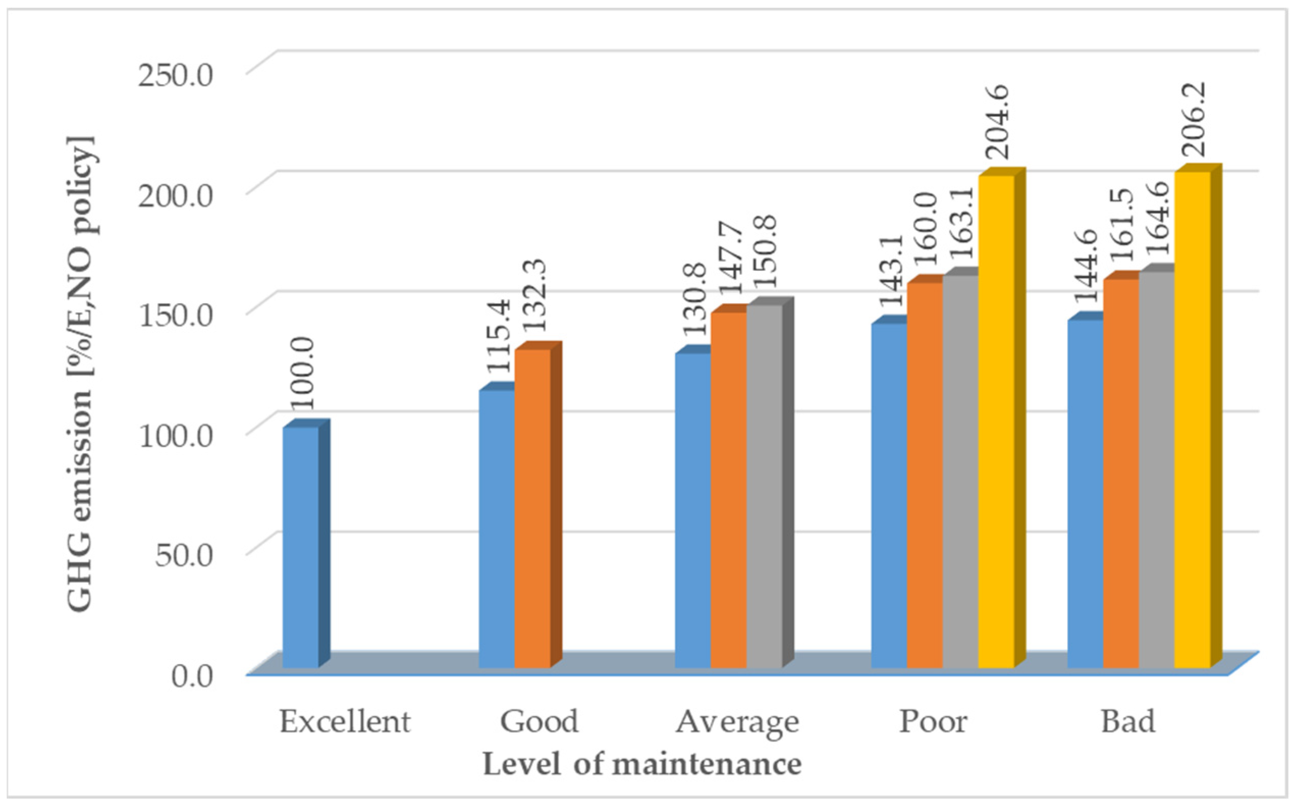
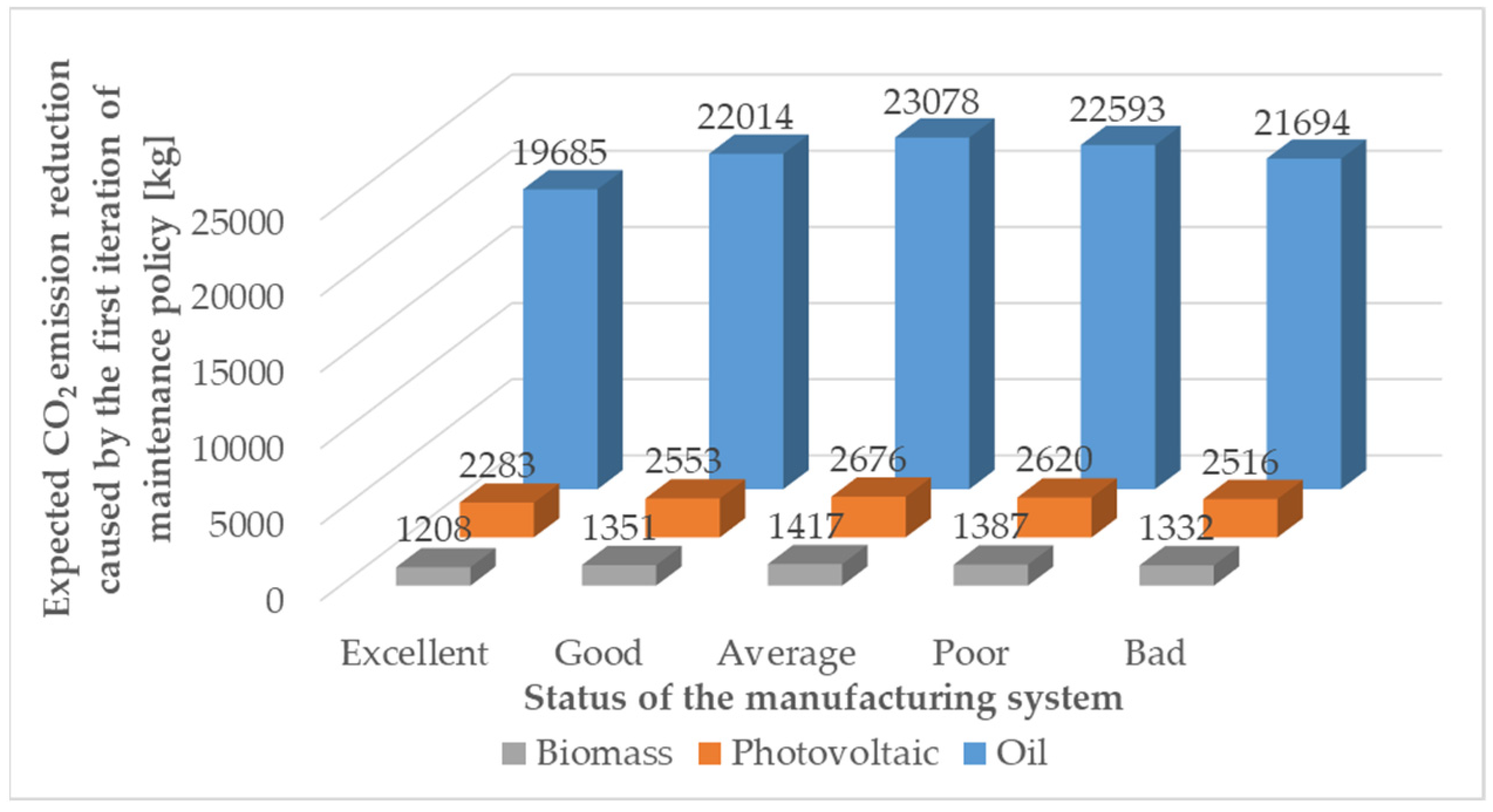
As the above tables show, the GHG emission depends on the status of the systems and the maintenance operations performed. The resulting proportion of GHG emission is shown in Figure A1. The expected CO₂ emission reduction caused by the first iteration of the maintenance policy [kg] is shown in Figure A2. After the initialization of the energy consumption and GHG emission values, the first step is to choose an initial maintenance policy:

$$S^{*}\left(E\right)=NO,S^{*}\left(G\right)=NO,S^{*}\left(A\right)=L_1,S^{*}\left(P\right)=L_1,S^{*}\left(B\right)=L_2,$$

(17)

which means that in the case of status E and status G no maintenance is performed, in the case of status A and P first level maintenance is performed, and in the case of status B second level maintenance is chosen. The value determination equations (see Equation (5)), and the expected discounted profit for the predefined time-window can be calculated as follows:

$$\begin{array}{c}{P}^{S^{*}}\left(E\right)={\sigma }_{E,NO}+\vartheta ·\left({\gamma }_{E\to E}·P^{S^{*}}\left(E\right)+{\gamma }_{E\to G}·P^{S^{*}}\left(G\right)+{\gamma }_{E\to A}·P^{S^{*}}\left(A\right)\right)\\ P^{S^{*}}\left(G\right)={\sigma }_{G,NO}+\vartheta ·\left({\gamma }_{G\to G}·P^{S^{*}}\left(G\right)+{\gamma }_{G\to A}·P^{S^{*}}\left(A\right)+{\gamma }_{G\to P}·P^{S^{*}}\left(P\right)\right)\\ P^{S^{*}}\left(A\right)={\sigma }_{A,NO}+\vartheta ·\left({\gamma }_{G\to G}·P^{S^{*}}\left(G\right)+{\gamma }_{G\to A}·P^{S^{*}}\left(A\right)+{\gamma }_{G\to P}·P^{S^{*}}\left(P\right)\right)\\ P^{S^{*}}\left(P\right)={\sigma }_{P,NO}+\vartheta ·\left({\gamma }_{A\to A}·P^{S^{*}}\left(A\right)+{\gamma }_{A\to P}·P^{S^{*}}\left(P\right)+{\gamma }_{A\to B}·P^{S^{*}}\left(B\right)\right)\\ P^{S^{*}}\left(B\right)={\sigma }_{B,NO}+\vartheta ·\left({\gamma }_{A\to A}·P^{S^{*}}\left(A\right)+{\gamma }_{A\to P}·P^{S^{*}}\left(P\right)+{\gamma }_{A\to B}·P^{S^{*}}\left(B\right)\right)\end{array}$$

(18)

Solving these equations, the expected discounted profit for each status in the case of the initial maintenance policy can be determined:

$$\begin{array}{c}{P}^{S^{*}}\left(E\right)=3461.43€P^{S^{*}}\left(G\right)=3154.9€P^{S^{*}}\left(A\right)=3044.9€\\ P^{S^{*}}\left(P\right)=2815.33€P^{S^{*}}\left(B\right)=2795.33€\end{array}$$

(19)

After the solution of value determination equations, the next phase is to apply the Howard’s policy iteration technique, and calculate a ${\mathsf{\Theta }}^{S^{*}}$ parameter for each $S^{*}$ maintenance policy. In the case of status E no maintenance is required, therefore based on Equation (6) it is meaningless to change the maintenance policy for status E:

$${\mathsf{\Theta }}^{S^{*}}\left(E\right)=P^{S^{*}}\left(E\right)\to S^{**}\left(E\right)=S^{*}\left(E\right)=NO$$

(20)

In the case of status G, the value of ${\mathsf{\Theta }}^{S^{*}}$ parameter can be computed as follows:

$${\mathsf{\Theta }}^{S^{*}}\left(G\right)=max\{\begin{array}{cc}NO:& {\sigma }_{G,NO}+\vartheta ·\left({\gamma }_{G\to G}·P^{S^{*}}\left(G\right)+{\gamma }_{G\to A}·P^{S^{*}}\left(A\right)+{\gamma }_{G\to P}·P^{S^{*}}\left(P\right)\right)\\ L_1:& {\sigma }_{G,L_1}+\vartheta ·\left({\gamma }_{E\to E}·P^{S^{*}}\left(E\right)+{\gamma }_{E\to G}·P^{S^{*}}\left(G\right)+{\gamma }_{E\to A}·P^{S^{*}}\left(A\right)\right)\end{array}$$

(21)

As the solution of Equation (21) shows, ${\mathsf{\Theta }}^{S^{*}}\left(G\right)=3351.43€$, which means, that there is a better maintenance policy, than the initial policy chosen in the first iteration:

$${\mathsf{\Theta }}^{S^{*}}\left(E\right)>P^{S^{*}}\left(E\right)\to S^{**}\left(E\right)\ne S^{*}\left(E\right)\to S^{**}\left(E\right)=L_1$$

(22)

In the case of status A, the value of ${\mathsf{\Theta }}^{S^{*}}$ parameter can be computed as follows:

$$\mathsf{\Theta }^(S^\ast )\left(A\right)=max\{\begin{array}{cc}NO:& {\sigma }_{A,NO}+\vartheta ·\left({\gamma }_{A\to A}·P^{S^{*}}\left(A\right)+{\gamma }_{A\to P}·P^{S^{*}}\left(P\right)+{\gamma }_{A\to B}·P^{S^{*}}\left(B\right)\right)\\ L_1:& {\sigma }_{A,L_1}+\vartheta ·\left({\gamma }_{G\to G}·P^{S^{*}}\left(G\right)+{\gamma }_{G\to A}·P^{S^{*}}\left(A\right)+{\gamma }_{G\to P}·P^{S^{*}}\left(P\right)\right)\\ L_2:& {\sigma }_{A,L_2}+\vartheta ·\left({\gamma }_{E\to E}·P^{S^{*}}\left(E\right)+{\gamma }_{E\to G}·P^{S^{*}}\left(G\right)+{\gamma }_{E\to A}·P^{S^{*}}\left(A\right)\right)\end{array}$$

(23)

As the solution of Equation (23) shows, ${\mathsf{\Theta }}^{S^{*}}\left(A\right)=3331.43€$, which means, that there is a better maintenance policy for status A of the system, than the $S^{*}\left(A\right)=L_1$ initial policy chosen in the first iteration:

$${\mathsf{\Theta }}^{S^{*}}\left(A\right)>P^{S^{*}}\left(A\right)\to S^{**}\left(A\right)\ne S^{*}\left(A\right)\to S^{**}\left(A\right)=L_2$$

(24)

In the case of status P, the value of ${\mathsf{\Theta }}^{S^{*}}$ parameter can be computed as follows:

$${\mathsf{\Theta }}^{S^{*}}\left(P\right)=max\{\begin{array}{cc}NO:& {\sigma }_{P,NO}+\vartheta ·\left({\gamma }_{P\to P}·P^{S^{*}}\left(P\right)+{\gamma }_{P\to B}·P^{S^{*}}\left(B\right)\right)\\ L_1:& {\sigma }_{P,L_1}+\vartheta ·\left({\gamma }_{A\to A}·P^{S^{*}}\left(A\right)+{\gamma }_{A\to P}·P^{S^{*}}\left(P\right)+{\gamma }_{A\to B}·P^{S^{*}}\left(B\right)\right)\\ L_2:& {\sigma }_{P,L_2}+\vartheta ·\left({\gamma }_{G\to G}·P^{S^{*}}\left(G\right)+{\gamma }_{G\to A}·P^{S^{*}}\left(A\right)+{\gamma }_{G\to P}·P^{S^{*}}\left(P\right)\right)\\ L_3:& {\sigma }_{P,L_3}+\vartheta ·\left({\gamma }_{E\to E}·P^{S^{*}}\left(E\right)+{\gamma }_{E\to G}·P^{S^{*}}\left(G\right)+{\gamma }_{E\to A}·P^{S^{*}}\left(A\right)\right)\end{array}$$

(25)

As the solution of Equation (25) shows, ${\mathsf{\Theta }}^{S^{*}}\left(P\right)=3061.43€$, which means, that there is a better maintenance policy for status P of the system, than the $S^{*}\left(P\right)=L_1$ initial policy chosen in the first iteration:

$${\mathsf{\Theta }}^{S^{*}}\left(P\right)>P^{S^{*}}\left(P\right)\to S^{**}\left(P\right)\ne S^{*}\left(P\right)\to S^{**}\left(P\right)=L_3$$

(26)

In the case of status B, the value of ${\mathsf{\Theta }}^{S^{*}}$ parameter can be computed as follows:

$${\mathsf{\Theta }}^{S^{*}}\left(B\right)=max\{\begin{array}{cc}NO:& {\sigma }_{B,NO}+\vartheta ·P^{S^{*}}\left(B\right)\\ L_1:& {\sigma }_{B,L_1}+\vartheta ·\left({\gamma }_{P\to P}·P^{S^{*}}\left(P\right)+{\gamma }_{P\to B}·P^{S^{*}}\left(B\right)\right)\\ L_2:& {\sigma }_{B,L_2}+\vartheta ·\left({\gamma }_{A\to A}·P^{S^{*}}\left(A\right)+{\gamma }_{A\to P}·P^{S^{*}}\left(P\right)+{\gamma }_{A\to B}·P^{S^{*}}\left(B\right)\right)\\ L_3:& {\sigma }_{B,L_3}+\vartheta ·\left({\gamma }_{G\to G}·P^{S^{*}}\left(G\right)+{\gamma }_{G\to A}·P^{S^{*}}\left(A\right)+{\gamma }_{G\to P}·P^{S^{*}}\left(P\right)\right)\end{array}$$

(27)

As the solution of Equation (27) shows, ${\mathsf{\Theta }}^{S^{*}}\left(B\right)=2795.33€$, which means, that there is a better maintenance policy for status P of the system than the $S^{*}\left(B\right)=L_2$ initial policy chosen in the first iteration:

$${\mathsf{\Theta }}^{S^{*}}\left(B\right)>P^{S^{*}}\left(B\right)\to S^{**}\left(B\right)\ne S^{*}\left(B\right)\to S^{**}\left(B\right)=L_2$$

(28)

After that, the new value determination equations can be defined, and the expected discounted profit can be calculated in the case of $S^{**}$ maintenance policy for the predefined time-window:

$$\begin{array}{c}{P}^{S^{**}}\left(E\right)={\sigma }_{E,NO}+\vartheta ·\left({\gamma }_{E\to E}·P^{S^{**}}\left(E\right)+{\gamma }_{E\to G}·P^{S^{**}}\left(G\right)+{\gamma }_{E\to A}·P^{S^{**}}\left(A\right)\right)\\ P^{S^{**}}\left(G\right)={\sigma }_{G,L_1}+\vartheta ·\left({\gamma }_{E\to E}·P^{S^{**}}\left(E\right)+{\gamma }_{E\to G}·P^{S^{**}}\left(G\right)+{\gamma }_{E\to A}·P^{S^{**}}\left(A\right)\right)\\ P^{S^{**}}\left(A\right)={\sigma }_{A,L_2}+\vartheta ·\left({\gamma }_{E\to E}·P^{S^{**}}\left(E\right)+{\gamma }_{E\to G}·P^{S^{**}}\left(G\right)+{\gamma }_{E\to A}·P^{S^{**}}\left(A\right)\right)\\ P^{S^{**}}\left(P\right)={\sigma }_{P,L_3}+\vartheta ·\left({\gamma }_{E\to E}·P^{S^{**}}\left(E\right)+{\gamma }_{E\to G}·P^{S^{**}}\left(G\right)+{\gamma }_{E\to A}·P^{S^{**}}\left(A\right)\right)\\ P^{S^{**}}\left(B\right)={\sigma }_{B,L_2}+\vartheta ·\left({\gamma }_{A\to A}·P^{S^{**}}\left(A\right)+{\gamma }_{A\to P}·P^{S^{**}}\left(P\right)+{\gamma }_{A\to B}·P^{S^{**}}\left(B\right)\right)\end{array}$$

(29)

Solving these equations, the expected profit for each status in the case of the $S^{**}$ first iteration of maintenance policy (see Equation (29)) can be given:

$$\begin{array}{c}{P}^{S^{**}}\left(E\right)=5126€P^{S^{**}}\left(G\right)=5016€P^{S^{**}}\left(A\right)=4996€\\ P^{S^{**}}\left(P\right)=4726€P^{S^{**}}\left(B\right)=4630.14€\end{array}$$

(30)

Based on the results of the $S^{**}$ first iteration, the energy consumption reduction can be determined:

$${\omega }_{i,g}^{*}=\frac{(P_i^{S**}-P_i^{S*})}{c_g^{LCOE}}$$

(31)

where ${\omega }_{i,g}^{*}$ is the energy consumption reduction resulting from the first iteration phase in the case of system status i and electricity generation source g. Similarly, the GHG emission reduction can also be calculated:

$${\zeta }_{i,g,f}^{*}=\frac{(P_i^{S**}-P_i^{S*})}{c_g^{LCOE}}·\frac{{\epsilon }_f^{spec}}{c_g^{LCOE}}$$

(32)

where ${\zeta }_{i,g,f}^{*}$ is the GHG emission reduction resulting from the first iteration phase in the case of system status i, electricity generation source g, and GHG f.

The computational results of energy consumption reduction and GHG emission reduction after the first iteration phase in the case of natural gas electricity generation source are described in

Table 10. Energy consumption reduction and GHG emission reduction resulting from the first iteration of maintenance policy optimization within the whole time-window of analysis in the case of natural gas electricity generation source.

Initial System Status	Energy Consumption Reduction 1	GHG Emission Reduction 2
		CO2	SO2	CO	HC	NOX	PM
E	26,854.84	13,400.565	0.430	11.225	6.123	59.779	0.510
G	30,032.26	14,986.097	0.481	12.553	6.847	66.852	0.571
A	31,483.87	15,710.452	0.504	13.160	7.178	70.083	0.598
P	30,822.58	15,380.468	0.493	12.884	7.028	68.611	0.586
B	29,596.77	14,768.790	0.474	12.371	6.748	65.882	0.562

¹ [kW] ² [kg].

.

After the second solution of the value determination equations, the Howard’s policy iteration techniques can be applied, and the ${\mathsf{\Theta }}^{S^{**}}$ parameter for each $S^{**}$ maintenance policy can be calculated. In the case of status E, no maintenance is required, therefore based on Equation (6) it is meaningless to change the maintenance policy for status E:

$${\mathsf{\Theta }}^{S^{**}}\left(E\right)=P^{S^{**}}\left(E\right)\to S^{***}\left(E\right)=S^{**}\left(E\right)=S^{*}\left(E\right)=NO$$

(33)

In the case of status G, the value of ${\mathsf{\Theta }}^{S^{**}}$ parameter can be computed as follows:

$${\mathsf{\Theta }}^{S^{**}}\left(G\right)=max\{\begin{array}{cc}NO:& {\sigma }_{G,NO}+\vartheta ·\left({\gamma }_{G\to G}·P^{S^{**}}\left(G\right)+{\gamma }_{G\to A}·P^{S^{**}}\left(A\right)+{\gamma }_{G\to P}·P^{S^{**}}\left(P\right)\right)\\ L_1:& {\sigma }_{G,L_1}+\vartheta ·\left({\gamma }_{E\to E}·P^{S^{**}}\left(E\right)+{\gamma }_{E\to G}·P^{S^{**}}\left(G\right)+{\gamma }_{E\to A}·P^{S^{**}}\left(A\right)\right)\end{array}$$

(34)

As the solution of Equation (34) shows, ${\mathsf{\Theta }}^{S^{**}}\left(G\right)=5016€$, which means, that the $S^{**}\left(G\right)=L_1$ first iteration of the maintenance policy for status G is the optimal maintenance policy:

$${\mathsf{\Theta }}^{S^{**}}\left(G\right)=P^{S^{*}}\left(G\right)\to S^{***}\left(G\right)=S^{**}\left(G\right)\to S^{***}\left(G\right)=L_1$$

(35)

In the case of status A, the value of ${\mathsf{\Theta }}^{S^{**}}$ parameter can be computed as follows:

$${\mathsf{\Theta }}^{S^{**}}\left(A\right)=max\{\begin{array}{cc}NO:& {\sigma }_{A,NO}+\vartheta ·\left({\gamma }_{A\to A}·P^{S^{**}}\left(A\right)+{\gamma }_{A\to P}·P^{S^{**}}\left(P\right)+{\gamma }_{A\to B}·P^{S^{**}}\left(B\right)\right)\\ L_1:& {\sigma }_{A,L_1}+\vartheta ·\left({\gamma }_{G\to G}·P^{S^{**}}\left(G\right)+{\gamma }_{G\to A}·P^{S^{**}}\left(A\right)+{\gamma }_{G\to P}·P^{S^{**}}\left(P\right)\right)\\ L_2:& {\sigma }_{A,L_2}+\vartheta ·\left({\gamma }_{E\to E}·P^{S^{**}}\left(E\right)+{\gamma }_{E\to G}·P^{S^{**}}\left(G\right)+{\gamma }_{E\to A}·P^{S^{**}}\left(A\right)\right)\end{array}$$

(36)

As the solution of Equation (36) shows, ${\mathsf{\Theta }}^{S^{**}}\left(A\right)=4996€$, which means, that the $S^{**}\left(A\right)=L_2$ first iteration of the maintenance policy for status A is the optimal maintenance policy:

$${\mathsf{\Theta }}^{S^{**}}\left(A\right)=P^{S^{**}}\left(A\right)\to S^{***}\left(A\right)=S^{**}\left(A\right)\to S^{***}\left(A\right)=L_2$$

(37)

In the case of status P, the value of ${\mathsf{\Theta }}^{S^{**}}$ parameter can be computed as follows:

$${\mathsf{\Theta }}^{S^{**}}\left(P\right)=max\{\begin{array}{cc}NO:& {\sigma }_{P,NO}+\vartheta ·\left({\gamma }_{P\to P}·P^{S^{**}}\left(P\right)+{\gamma }_{P\to B}·P^{S^{**}}\left(B\right)\right)\\ L_1:& {\sigma }_{P,L_1}+\vartheta ·\left({\gamma }_{A\to A}·P^{S^{**}}\left(A\right)+{\gamma }_{A\to P}·P^{S^{**}}\left(P\right)+{\gamma }_{A\to B}·P^{S^{**}}\left(B\right)\right)\\ L_2:& {\sigma }_{P,L_2}+\vartheta ·\left({\gamma }_{G\to G}·P^{S^{**}}\left(G\right)+{\gamma }_{G\to A}·P^{S^{**}}\left(A\right)+{\gamma }_{G\to P}·P^{S^{**}}\left(P\right)\right)\\ L_3:& {\sigma }_{P,L_3}+\vartheta ·\left({\gamma }_{E\to E}·P^{S^{**}}\left(E\right)+{\gamma }_{E\to G}·P^{S^{**}}\left(G\right)+{\gamma }_{E\to A}·P^{S^{**}}\left(A\right)\right)\end{array}$$

(38)

As the solution of Equation (38) shows, ${\mathsf{\Theta }}^{S^{**}}\left(P\right)=4816.68€$, which means that there is a better maintenance policy for status P of the system than the $S^{**}\left(P\right)=L_3$ initial policy chosen in the first iteration:

$${\mathsf{\Theta }}^{S^{**}}\left(P\right)>P^{S^{**}}\left(P\right)\to S^{***}\left(P\right)\ne S^{**}\left(P\right)\to S^{***}\left(P\right)=L_2$$

(39)

In the case of status B, the value of ${\mathsf{\Theta }}^{S^{**}}$ parameter can be computed as follows:

$${\mathsf{\Theta }}^{S^{**}}\left(B\right)=max\{\begin{array}{cc}NO:& {\sigma }_{B,NO}+\vartheta ·P^{S^{**}}\left(B\right)\\ L_1:& {\sigma }_{B,L_1}+\vartheta ·\left({\gamma }_{P\to P}·P^{S^{**}}\left(P\right)+{\gamma }_{P\to B}·P^{S^{**}}\left(B\right)\right)\\ L_2:& {\sigma }_{B,L_2}+\vartheta ·\left({\gamma }_{A\to A}·P^{S^{**}}\left(A\right)+{\gamma }_{A\to P}·P^{S^{**}}\left(P\right)+{\gamma }_{A\to B}·P^{S^{**}}\left(B\right)\right)\\ L_3:& {\sigma }_{B,L_3}+\vartheta ·\left({\gamma }_{G\to G}·P^{S^{**}}\left(G\right)+{\gamma }_{G\to A}·P^{S^{**}}\left(A\right)+{\gamma }_{G\to P}·P^{S^{**}}\left(P\right)\right)\end{array}$$

(40)

As the solution of Equation (40) shows, ${\mathsf{\Theta }}^{S^{**}}\left(B\right)=4630.14€$, which means that the $S^{**}\left(B\right)=L_2$ first iteration of the maintenance policy for status B is the optimal maintenance policy:

$${\mathsf{\Theta }}^{S^{**}}\left(B\right)=P^{S^{**}}\left(B\right)\to S^{***}\left(B\right)=S^{**}\left(B\right)\to S^{***}\left(B\right)=L_2$$

(41)

After that, the new value determination equations can be defined and the expected discounted profit in the case of $S^{***}$ maintenance policy for the predefined time-window can be calculated:

$$\begin{array}{c}{P}^{S^{***}}\left(E\right)={\sigma }_{E,NO}+\vartheta ·\left({\gamma }_{E\to E}·P^{S^{***}}\left(E\right)+{\gamma }_{E\to G}·P^{S^{***}}\left(G\right)+{\gamma }_{E\to A}·P^{S^{***}}\left(A\right)\right)\\ P^{S^{***}}\left(G\right)={\sigma }_{G,L_1}+\vartheta ·\left({\gamma }_{E\to E}·P^{S^{***}}\left(E\right)+{\gamma }_{E\to G}·P^{S^{***}}\left(G\right)+{\gamma }_{E\to A}·P^{S^{***}}\left(A\right)\right)\\ P^{S^{***}}\left(A\right)={\sigma }_{A,L_2}+\vartheta ·\left({\gamma }_{E\to E}·P^{S^{***}}\left(E\right)+{\gamma }_{E\to G}·P^{S^{***}}\left(G\right)+{\gamma }_{E\to A}·P^{S^{***}}\left(A\right)\right)\\ P^{S^{***}}\left(P\right)={\sigma }_{P,L_2}+\vartheta ·\left({\gamma }_{G\to G}·P^{S^{***}}\left(G\right)+{\gamma }_{G\to A}·P^{S^{***}}\left(A\right)+{\gamma }_{G\to P}·P^{S^{***}}\left(P\right)\right)\\ P^{S^{***}}\left(B\right)={\sigma }_{B,L_2}+\vartheta ·\left({\gamma }_{A\to A}·P^{S^{***}}\left(A\right)+{\gamma }_{A\to P}·P^{S^{***}}\left(P\right)+{\gamma }_{A\to B}·P^{S^{***}}\left(B\right)\right)\end{array}$$

(42)

Solving these equations, the expected profit for each status in the case of the $S^{**}$ second iteration of the maintenance policy can be determined:

$$\begin{array}{c}{P}^{S^{***}}\left(E\right)=5126€,P^{S^{***}}\left(G\right)=5016€,P^{S^{***}}\left(A\right)=4996€,\\ P^{S^{**}}\left(P\right)<P^{S^{***}}\left(P\right)=4821.2€,P^{S^{**}}\left(B\right)<P^{S^{***}}\left(B\right)=4650.13€\end{array}$$

(43)

Based on the results of the $S^{***}$ second iteration, the energy consumption reduction can be determined:

$${\omega }_{i,g}^{**}=\frac{(P_i^{S***}-P_i^{S**})}{c_g^{LCOE}}$$

(44)

where ${\omega }_{i,g}^{**}$ is the energy consumption reduction resulting from the second iteration phase in the case of system status i and electricity generation source g. Similarly, the GHG emission reduction can also be calculated:

$${\zeta }_{i,g,f}^{**}=\frac{(P_i^{S***}-P_i^{S**})}{c_g^{LCOE}}·\frac{{\epsilon }_f^{spec}}{c_g^{LCOE}}$$

(45)

where ${\zeta }_{i,g,f}^{**}$ is the GHG emission reduction resulting from the second iteration phase in the case of system status i, electricity generation source g, and GHG f.

The computational results of energy consumption reduction and GHG emission reduction after the second iteration phase in the case of natural gas electricity generation source are described in

Table 11. Energy consumption reduction and GHG emission reduction resulting from the second iteration of maintenance policy optimization within the whole time-window of analysis in the case of natural gas electricity generation source.

Initial System Status	Energy Consumption Reduction 1	GHG Emission Reduction 2
		CO2	SO2	CO	HC	NOX	PM
E, G, A	n.a.	n.a.	n.a.	n.a.	n.a.	n.a.	n.a.
P	1532.258	764.597	0.025	0.640	0.349	3.411	0.029
B	322.5806	160.968	0.005	0.135	0.074	0.718	0.006

¹ [kW] ² [kg].

. The computational results of energy consumption and GHG emission reduction in the case of other electricity generation sources are shown in

Table 12. Energy consumption reduction and GHG emission reduction resulting from the first iteration of maintenance policy optimization within the whole time-window of analysis in the case of electricity generation source oil, photovoltaic, and biomass.

Initial System Status	Energy Consumption Reduction 1	GHG Emission Reduction 2
		CO2	SO2	CO	HC	NOX	PM
Oil
E	26,854.84	19,684.597	0.591	16.516	8.996	89.265	0.752
G	30,032.26	22,013.645	0.661	18.470	10.061	99.827	0.841
A	31,483.87	23,077.677	0.693	19.363	10.547	104.652	0.882
P	30,822.58	22,592.952	0.678	18.956	10.326	102.454	0.863
B	29,596.77	21,694.435	0.651	18.202	9.915	98.380	0.829
Photovoltaic
E	26,854.84	2282.661	0.054	1.960	1.074	10.635	0.081
G	30,032.26	2552.742	0.060	2.192	1.201	11.893	0.090
A	31,483.87	2676.129	0.063	2.298	1.259	12.468	0.094
P	30,822.58	2619.919	0.062	2.250	1.233	12.206	0.092
B	29,596.77	2515.726	0.059	2.161	1.184	11.720	0.089
Biomass
E	26,854.84	1208.468	0.027	1.020	0.564	5.505	0.054
G	30,032.26	1351.452	0.030	1.141	0.631	6.157	0.060
A	31,483.87	1416.774	0.031	1.196	0.661	6.454	0.063
P	30,822.58	1387.016	0.031	1.171	0.647	6.319	0.062
B	29,596.77	1331.855	0.030	1.125	0.622	6.067	0.059

¹ [kW] ² [kg].

and

Table 13. Energy consumption reduction and GHG emission reduction resulting from the second iteration of maintenance policy optimization within the whole time-window of analysis in the case of electricity generation source oil, photovoltaic, and biomass.

Initial System Status	Energy Consumption Reduction 1	GHG Emission Reduction 2
		CO2	SO2	CO	HC	NOX	PM
Oil
E, G, A	n.a.	n.a.	n.a.	n.a.	n.a.	n.a.	n.a.
P	1123.145	0.034	0.942	0.513	5.093	0.043	1123.145
B	236.452	0.007	0.198	0.108	1.072	0.009	236.452
Photovoltaic
E, G, A	n.a.	n.a.	n.a.	n.a.	n.a.	n.a.	n.a.
P	1123.145	130.242	0.003	0.112	0.061	0.607	0.005
B	236.452	27.419	0.001	0.024	0.013	0.128	0.001
Biomass
E, G, A	n.a.	n.a.	n.a.	n.a.	n.a.	n.a.	n.a.
P	1123.145	68.952	0.002	0.058	0.032	0.314	0.003
B	236.452	14.516	0.000	0.012	0.007	0.066	0.001

¹ [kW] ² [kg].

and Figure A2

After the third solution of the value determination equations, the Howard’s policy iteration techniques can be applied, and the ${\mathsf{\Theta }}^{S^{***}}$ parameter for each $S^{***}$ maintenance policy can be calculated. Based on the condition defined in Equation (4), it is unambiguous that it is no way to improve the maintenance policy and find a better policy for a higher profit, so the optimal maintenance policy for this scenario is the following:

$$S^F\left(E\right)=NO,S^F\left(G\right)=L_1,S^F\left(A\right)=L_2,S^F\left(P\right)=L_2,S^F\left(B\right)=L_2$$

(46)

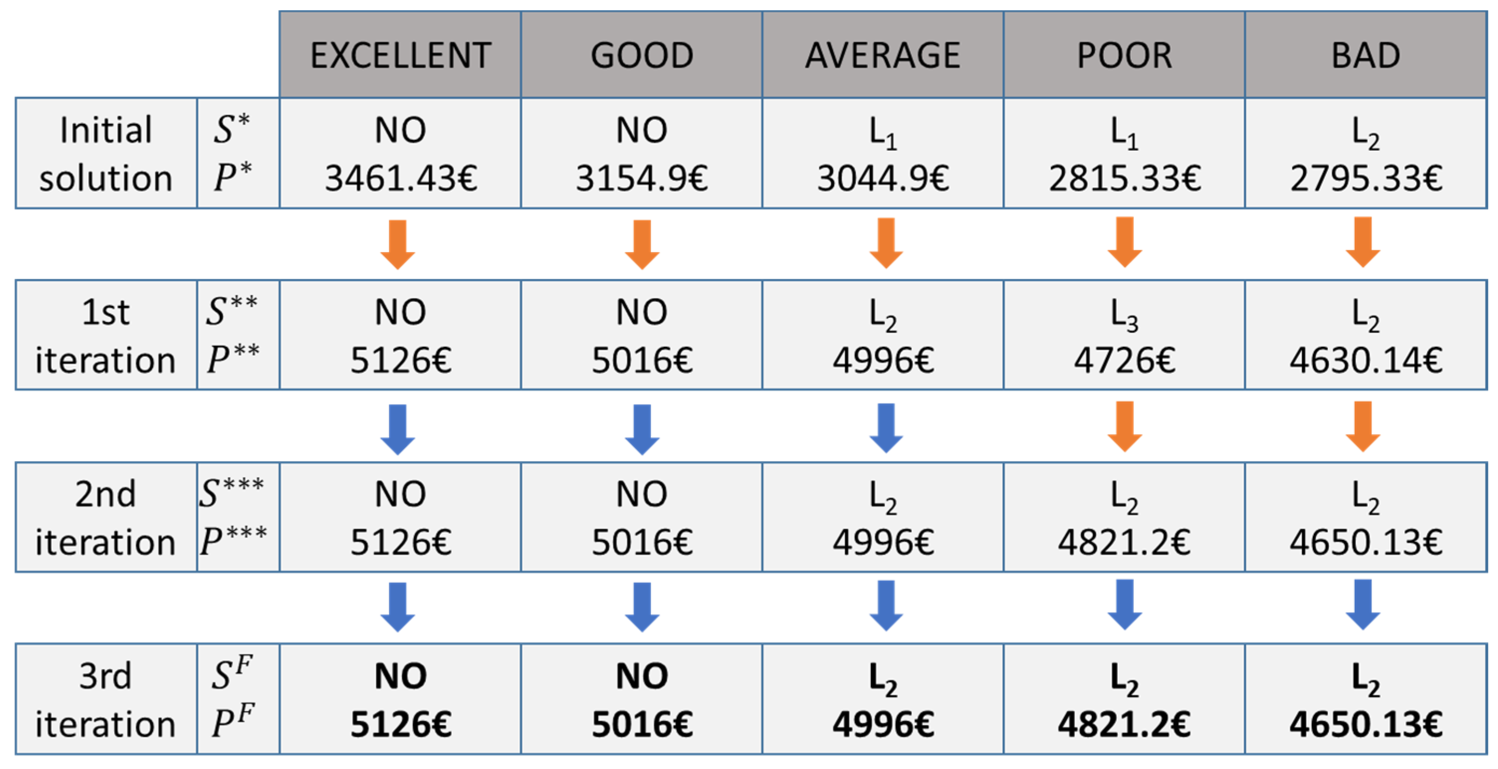
The improvement of the maintenance policy and the resultant discounted profit of the manufacturing system is shown in Figure 8.

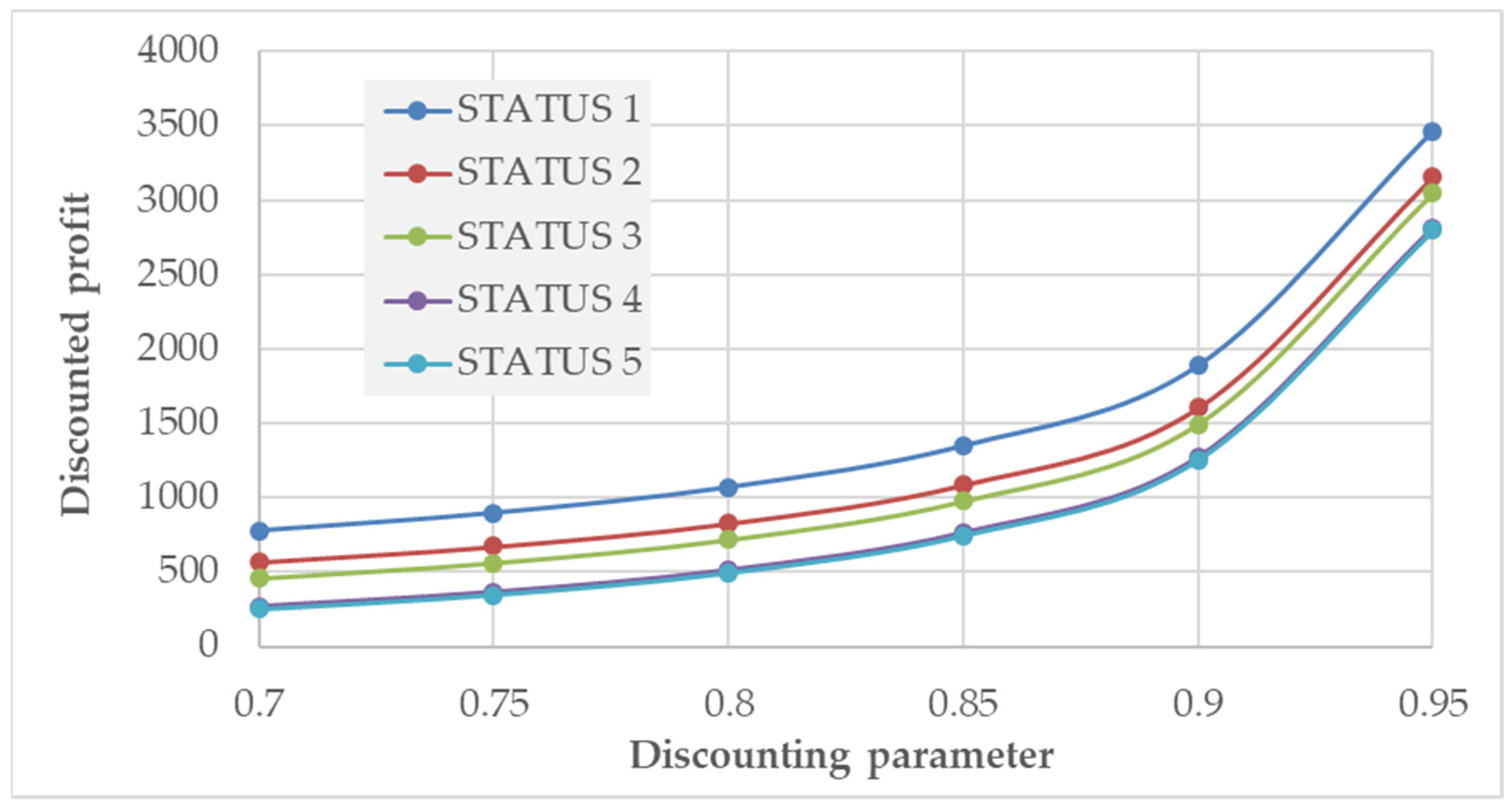
The discounted profit resulting from the optimized maintenance policy is influenced by the parameters of the physical systems and the cost model. Figure 9 and

Table A3. Impact of the discounting parameter on the discounted profit resulting from the optimized maintenance policy in the case of different initial status of the system (best status is Status 1 and worst status is Status 5).

	$\mathit{\vartheta }=0.7$	$\mathit{\vartheta }=0.75$	$\mathit{\vartheta }=0.8$	$\mathit{\vartheta }=0.85$	$\mathit{\vartheta }=0.9$	$\mathit{\vartheta }=0.95$
Status 1	778.03	896.78	1069.19	1346.84	1885.68	3461.42
Status 2	567.70	671.60	827.19	1086.19	1603.65	3154.91
Status 3	457.71	561.60	717.19	976.19	1493.65	3044.89
Status 4	269.46	365.59	513.20	763.94	1272.87	2815.33
Status 5	249.46	345.61	493.20	743.94	1252.87	2795.33

demonstrate the influence of discounting parameter $\vartheta$ on the discounted profit. As Figure 9 shows, the increased value of the discount parameter leads to an increase in discounted profit.

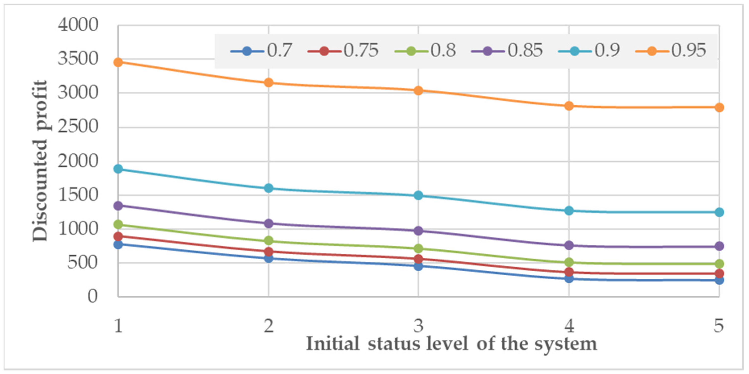
The discounted profit depends on the initial status level of the system. Figure 10 demonstrates the influence of initial status level of the system on the discounted profit. As Figure 10 shows, the better status level causes higher discounted profit and the increased $\vartheta$ value also increases the discounted profit for all initial system statuses.

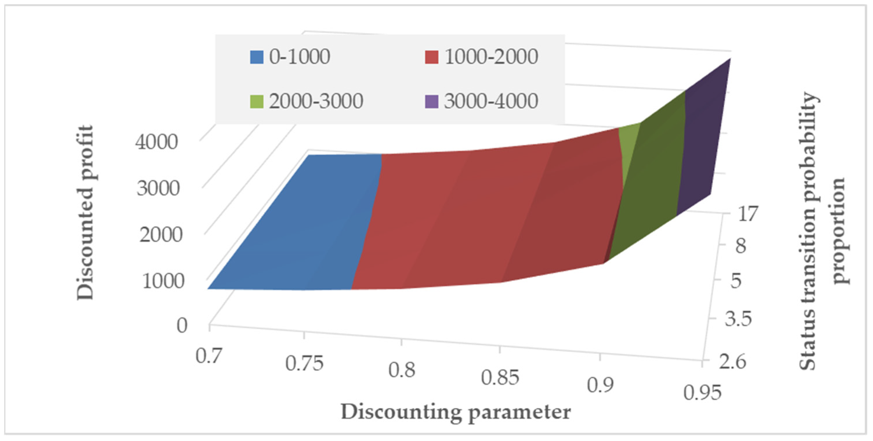
The impact of the initial system status and the $\vartheta$ discount parameter on the discounted profit is shown in Figure 11 and

Table A4. Impact of the initial system status and the $\vartheta$ discount parameter on the discounted profit resulted by the optimized maintenance policy.

	$\frac{{\mathit{\gamma }}_{\mathit{E}\to \mathit{E}}}{{\mathit{\gamma }}_{\mathit{G}\to \mathit{E}}}=2.6$	$\frac{{\mathit{\gamma }}_{\mathit{E}\to \mathit{E}}}{{\mathit{\gamma }}_{\mathit{G}\to \mathit{E}}}=3.5$	$\frac{{\mathit{\gamma }}_{\mathit{E}\to \mathit{E}}}{{\mathit{\gamma }}_{\mathit{G}\to \mathit{E}}}=5.0$	$\frac{{\mathit{\gamma }}_{\mathit{E}\to \mathit{E}}}{{\mathit{\gamma }}_{\mathit{G}\to \mathit{E}}}=8.0$	$\frac{{\mathit{\gamma }}_{\mathit{E}\to \mathit{E}}}{{\mathit{\gamma }}_{\mathit{G}\to \mathit{E}}}=17.0$
$\vartheta =0.7$	791.53	806.90	824.53	844.95	868.91
$\vartheta =0.75$	913.25	932.34	954.69	981.23	1013.26
$\vartheta =0.8$	1089.20	1113.02	1141.60	1176.53	1220.2
$\vartheta =0.85$	1371.60	1401.54	1438.53	1485.32	1546.45
$\vartheta =0.9$	1916.27	1954.28	2002.84	2066.99	2155.71
$\vartheta =0.95$	3499.49	3548.35	3613.36	3704.09	3839.60

. The sensitivity analysis shows that optimal maintenance policy is influenced by the parameters of the technological system and the corresponding cost model represented by the $\vartheta$ discount parameter.

The discount parameter does not influence the optimal maintenance policy, but it has a great impact on the discounted profit, because energy costs have to be taken into consideration as discounted costs. The above-described scenario validates the digital twin-based maintenance policy optimization and justifies the maintenance policy in both conventional and cyber-physical manufacturing systems. Services must be optimized in order to increase performance and ensure that all technological and logistics resources can operate at 100% efficiency at all times. To summarize, the proposed Howard’s policy iteration technique-based optimization model makes it possible to analyze the impact of maintenance policy on the performance parameters of technological and logistics processes and decrease the energy consumption and the related discounted costs.

As the findings of the literature review show, the articles that addressed the maintenance policy optimization are focusing on conventional production environments, but none of the articles aimed to identify the potential in a cyber-physical production environment, where Industry 4.0 technologies can increase the impact of the maintenance policy optimization. The comparison of our results with those from other studies shows that the optimization of maintenance policies in cyber-physical environments still requires more attention and research.

5. Discussion and Conclusions

Supply chain optimization is a key factor for a sustainable, cost-efficient economy [70]. The maintenance of production and service processes represent an important part of value chains; maintenance is important not only in the field of manufacturing, but also in the processes of purchasing and distribution. The fourth industrial revolution indicates new directions for the improvement of maintenance processes and their policies. Maintenance policies are discussed in a wide range of literature, but only a few of them focus on the potentials of linking energy and maintenance using real-time data for discrete event simulation. The content analysis part of the literature review showed that existing works mainly discuss the energy efficiency of the primary processes, and that the energy aspects of maintenance processes are out of their scope. To try to fill this gap, this analysis has developed a maintenance policy optimization methodology to analyze an existing maintenance policy based on value determination equations and improve them based on Howard’s policy iteration technique. In the model, a wide range of objective functions can be defined, such as costs, reliability, availability, sustainability, or GHG emission, while different constraints can also be taken into consideration. The described methodology shows that the optimization of maintenance policy has a great impact on energy consumption, GHG emission, and profit of the manufacturing system, and that it can support the optimization of maintenance policy, because real-time data collection can improve the efficiency of failure data forecasting and status information collection.

As a managerial impact, I would like to mention that the above-described methodology can support managerial decisions regarding organizational, technological, and logistical aspects of maintenance strategies. As the computational results show, the maintenance policy influences the energy consumption of both the manufacturing processes and the maintenance operations, therefore strategic decisions regarding maintenance policy have a great impact on the costs and income of the whole system. The electricity generation source of the energy used in production and maintenance has a great impact on the GHG emissions, making it important to find the best suitable maintenance strategy for manufacturing systems, and this is also an important managerial impact of the proposed approach.

If real data is available from an industrial application, then through data mining techniques and digital twin-based simulation this model can be extended again for further study regarding the effect of real-time optimization in a sustainable manufacturing system. As in the case of this proposed model, a wide range of energy- and emission-related constraints can immediately be incorporated within the model, and heuristics or metaheuristics can be applied for optimization, which is another immediate extension of the problem [71]. The conclusions and research implications can be summarized as follows:

• The development of new maintenance policy optimization methods must include Industry 4.0 technologies to improve the performance and reliability of algorithms and techniques. A new maintenance policy optimization method was developed for the improvement of available maintenance policies to improve the discounted profit of the manufacturing system, while energy efficiency and GHG emissions reduction are taken into consideration. The computational results of the analyzed scenario show, that the maintenance policy has a great impact on the cost reduction. In the demonstrated case, cost reduction of 38% was calculated, taking natural gas as the electricity generation source. The energy consumption cost was calculated on the basis of the levelized cost of the electricity.
• The design and operation of maintenance processes in services and production systems is a great challenge for researchers, because the complex and stochastic environment can lead to complex optimization problems.
• The computational results validated the described mathematical model and the Howard’s policy iteration-based optimization algorithm. The integration of value determination equations and Howard’s policy iteration-based optimization with energy-consumption and GHG emission minimization is a suitable tool to reduce costs from a maintenance policy point of view. As the computational results show, the different electricity generation sources influence the virtual GHG emission, which is virtual from the manufacturing system’s point of view, as the real emissions are generated at the electricity generation plant and not at the manufacturing plant.

In the case of NP-hard problems, heuristic and metaheuristic algorithms can solve the optimization problems [72]. A further study of the proposed work would be the integration of the above-mentioned methodology with a real-time heuristic policy optimization. Digital twin-based discrete event simulation makes it possible to analyze data from smart sensors of the manufacturing system and link the results of analysis to the optimization process to find the best maintenance policy for the current status of the resources in the manufacturing system.

In the case of a multi-level optimization, the described methodology can be improved and the new algorithm could have the following main phases: (a) data collection from the physical system and transformation of data to the digital twin; (b) definition of objective functions and constraints of the maintenance strategy; (c) long-term optimization of the maintenance policy based on Howard’s policy iteration method and value determination equations, including the costs of energy consumption and GHG emission calculation based on the levelized cost of energy and electricity generation sources; (d) collection of real-time failure data and status information from the digital twin; (e) analysis of the maintenance policy based on value determination equations; (f) real-time heuristic optimization of the long-term maintenance policy (re-optimization or correction based on real-time failure data and status information) from a cost, energy consumption, and GHG emissions perspective. This new, multi-level optimization process can be discussed within the frame of further study (see future plans in Figure A3). Taking into consideration the maturity of Industry 4.0 technologies [73], another future research direction is the integration of other I4.0 technologies (RFID, RTLS) with maintenance processes [74].

References

1. Telek, P.; Bányai, T. Complex design of integrated material flow systems. Adv. Logist. Syst. Theory Pract. 2013, 7, 105–110. [Google Scholar]
2. Andre, L. 35 Latest Maintenance Statistics for 2021: Data, Adoption & Strategies. Available online: https://financesonline.com/maintenance-statistics/ (accessed on 22 July 2021).
3. Savolainen, J.; Urbani, M. Maintenance optimization for a multi-unit system with digital twin simulation. J. Intell. Manuf. 2021, 32, 1953–1973. [Google Scholar] [CrossRef]
4. Bevilacqua, M.; Bottani, E.; Ciarapica, F.E.; Costantino, F.; Di Donato, L.; Ferraro, A.; Mazzuto, G.; Monteriù, A.; Nardini, G.; Ortenzi, M.; et al. Digital Twin Reference Model Development to Prevent Operators’ Risk in Process Plants. Sustainability 2020, 12, 1088. [Google Scholar] [CrossRef] [Green Version]
5. Bhuniya, S.; Pareek, S.; Sarkar, B.; Sett, B.K. A Smart Production Process for the Optimum Energy Consumption with Maintenance Policy under a Supply Chain Management. Processes 2021, 9, 19. [Google Scholar] [CrossRef]
6. Khanna, A.; Gautam, P.; Sarkar, B.; Jaggi, C.K. Integrated vendor–buyer strategies for imperfect production systems with maintenance and warranty policy. RAIRO-Oper. Res. 2020, 54, 435–450. [Google Scholar] [CrossRef] [Green Version]
7. Sett, B.K.; Sarkar, S.; Sarkar, B. Optimal buffer inventory and inspection errors in an imperfect production system with preventive maintenance. Int. J. Adv. Manuf. Technol. 2017, 90, 545–560. [Google Scholar] [CrossRef]
8. Aznia, A.H.; Ahmad, R.; Noh, Z.A.M.; Hazwani, F.; Hayaati, N. Systematic Review for Network Survivability Analysis in MANETS. Procedia-Soc. Behav. Sci. 2015, 195, 1872–1881. [Google Scholar] [CrossRef] [Green Version]
9. Menipaz, E. Optimization of stochastic maintenance policies. Eur. J. Oper. Res. 1978, 2, 97–106. [Google Scholar] [CrossRef]
10. Vaurio, J.K. On time-dependent availability and maintenance optimization of standby units under various maintenance policies. Reliab. Eng. Syst. Saf. 1997, 56, 79–89. [Google Scholar] [CrossRef]
11. Ye, Y.; Grossmann, I.E.; Pinto, J.M.; Ramaswamy, S. Integrated optimization of design, storage sizing, and maintenance policy as a Markov decision process considering varying failure rates. Comput. Chem. Eng. 2020, 142, 107052. [Google Scholar] [CrossRef]
12. Xiang, Y. Joint optimization of X¯ control chart and preventive maintenance policies: A discrete-time Markov chain approach. Eur. J. Oper. Res. 2013, 229, 382–390. [Google Scholar] [CrossRef]
13. Fauriat, W.; Zio, E. Optimization of an aperiodic sequential inspection and condition-based maintenance policy driven by value of information. Reliab. Eng. Syst. Saf. 2020, 204, 107133. [Google Scholar] [CrossRef]
14. Lesage, A.; Dehombreux, P. Maintenance & Quality Control: A First Methodological Approach for Maintenance Policy Optimization. IFAC Proc. Vol. 2012, 45, 1041–1046. [Google Scholar] [CrossRef]
15. Sarker, R.; Haque, A. Optimization of maintenance and spare provisioning policy using simulation. Appl. Math. Model. 2000, 24, 751–760. [Google Scholar] [CrossRef]
16. Li, Z.; Zhong, S.; Lin, L. An aero-engine life-cycle maintenance policy optimization algorithm: Reinforcement learning approach. Chin. J. Aeronaut. 2019, 32, 2133–2150. [Google Scholar] [CrossRef]
17. Samrout, M.; Châtelet, E.; Kouta, R.; Chebbo, N. Optimization of maintenance policy using the proportional hazard model. Reliab. Eng. Syst. Saf. 2009, 94, 44–52. [Google Scholar] [CrossRef]
18. Panagiotidou, S. Joint optimization of spare parts ordering and maintenance policies for multiple identical items subject to silent failures. Eur. J. Oper. Res. 2013, 235, 300–314. [Google Scholar] [CrossRef]
19. Zied, H.; Sofiene, D.; Nidhal, R. Production/Maintenance policies optimization with operational age concept in a subcontracting constraint. IFAC Proc. Vol. 2011, 44, 5213–5218. [Google Scholar] [CrossRef]
20. Coria, V.H.; Maximov, S.; Rivas-Dávalos, F.; Melchor, C.L.; Guardado, J.L. Analytical method for optimization of maintenance policy based on available system failure data. Reliab. Eng. Syst. Saf. 2015, 135, 55–63. [Google Scholar] [CrossRef]
21. Zahedi-Hosseini, F.; Scarf, P.; Syntetos, A. Joint optimisation of inspection maintenance and spare parts provisioning: A comparative study of inventory policies using simulation and survey data. Reliab. Eng. Syst. Saf. 2017, 168, 306–316. [Google Scholar] [CrossRef]
22. Wu, S.; Chen, Y.; Wu, Q.; Wang, Z. Linking component importance to optimisation of preventive maintenance policy. Reliab. Eng. Syst. Saf. 2016, 146, 26–32. [Google Scholar] [CrossRef] [Green Version]
23. Gao, K.; Peng, R.; Qu, L.; Wu, S. Jointly optimizing lot sizing and maintenance policy for a production system with two failure modes. Reliab. Eng. Syst. Saf. 2020, 202, 106996. [Google Scholar] [CrossRef]
24. Gao, W.; Yang, T.; Chen, L.; Wu, S. Joint optimisation on maintenance policy and resources for multi-unit parallel production system. Comput. Ind. Eng. 2021, 159, 107491. [Google Scholar] [CrossRef]
25. Manzoor, F.; Wei, L.; Bányai, T.; Nurunnabi, M.; Subhan, Q.A. An Examination of Sustainable HRM Practices on Job Performance: An Application of Training as a Moderator. Sustainability 2019, 11, 2263. [Google Scholar] [CrossRef] [Green Version]
26. Emami-Mehrgani, B.; Neumann, W.P.; Nadeau, S.; Bazrafshan, M. Considering human error in optimizing production and corrective and preventive maintenance policies for manufacturing systems. Appl. Math. Model. 2016, 40, 2056–2074. [Google Scholar] [CrossRef]
27. Zhang, X.; Zeng, J. Joint optimization of condition-based opportunistic maintenance and spare parts provisioning policy in multiunit systems. Eur. J. Oper. Res. 2017, 262, 479–498. [Google Scholar] [CrossRef]
28. Golbasi, O.; Turan, M.O. A discrete-event simulation algorithm for the optimization of multi-scenario maintenance policies. Comput. Ind. Eng. 2020, 145, 106514. [Google Scholar] [CrossRef]
29. Boudhar, H.; Dahane, M.; Rezg, N. Joint optimisation of spare parts demand and remanufacturing policy under condition-based maintenance for stochastic deteriorating manufacturing system. IFAC Proc. Vol. 2013, 46, 414–419. [Google Scholar] [CrossRef]
30. Wang, J.; Zhao, X.; Guo, X. Optimizing wind turbine’s maintenance policies under performance-based contract. Renew. Energy 2019, 135, 626–634. [Google Scholar] [CrossRef]
31. Regattieri, A.; Giazzi, A.; Gamberi, M.; Gamberini, R. An innovative method to optimize the maintenance policies in an aircraft: General framework and case study. J. Air Transp. Manag. 2015, 44–45, 8–20. [Google Scholar] [CrossRef]
32. Park, M.; Jung, K.M.; Park, D.H. Optimization of periodic preventive maintenance policy following the expiration of two-dimensional warranty. Reliab. Eng. Syst. Saf. 2018, 170, 1–9. [Google Scholar] [CrossRef]
33. Delanka-Pedige, H.M.K.; Munasinghe-Arachchige, S.P.; Abeysiriwardana-Arachchige, I.S.A.; Nirmalakhandan, N. Evaluating wastewater treatment infrastructure systems based on UN Sustainable Development Goals and targets. J. Clean. Prod. 2021, 298, 126795. [Google Scholar] [CrossRef]
34. Guerrini, A.; Romano, G.; Ferretti, S.; Fibbi, D.; Daddi, D. A Performance Measurement Tool Leading Wastewater Treatment Plants toward Economic Efficiency and Sustainability. Sustainability 2016, 8, 1250. [Google Scholar] [CrossRef] [Green Version]
35. Gu, Y.; Li, Y.; Li, X.; Luo, P.; Wang, H.; Robinson, Z.P.; Wang, X.; Wu, J.; Li, F. The feasibility and challenges of energy self-sufficient wastewater treatment plants. Appl. Energy 2017, 204, 1463–1475. [Google Scholar] [CrossRef] [Green Version]
36. Díaz-Madroñero Boluda, F.M.; Pérez-Sánchez, M.; Satorre-Aznar, J.R.; Mula, J.; López Jiménez, P.A. Analysis of a wastewater treatment plant using fuzzy goal programming as a management tool: A case study. J. Clean. Prod. 2018, 180, 20–33. [Google Scholar] [CrossRef]
37. Munasinghe-Arachchige, S.P.; Abeysiriwardana-Arachchige, I.S.A.; Delanka-Pedige, H.M.K.; Nirmalakhandan, N. Sewage treatment process refinement and intensification using multi-criteria decision making approach: A case study. J. Water Process. Eng. 2020, 37, 101485. [Google Scholar] [CrossRef]
38. Li, Z.; Zi, Y.; Chen, J.; Pan, J.; Zhou, Z. Performance-guided maintenance policy and optimization for transmission system of shipborne antenna with multiple components. Ocean. Eng. 2020, 199, 106903. [Google Scholar] [CrossRef]
39. Gómez, A.; Carnero, M.C. Decision Support System for maintenance policy optimization in medicinal gases subsystems. IFAC-PapersOnLine 2016, 49, 268–273. [Google Scholar] [CrossRef]
40. Caputo, A.C.; Pelagagge, P.M.; Salini, P. Joint economic optimization of heat exchanger design and maintenance policy. Appl. Therm. Eng. 2011, 31, 1381–1392. [Google Scholar] [CrossRef] [Green Version]
41. Nourelfath, M.; Ait-Kadi, D. Optimization of series–parallel multi-state systems under maintenance policies. Reliab. Eng. Syst. Saf. 2007, 92, 1620–1626. [Google Scholar] [CrossRef]
42. Marseguerra, M.; Zio, E. Optimizing maintenance and repair policies via a combination of genetic algorithms and Monte Carlo simulation. Reliab. Eng. Syst. Saf. 2000, 68, 69–83. [Google Scholar] [CrossRef]
43. Melchor-Hernández, C.L.; Rivas-Dávalos, F.; Maximov, S.; Coria, V.H.; Guardado, J.L. A model for optimizing maintenance policy for power equipment. Int. J. Electr. Power Energy Syst. 2015, 68, 304–312. [Google Scholar] [CrossRef]
44. Martinod, R.M.; Bistorin, O.; Castañeda, L.F.; Rezg, N. Maintenance policy optimisation for multi-component systems considering degradation of components and imperfect maintenance actions. Comput. Ind. Eng. 2018, 124, 100–112. [Google Scholar] [CrossRef] [Green Version]
45. Jiang, Y.; Chen, M.; Zhou, D. Joint optimization of preventive maintenance and inventory policies for multi-unit systems subject to deteriorating spare part inventory. J. Manuf. Syst. 2015, 35, 191–205. [Google Scholar] [CrossRef]
46. Ajah, A.N.; Grievink, J.; Herder, P.; Weijnen, M. Adaptive control approach in modeling life-cycle maintenance policy selection and optimisation during infrastructure systems conceptual design & operation. Comput. Aided Chem. Eng. 2007, 24, 1145–1150. [Google Scholar] [CrossRef]
47. Bányai, Á.; Illés, B.; Glistau, E.; Machado, N.I.C.; Tamás, P.; Manzoor, F.; Bányai, T. Smart cyber-physical manufacturing: Extended and real-time optimization of logistics resources in matrix production. Appl. Sci. 2019, 9, 1287. [Google Scholar] [CrossRef] [Green Version]
48. Dedopoulos, I.T.; Shah, N. Preventive maintenance policy optimization for multipurpose plant equipment. Comput. Chem. Eng. 1995, 19, 693–698. [Google Scholar] [CrossRef]
49. Xia, T.B.; Shi, G.; Si, G.J.; Du, S.C.; Xi, L.F. Energy-oriented joint optimization of machine maintenance and tool replacement in sustainable manufacturing. J. Manuf. Syst. 2021, 59, 261–271. [Google Scholar] [CrossRef]
50. Xu, W.G.; Cao, L. Optimal maintenance control of machine tools for energy efficient manufacturing. Int. J. Adv. Manuf. Technol. 2019, 104, 3303–3311. [Google Scholar] [CrossRef]
51. Zhou, B.H.; Yi, Q. An energy-oriented maintenance policy under energy and quality constraints for a multielement-dependent degradation batch production system. J. Manuf. Syst. 2021, 59, 631–645. [Google Scholar] [CrossRef]
52. Keramati, A.; Lu, P.; Sobhani, A.; Esmaeili, S.A.H. Impact of Forest Road Maintenance Policies on Log Transportation Cost, Routing, and Carbon-Emission Trade-Offs: Oregon Case Study. J. Transp. Eng. Part A-Syst. 2020, 146, 04020028. [Google Scholar] [CrossRef]
53. Drent, C.; Kapodistria, S.; Resing, J.A.C. Condition-based maintenance policies under imperfect maintenance at scheduled and unscheduled opportunities. Queueing Syst. 2019, 93, 269–308. [Google Scholar] [CrossRef] [Green Version]
54. Yu, T.; Zhu, C.; Chang, Q.; Wang, J.F. Imperfect corrective maintenance scheduling for energy efficient manufacturing systems through online task allocation method. J. Manuf. Syst. 2019, 53, 282–290. [Google Scholar] [CrossRef]
55. Seyr, H.; Muskulus, M. Use of Markov Decision Processes in the Evaluation of Corrective Maintenance Scheduling Policies for Offshore Wind Farms. Energies 2019, 12, 2993. [Google Scholar] [CrossRef] [Green Version]
56. Erguido, A.; Marquez, A.C.; Castellano, E.; Fernandez, J.F.G. A dynamic opportunistic maintenance model to maximize energy-based availability while reducing the life cycle cost of wind farms. Renew. Energy 2017, 114, 843–856. [Google Scholar] [CrossRef] [Green Version]
57. Hajej, Z.; Nidhal, R.; Anis, C.; Bouzoubaa, M. An optimal integrated production and maintenance strategy for a multi-wind turbines system. Int. J. Prod. Res. 2020, 58, 6417–6440. [Google Scholar] [CrossRef]
58. Pradhan, P.; Kishore, S.; Defourny, B. Optimal Predictive Maintenance Policy for an Ocean Wave Farm. IEEE Trans. Sustain. Energy 2019, 10, 1993–2004. [Google Scholar] [CrossRef]
59. Do, P.; Hoang, A.; Iung, B.; Vu, H.C. Energy efficiency for condition-based maintenance decision-making: Application to a manufacturing platform. Proc. Inst. Mech. Eng. Part O-J. Risk Reliab. 2018, 232, 379–388. [Google Scholar] [CrossRef]
60. Jiang, A.P.; Dong, N.; Tam, K.L.; Lyu, C.H. Development and Optimization of a Condition-Based Maintenance Policy with Sustainability Requirements for Production System. Math. Probl. Eng. 2018, 2018, 4187575. [Google Scholar] [CrossRef]
61. Jiang, A.P.; Wang, Y.Y.; Cheng, Y.D. A Condition-Based Opportunistic Maintenance Policy Integrated with Energy Efficiency for Two-Component Parallel Systems. J. Ind. Eng. Manag.-JIEM 2018, 11, 749–768. [Google Scholar] [CrossRef]
62. Xia, T.B.; Xi, L.F.; Du, S.C.; Xiao, L.; Pan, E.S. Energy-Oriented Maintenance Decision-Making for Sustainable Manufacturing Based on Energy Saving Window. J. Manuf. Sci. Eng.-Trans. ASME 2018, 140, 051001. [Google Scholar] [CrossRef]
63. Demichela, M.; Baldissone, G.; Darabnia, B. Using Field Data for Energy Efficiency Based on Maintenance and Operational Optimisation. A Step towards PHM in Process Plants. Processes 2018, 6, 25. [Google Scholar] [CrossRef] [Green Version]
64. Zhou, W.H.; Zheng, Z.B.; Xie, W. A control-chart-based queueing approach for service facility maintenance with energy-delay tradeoff. Eur. J. Oper. Res. 2017, 261, 613–625. [Google Scholar] [CrossRef]
65. De Bernardini, L. Maintenance Management: MES or ERP? Available online: https://www.automationworld.com/products/software/blog/13312746/maintenance-management-mes-or-erp (accessed on 20 July 2021).
66. Firdaus, N.; Samat, H.A.; Mohamad, N. Maintenance for energy efficiency: A review. IOP Conf. Ser. Mater. Sci. Eng. 2019, 530, 012047. [Google Scholar] [CrossRef]
67. Winston, W.L. Operations Research: Applications and Algorithms; Thomson Brooks Cole: Victoria, Australia, 2004. [Google Scholar]
68. International Renewable Energy Agency. Renewable Power Generation Costs in 2020. Available online: https://www.irena.org/publications (accessed on 16 August 2021).
69. World Nuclear Association. Comparison of Lifecycle Greenhouse Gas Emissions of Various Electricity Generation Sources; World Nuclear Association: London, UK, 2011; pp. 1–12. [Google Scholar]
70. Bányai, T. Supply chain optimization of outsourced blending technologies. J. Appl. Econ. Sci. 2017, 12, 960–976. [Google Scholar]
71. Sarkar, M.; Kim, S.; Jemai, J.; Ganguly, B.; Sarkar, B. An Application of Time-Dependent Holding Costs and System Reliability in a Multi-Item Sustainable Economic Energy Efficient Reliable Manufacturing System. Energies 2019, 12, 2857. [Google Scholar] [CrossRef] [Green Version]
72. Veres, P.; Bányai, T.; Illés, B. Optimization of in-plant production supply with black hole algorithm. Solid State Phenom. 2017, 261, 503–508. [Google Scholar] [CrossRef]
73. Fükő, L.; Illés, B.; Tamás, P.; Skapinyecz, R.; Cservenák, Á. Methods for determining maturity evaluation system in industry 4.0. Rezan. Instrum. Tekhnologicheskih Sist. 2020, 93, 9–14. [Google Scholar] [CrossRef]
74. Tamás, P.; Bátori, T. Application possibilities of RTLS system in production logistics. J. Prod. Eng. 2021, 24, 22–28. [Google Scholar] [CrossRef]
Figure 1. Summary of background assumptions from the linkage of maintenance and energy point of view.
Energies 14 05674 g001
Figure 2. Methodological process of the systematic literature review based on searching in Science Direct.
Energies 14 05674 g002
Figure 3. Classification of articles by subject areas based on search in Science Direct.
Energies 14 05674 g003
Figure 4. Methodological framework of maintenance policy optimization research based on the content analysis part of the systematic literature review.
Energies 14 05674 g004
Figure 5. Model framework of digital twin-supported maintenance policy optimization.
Energies 14 05674 g005
Figure 6. Multi-level maintenance policy optimization based on Howard’s policy iteration.
Energies 14 05674 g006
Figure 7. Levelized cost of energy depending on the electricity generation source in USD/kWh [68].
Energies 14 05674 g007
Figure 8. Computational results of maintenance strategy optimization based on Howard’s Policy Iteration Method (orange arrows: changing strategy, increased profit, decreased energy consumption, and decreased virtual GHG emission; blue arrows: unchanged strategy, profit, energy consumptions, and GHG emission).
Energies 14 05674 g008
Figure 9. Impact of the discounting parameter on the discounted energy-consumption-based profit resulting from the optimized maintenance policy in the case of different initial status of the system (best status is Status 1 and worst status is Status 5).
Energies 14 05674 g009
Figure 10. Impact of the initial system status on the discounted energy-consumption-based profit resulting from the optimized maintenance policy in the case of different discount parameters.
Energies 14 05674 g010
Figure 11. Impact of the initial system status and the ϑ discount parameter on the discounted profit resulted by the optimized maintenance policy.
Energies 14 05674 g011