
A Simulation Environment for Training a Reinforcement Learning Agent Trading a Battery Storage


Abstract
:1. Introduction
2. Literature Review
2.1. Batteries in Primary Frequency Reserves
2.2. Reinforcement Learning Applications for Batteries
- •
- Real-time control.
- •
- Medium-term decision-making for optimizing some operational criteria such as electricity costs or photovoltaic self-consumption. In many cases, this involves decision-making once per electricity market interval, which in many cases is hourly.
- •
- Long-term studies to support investment decisions.
3. Battery Trading System
4. Implementation
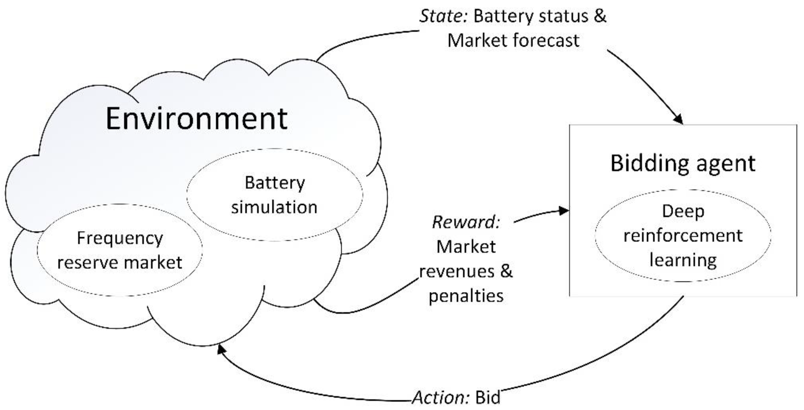
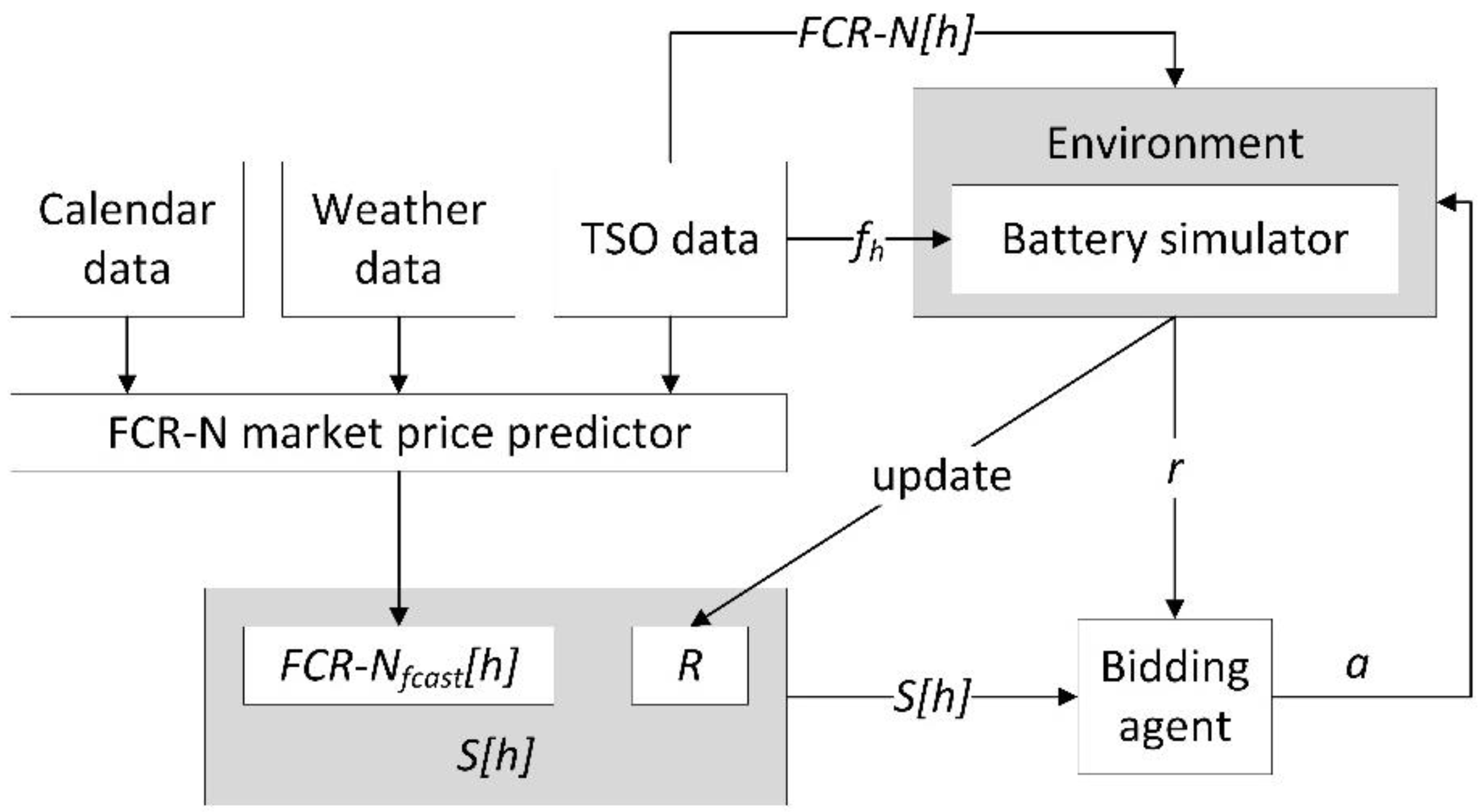
4.1. Enviroment
4.2. Bidding Agent
5. Result
6. Conclusions
Author Contributions
Funding
Institutional Review Board Statement
Informed Consent Statement
Data Availability Statement
Acknowledgments
Conflicts of Interest
References
- Peters, I.M.; Breyer, C.; Jaffer, S.A.; Kurtz, S.; Reindl, T.; Sinton, R.; Vetter, M. The role of batteries in meeting the PV terawatt challenge. Joule 2021, 5, 1353–1370. [Google Scholar] [CrossRef]
- de Siqueira Silva, L.M.; Peng, W. Control strategy to smooth wind power output using battery energy storage system: A review. J. Energy Storage 2021, 35, 102252. [Google Scholar] [CrossRef]
- Sepúlveda-Mora, S.B.; Hegedus, S. Making the case for time-of-use electric rates to boost the value of battery storage in commercial buildings with grid connected PV systems. Energy 2021, 218, 119447. [Google Scholar] [CrossRef]
- Loukatou, A.; Johnson, P.; Howell, S.; Duck, P. Optimal valuation of wind energy projects co-located with battery storage. Appl. Energy 2021, 283, 116247. [Google Scholar] [CrossRef]
- Akagi, S.; Yoshizawa, S.; Ito, M.; Fujimoto, Y.; Miyazaki, T.; Hayashi, Y.; Tawa, K.; Hisada, T.; Yano, T. Multipurpose control and planning method for battery energy storage systems in distribution network with photovoltaic plant. Int. J. Electr. Power Energy Syst. 2020, 116, 105485. [Google Scholar] [CrossRef]
- Nefedov, E.; Sierla, S.; Vyatkin, V. Internet of energy approach for sustainable use of electric vehicles as energy storage of prosumer buildings. Energies 2018, 11, 2165. [Google Scholar] [CrossRef] [Green Version]
- Ge, X.; Ahmed, F.W.; Rezvani, A.; Aljojo, N.; Samad, S.; Foong, L.K. Implementation of a novel hybrid BAT-Fuzzy controller based MPPT for grid-connected PV-battery system. Control. Eng. Pract. 2020, 98, 104380. [Google Scholar] [CrossRef]
- Aldosary, A.; Ali, Z.M.; Alhaider, M.M.; Ghahremani, M.; Dadfar, S.; Suzuki, K. A modified shuffled frog algorithm to improve MPPT controller in PV System with storage batteries under variable atmospheric conditions. Control. Eng. Pract. 2021, 112, 104831. [Google Scholar] [CrossRef]
- Ciupageanu, D.; Barelli, L.; Lazaroiu, G. Real-time stochastic power management strategies in hybrid renewable energy systems: A review of key applications and perspectives. Electr. Power Syst. Res. 2020, 187, 106497. [Google Scholar] [CrossRef]
- Lin, L.; Jia, Y.; Ma, M.; Jin, X.; Zhu, L.; Luo, H. Long-term stable operation control method of dual-battery energy storage system for smoothing wind power fluctuations. Int. J. Electr. Power Energy Syst. 2021, 129, 106878. [Google Scholar] [CrossRef]
- Ryu, A.; Ishii, H.; Hayashi, Y. Battery smoothing control for photovoltaic system using short-term forecast with total sky images. Electr. Power Syst. Res. 2021, 190, 106645. [Google Scholar] [CrossRef]
- Subramanya, R.; Yli-Ojanperä, M.; Sierla, S.; Hölttä, T.; Valtakari, J.; Vyatkin, V. A virtual power plant solution for aggregating photovoltaic systems and other distributed energy resources for northern european primary frequency reserves. Energies 2021, 14, 1242. [Google Scholar] [CrossRef]
- Koller, M.; Borsche, T.; Ulbig, A.; Andersson, G. Review of grid applications with the Zurich 1MW battery energy storage system. Electr. Power Syst. Res. 2015, 120, 128–135. [Google Scholar] [CrossRef]
- Giovanelli, C.; Sierla, S.; Ichise, R.; Vyatkin, V. Exploiting artificial neural networks for the prediction of ancillary energy market prices. Energies 2018, 11, 1906. [Google Scholar] [CrossRef] [Green Version]
- Lund, H.; Hvelplund, F.; Østergaard, P.A.; Möller, B.; Mathiesen, B.V.; Karnøe, P.; Andersen, A.N.; Morthorst, P.E.; Karlsson, K.; Münster, M.; et al. System and market integration of wind power in Denmark. Energy Strategy Rev. 2013, 1, 143–156. [Google Scholar] [CrossRef] [Green Version]
- Bialek, J. What does the GB power outage on 9 August 2019 tell us about the current state of decarbonised power systems? Energy Policy 2020, 146, 111821. [Google Scholar] [CrossRef]
- Papadogiannis, K.A.; Hatziargyriou, N.D. Optimal allocation of primary reserve services in energy markets. IEEE Trans. Power Syst. 2004, 19, 652–659. [Google Scholar] [CrossRef]
- Pavić, I.; Capuder, T.; Kuzle, I. Low carbon technologies as providers of operational flexibility in future power systems. Appl. Energy 2016, 168, 724–738. [Google Scholar] [CrossRef]
- Zecchino, A.; Prostejovsky, A.M.; Ziras, C.; Marinelli, M. Large-scale provision of frequency control via V2G: The Bornholm power system case. Electr. Power Syst. Res. 2019, 170, 25–34. [Google Scholar] [CrossRef]
- Malik, A.; Ravishankar, J. A hybrid control approach for regulating frequency through demand response. Appl. Energy 2018, 210, 1347–1362. [Google Scholar] [CrossRef]
- Borsche, T.S.; de Santiago, J.; Andersson, G. Stochastic control of cooling appliances under disturbances for primary frequency reserves. Sustain. Energy Grids Netw. 2016, 7, 70–79. [Google Scholar] [CrossRef]
- Herre, L.; Tomasini, F.; Paridari, K.; Söder, L.; Nordström, L. Simplified model of integrated paper mill for optimal bidding in energy and reserve markets. Appl. Energy 2020, 279, 115857. [Google Scholar] [CrossRef]
- Ramírez, M.; Castellanos, R.; Calderón, G.; Malik, O. Placement and sizing of battery energy storage for primary frequency control in an isolated section of the Mexican power system. Electr. Power Syst. Res. 2018, 160, 142–150. [Google Scholar] [CrossRef]
- Killer, M.; Farrokhseresht, M.; Paterakis, N.G. Implementation of large-scale li-ion battery energy storage systems within the EMEA region. Appl. Energy 2020, 260, 114166. [Google Scholar] [CrossRef]
- Oudalov, A.; Chartouni, D.; Ohler, C. Optimizing a battery energy storage system for primary frequency control. IEEE Trans. Power Syst. 2007, 22, 1259–1266. [Google Scholar] [CrossRef]
- Andrenacci, N.; Pede, G.; Chiodo, E.; Lauria, D.; Mottola, F. Tools for life cycle estimation of energy storage system for primary frequency reserve. In Proceedings of the International Symposium on Power Electronics, Electrical Drives, Automation and Motion (SPEEDAM), Amalfi, Italy, 20–22 June 2018; pp. 1008–1013. [Google Scholar] [CrossRef]
- Karbouj, H.; Rather, Z.H.; Flynn, D.; Qazi, H.W. Non-synchronous fast frequency reserves in renewable energy integrated power systems: A critical review. Int. J. Electr. Power Energy Syst. 2019, 106, 488–501. [Google Scholar] [CrossRef]
- Srinivasan, L.; Markovic, U.; Vayá, M.G.; Hug, G. Provision of frequency control by a BESS in combination with flexible units. In Proceedings of the 5th IEEE International Energy Conference (ENERGYCON), Limassol, Cyprus, 3–7 June 2018; pp. 1–6. [Google Scholar] [CrossRef]
- Phan, B.C.; Lai, Y. Control strategy of a hybrid renewable energy system based on reinforcement learning approach for an isolated microgrid. Appl. Sci. 2019, 9, 4001. [Google Scholar] [CrossRef] [Green Version]
- Li, W.; Cui, H.; Nemeth, T.; Jansen, J.; Ünlübayir, C.; Wei, Z.; Zhang, L.; Wang, Z.; Ruan, J.; Dai, H.; et al. Deep reinforcement learning-based energy management of hybrid battery systems in electric vehicles. J. Energy Storage 2021, 36, 102355. [Google Scholar] [CrossRef]
- Chen, Z.; Hu, H.; Wu, Y.; Xiao, R.; Shen, J.; Liu, Y. Energy management for a power-split plug-in hybrid electric vehicle based on reinforcement learning. Appl. Sci. 2018, 8, 2494. [Google Scholar] [CrossRef] [Green Version]
- Sui, Y.; Song, S. A multi-agent reinforcement learning framework for lithium-ion battery scheduling problems. Energies 2020, 13, 1982. [Google Scholar] [CrossRef] [Green Version]
- Muriithi, G.; Chowdhury, S. Optimal energy management of a grid-tied solar pv-battery microgrid: A reinforcement learning approach. Energies 2021, 14, 2700. [Google Scholar] [CrossRef]
- Kim, S.; Lim, H. Reinforcement learning based energy management algorithm for smart energy buildings. Energies 2018, 11, 2010. [Google Scholar] [CrossRef] [Green Version]
- Lee, S.; Choi, D. Reinforcement learning-based energy management of smart home with rooftop solar photovoltaic system, energy storage system, and home appliances. Sensors 2019, 19, 3937. [Google Scholar] [CrossRef] [Green Version]
- Lee, S.; Choi, D. Energy management of smart home with home appliances, energy storage system and electric vehicle: A hierarchical deep reinforcement learning approach. Sensors 2020, 20, 2157. [Google Scholar] [CrossRef] [Green Version]
- Roesch, M.; Linder, C.; Zimmermann, R.; Rudolf, A.; Hohmann, A.; Reinhart, G. Smart grid for industry using multi-agent reinforcement learning. Appl. Sci. 2020, 10, 6900. [Google Scholar] [CrossRef]
- Kim, J.; Lee, B. Automatic P2P Energy trading model based on reinforcement learning using long short-term delayed reward. Energies 2020, 13, 5359. [Google Scholar] [CrossRef]
- Wang, N.; Xu, W.; Shao, W.; Xu, Z. A q-cube framework of reinforcement learning algorithm for continuous double auction among microgrids. Energies 2019, 12, 2891. [Google Scholar] [CrossRef] [Green Version]
- Mbuwir, B.V.; Ruelens, F.; Spiessens, F.; Deconinck, G. Battery energy management in a microgrid using batch reinforcement learning. Energies 2017, 10, 1846. [Google Scholar] [CrossRef] [Green Version]
- Zsembinszki, G.; Fernández, C.; Vérez, D.; Cabeza, L.F. Deep Learning optimal control for a complex hybrid energy storage system. Buildings 2021, 11, 194. [Google Scholar] [CrossRef]
- Lee, H.; Ji, D.; Cho, D. Optimal design of wireless charging electric bus system based on reinforcement learning. Energies 2019, 12, 1229. [Google Scholar] [CrossRef] [Green Version]
- Oh, E. Reinforcement-learning-based virtual energy storage system operation strategy for wind power forecast uncertainty management. Appl. Sci. 2020, 10, 6420. [Google Scholar] [CrossRef]
- Tsianikas, S.; Yousefi, N.; Zhou, J.; Rodgers, M.D.; Coit, D. A storage expansion planning framework using reinforcement learning and simulation-based optimization. Appl. Energy 2021, 290, 116778. [Google Scholar] [CrossRef]
- Sidorov, D.; Panasetsky, D.; Tomin, N.; Karamov, D.; Zhukov, A.; Muftahov, I.; Dreglea, A.; Liu, F.; Li, Y. Toward zero-emission hybrid AC/DC power systems with renewable energy sources and storages: A case study from Lake Baikal region. Energies 2020, 13, 1226. [Google Scholar] [CrossRef] [Green Version]
- Xu, B.; Shi, J.; Li, S.; Li, H.; Wang, Z. Energy consumption and battery aging minimization using a q-learning strategy for a battery/ultracapacitor electric vehicle. Energy 2021, 229, 120705. [Google Scholar] [CrossRef]
- Zhang, G.; Hu, W.; Cao, D.; Liu, W.; Huang, R.; Huang, Q.; Chen, Z.; Blaabjerg, F. Data-driven optimal energy management for a wind-solar-diesel-battery-reverse osmosis hybrid energy system using a deep reinforcement learning approach. Energy Convers. Manag. 2021, 227, 113608. [Google Scholar] [CrossRef]
- Fingrid. The Technical Requirements and the Prequalification Process of Frequency Containment Reserves (FCR). Available online: https://www.fingrid.fi/globalassets/dokumentit/en/electricity-market/reserves/appendix3---technical-requirements-and-prequalification-process-of-fcr.pdf (accessed on 6 July 2021).
- Fingrid. Fingridin reservikaupankäynti ja tiedonvaihto -ohje. Available online: https://www.fingrid.fi/globalassets/dokumentit/fi/sahkomarkkinat/reservit/fingridin-reservikaupankaynti-ja-tiedonvaihto--ohje.pdf (accessed on 6 July 2021).
- Fingrid. Ehdot ja edellytykset taajuudenvakautusreservin (FCR) toimittajalle. Available online: https://www.fingrid.fi/globalassets/dokumentit/fi/sahkomarkkinat/reservit/fcr-liite1---ehdot-ja-edellytykset.pdf (accessed on 6 July 2021).
- MathWorks. Battery—Generic Battery Model. Available online: https://se.mathworks.com/help/physmod/sps/powersys/ref/battery.html (accessed on 6 July 2021).
- Brockman, G.; Cheung, V.; Pettersson, L.; Schneider, J.; Schulman, J.; Tang, J.; Zaremba, W. Openai gym. arXiv 2016, arXiv:1606.01540. [Google Scholar]
- Avila, L.; De Paula, M.; Trimboli, M.; Carlucho, I. Deep reinforcement learning approach for MPPT control of partially shaded PV systems in Smart Grids. Appl. Soft Comput. 2020, 97, 106711. [Google Scholar] [CrossRef]
- Zhang, Z.; Chong, A.; Pan, Y.; Zhang, C.; Lam, K.P. Whole building energy model for HVAC optimal control: A practical framework based on deep reinforcement learning. Energy Build. 2019, 199, 472–490. [Google Scholar] [CrossRef]
- Azuatalam, D.; Lee, W.; de Nijs, F.; Liebman, A. Reinforcement learning for whole-building HVAC control and demand response. Energy AI 2020, 2, 100020. [Google Scholar] [CrossRef]
- Brandi, S.; Piscitelli, M.S.; Martellacci, M.; Capozzoli, A. Deep reinforcement learning to optimise indoor temperature control and heating energy consumption in buildings. Energy Build. 2020, 224, 110225. [Google Scholar] [CrossRef]
- Nakabi, T.A.; Toivanen, P. Deep reinforcement learning for energy management in a microgrid with flexible demand. Sustain. Energy Grids Netw. 2021, 25, 100413. [Google Scholar] [CrossRef]
- Schreiber, T.; Eschweiler, S.; Baranski, M.; Müller, D. Application of two promising reinforcement learning algorithms for load shifting in a cooling supply system. Energy Build. 2020, 229, 110490. [Google Scholar] [CrossRef]
- He, X.; Zhao, K.; Chu, X. AutoML: A survey of the state-of-the-art. Knowl. Based Syst. 2021, 212, 106622. [Google Scholar] [CrossRef]
- Franke, J.K.; Köhler, G.; Biedenkapp, A.; Hutter, F. Sample-efficient automated deep reinforcement learning. arXiv 2020, arXiv:2009.01555. [Google Scholar]

| Symbol | Data Type | Description |
|---|---|---|
| SoC | Float | State of charge of the battery expressed as percentage of full charge |
| OoBmin | Boolean | True if (SoC) was out of bounds (OoB) at any time during a specific minute |
| OoBs | Boolean | True if SoC was out of bounds for a one-second timestep of the battery simulation |
| R | Integer | Hours since the battery last rested. Resting is defined as not participating in the frequency reserve market and charging/discharging to bring the SoC to 50%. E.g., if the battery rested most recently on the previous hour, R = 0 |
| day | Date | The current day corresponding to the current state of the environment |
| daystart | Date | The first day of the training set |
| dayend | Date | The last day of the training set |
| h | Integer in range 0–23 | The current hour (the current day is stored in the symbol day) |
| FCR-Nfcast[h] | Float | The forecasted FCR-N market price in EUR per megawatt (EUR/MW) for hour h |
| FCR-N[h] | Float | The actual FCR-N market price (EUR/MW) for hour h |
| S[h] | [Integer, Float] | State of the environment at the hour h, i.e., [R, FCR-Nfcast[h]] |
| fh | Float [3600] | Power grid frequency time series for hour h. One data point per second |
| a | Integer in range 0–3 | Action to be taken by the bidding agent. 3 = rest (no bid), 2 = bid with 600 kilowatt (kW) capacity, 1 = bid with 800 kW capacity, 0 = bid with 1 MW capacity |
| r | float | Reward |
| trace | Array with elements of type [S[h], a, r, S[h + 1]] | An experience trace consisting of all of the experiences collected during one epoch. A single experience consists of the following: [S[h], a, r, S[h + 1]] |
| maxEp | Integer | The maximum number of epochs used to train the reinforcement learning agent |
| penaltymin | Integer | The number of minutes during the current hour in which the battery was not available for providing frequency reserves and thus incurred a financial penalty from the frequency reserve market |
| compensation[h] | float | The compensation in EUR for participating in FCR-N for the hour h |
| penalty[h] | float | The penalty in EUR for the battery being unavailable while participating in FCR-N for the hour h |
| reputationdamage | float | A quantification in EUR of the damage to the reputation of the FCR-N reserve provider (i.e., the battery operator), due to failures to provide the reserve |
| reputationfactor | float | A coefficient in EUR that can be adjusted to train the bidding agent to avoid penalties |
| Function | Description |
|---|---|
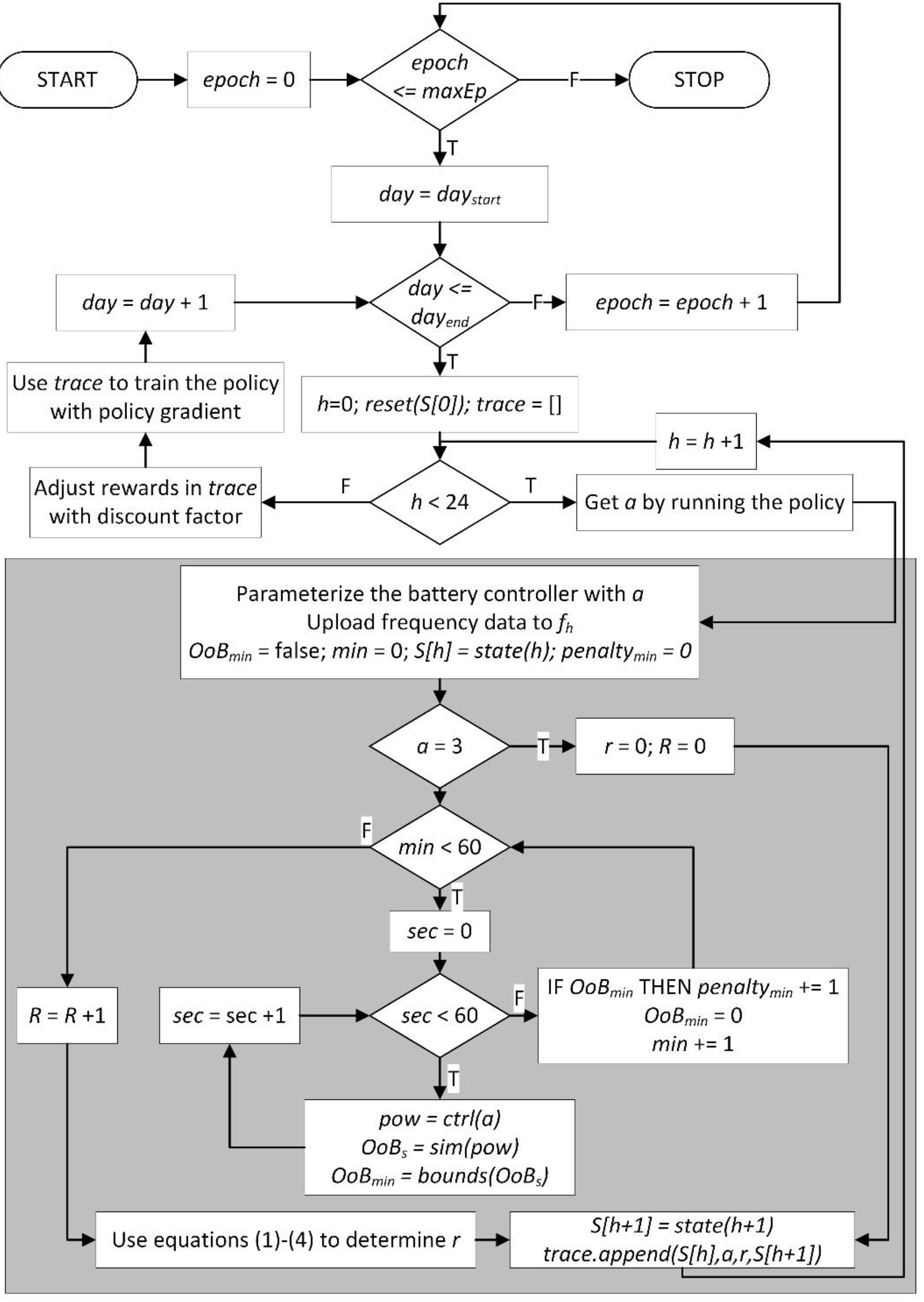
| reset(S[0]) | Resets the state variables at the beginning of the epoch |
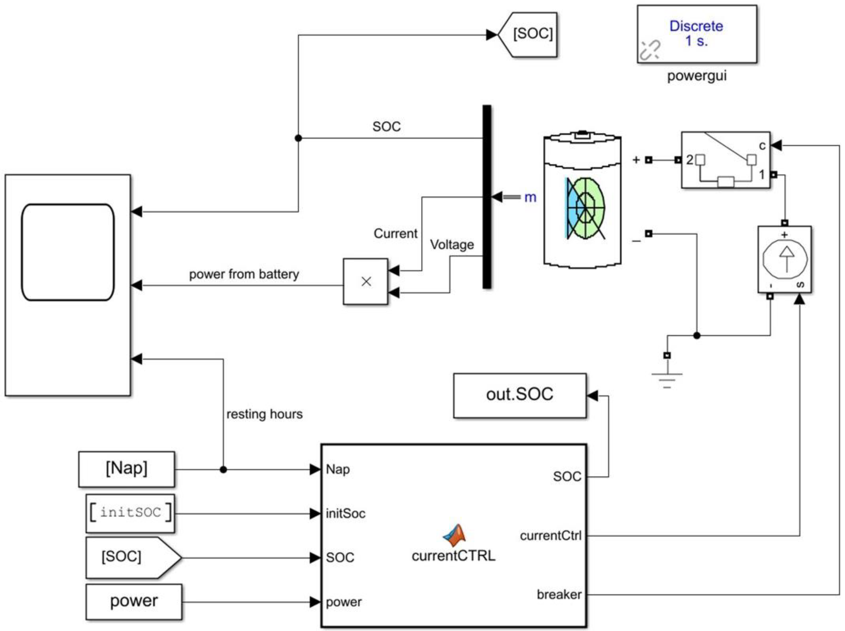
| pow = ctrl(a) | The parameter a is the frequency reserve capacity in kW that the bidding agent decided to bid on the frequency reserve market. The output pow is the discharge/charge power command to the battery from the battery controller. The output is determined according to the frequency data from fh and the FCR-N market technical specification [48]. |
| OoBs = sim(pow) | This function runs the battery simulation for one second, according to the pow charge/discharge command from ctrl(a). SoC is an internal state variable of the battery simulator. If the SoC goes OoB during this second, the OoBs output is true, otherwise false. |
| OoBmin = bounds(OoBs) | If OoBs is true, OoBmin is set true. Otherwise, no action. |
| capacity(a) | The capacity in MW of the bid corresponding to the action a taken by the agent. The capacity is 0 if a = 3, 0.6 MW if a = 2, 0.8 MW if a = 1 and 1.0 MW if a = 0. |
| S[h] = state(h) | Construct the state data structure S[h] with the current value of R and h. |
| Parameter | Value |
| Type | Lithium-ion |
| Nominal voltage | 1200 V |
| Rated capacity | 1400 Ah |
| Battery response time | 0.1 s |
| Simulate temperature effects | No |
| Simulate aging effects | No |
| Discharge parameters: determine from the nominal parameters of the battery | Yes |
| Hyperparameter | Value |
| Number of hidden layers | 1 |
| Number of nodes in input layer | 2 |
| Number of nodes in hidden layer | 20 |
| Number of nodes in output layer | 4 |
| Epsilon decay | 0.998 |
| Learning rate | 0.01 |
| Discount factor | 0.5 |
| Hidden layer activation function | Sigmoid |
| Output layer activation function | Softmax |
| Dropout | Not used |
| Optimizer | Adam |
Publisher’s Note: MDPI stays neutral with regard to jurisdictional claims in published maps and institutional affiliations. |
© 2021 by the authors. Licensee MDPI, Basel, Switzerland. This article is an open access article distributed under the terms and conditions of the Creative Commons Attribution (CC BY) license (https://creativecommons.org/licenses/by/4.0/).
Share and Cite
Aaltonen, H.; Sierla, S.; Subramanya, R.; Vyatkin, V. A Simulation Environment for Training a Reinforcement Learning Agent Trading a Battery Storage. Energies 2021, 14, 5587. https://doi.org/10.3390/en14175587
Aaltonen H, Sierla S, Subramanya R, Vyatkin V. A Simulation Environment for Training a Reinforcement Learning Agent Trading a Battery Storage. Energies. 2021; 14(17):5587. https://doi.org/10.3390/en14175587
Chicago/Turabian StyleAaltonen, Harri, Seppo Sierla, Rakshith Subramanya, and Valeriy Vyatkin. 2021. "A Simulation Environment for Training a Reinforcement Learning Agent Trading a Battery Storage" Energies 14, no. 17: 5587. https://doi.org/10.3390/en14175587
APA StyleAaltonen, H., Sierla, S., Subramanya, R., & Vyatkin, V. (2021). A Simulation Environment for Training a Reinforcement Learning Agent Trading a Battery Storage. Energies, 14(17), 5587. https://doi.org/10.3390/en14175587