Driving Factors and Future Prediction of Carbon Emissions in the ‘Belt and Road Initiative’ Countries

Abstract

‘Belt and Road Initiative’ (B&R) countries play critical roles in mitigating global carbon emission under the Paris agreement, but their driving factors and feasibility to reduce carbon emissions remain unclear. This paper aims to identify the main driving factors (MDFs) behind carbon emissions and predict the future emissions trajectories of the B&R countries under different social-economic pathways based on the extended STIRPAT (stochastic impacts by regression on population, affluence, and technology) model. The empirical results indicate that GDP per capita and energy consumption structure are the MDFs that promote carbon emission, while energy intensity improvement is the MDF that inhibits carbon emission. Population, as another MDF, has a dual impact across countries. The carbon emissions in all B&R countries are predicted to increase from SSP1 to SSP3, but emissions trajectories vary across countries. Under the SSP1 scenario, carbon emissions in over 60% of B&R countries can peak or decline, and the aggregated peak emissions will amount to 21.97 Gt in 2030. Under the SSP2 scenario, about half of the countries can peak or decline, while their peak emissions and peak time are both higher and later than SSP1, the highest emission of 25.35 Gt is observed in 2050. Conversely, over 65% of B&R countries are incapable of either peaking or declining under the SSP3 scenario, with the highest aggregated emission of 33.10 Gt in 2050. It is further suggested that decline of carbon emission occurs when the inhibiting effects of energy intensity exceed the positive impacts of other MDFs in most B&R countries.

1. Introduction

The ‘Belt and Road Initiative’ (B&R), initiated by China in 2013, aims to build a trade and infrastructure network connecting Asia with Europe and Africa along the ancient Silk Road. As of 2015, 65 countries signed this initiative to boost infrastructure, economy, trade, culture, and tourism. In 2015, the signatory countries accounted for 61.8% of the global population, consumed 50% of the world’s energy, and contributed 47% to the world’s gross domestic product (GDP) while emitting over 59% of the global CO₂ [1,2]. The average growth rate (5%) of carbon emissions in the above countries surpassed the average global rate (3%) by a significant margin during the last decade [3,4,5]. The surging economic development and cooperation across B&R countries translate into the increasing growth rate of CO₂ emissions. Under the Paris Agreement, with a global temperature control target of 2 °C/1.5 °C, the global carbon emissions need to be half that of their 2010 levels by the year 2050 [6,7]. With no exceptions, all 65 B&R countries are signatories to the Paris Agreement with established NDC (Nationally Determined Contribution) targets. The B&R countries need to take active measures to mitigate their future carbon emissions. Thus, it is necessary to predict the carbon emission trajectory of the B&R countries for assessing the feasibility of their emission reduction goals.

Existing studies on future carbon emissions have mostly been conducted on a regional or national level [8,9]. For instance, Wu et al. [10] assessed the carbon emission in BRICs countries and predicted that China would have the largest CO₂ emissions (9479 Mt) in 2020, while India and Brazil were predicted to emit 453 Mt and 300 Mt of CO₂, respectively. Wang et al. [11] predicted the CO₂ emissions of China and India in 2030, both of which will grow and reach to 10391Mt and 3395 Mt, respectively. Some studies have also predicted that China’s carbon emissions will peak in the range of 8000 Mt to 18,000 Mt from 2025 to 2040 [12,13,14]. However, to date, no work has predicted the carbon emissions of all B&R countries. It is worth noting that these predictions, to a large extent, are based on the cognition of socioeconomic factors (i.e., population, GDP, and energy intensity), which also regulate carbon emissions trajectories. Therefore, to obtain a scientifically robust prediction of emissions trajectory and peaking time, it is crucial to understand the driving factors of carbon emission in each country.

Several studies have shown that carbon emissions are highly related to socioeconomic factors, such as total population, urbanization, GDP per capita, industrial structure, and energy intensity [15,16,17,18]. However, how these factors impact the carbon emissions for B&R countries remains unknown. In addition, with the enhancement of economic globalization, economic and trade patterns have significantly changed across countries, but rarely has the literature studied factors such as foreign investment and trade openness that represent economic globalization. In addition, some widely used models, including the Logarithmic Mean Divisia Index (LMDI) model, Index Decomposition Analysis (IDA), as well as the Environment Impacts by Population, Affluence, and Technology (IPAT) model, either decompose carbon emission only into limited real-world factors or fail to track the non-linear relationships between carbon emissions and driving factors [13,19]. These limitations also lead to the under-examination of driving factors.

To fill the literature gap, this study aims to identify the main driving factors (MDFs) behind carbon emissions and predict the future emissions trajectories of the B&R countries under different social-economic pathways. To that end, we apply the extended STIRPAT model to identify the country-specific MDFs from eight potential drivers. Then, we use the identified MDFs to predict the future emission trajectory of B&R countries under three Shared Socioeconomic Pathways (SSPs). Finally, we explore the peak time and peak value of carbon emissions in the B&R countries under three SSP scenarios.

This paper is organized as follows: Section 2 provides critical reviews on the recent literature in this field. Section 3 describes the model and the data used in this study. Section 4 presents the results, and Section 5 displays the discussion. Finally, Section 6 addresses the conclusions and policy implications of our work.

2. Literature Review

Research studies that assess the driving factors of carbon emissions primarily examine the relationship between carbon emissions and socioeconomic factors [20,21,22,23]. The frequently analyzed representative factors include total population, urbanization level, GDP per capita, financial development, energy consumption structure, and energy intensity. For example, Shuai et al. [24] investigated the impact of total population, GDP per capita, and energy intensity on carbon emission in 125 countries and concluded that GDP per capita was the global key driving factor of carbon emission. Brizga [25] selected total population, GDP per capita, fossil energy consumption, and industry proportion as the potential driving factors to investigate the MDFs in former Soviet Union countries. Khan et al. [26] analyzed the influence of energy intensity, GDP per capita, financial development, and income inequality on carbon emission in three developing Asian countries. However, with the increase in globalization, additional less considered factors, such as foreign direct investment and trade openness, have also been recognized as exerting a rather prominent influence on carbon emission in some countries [27,28]. It is essential to investigate whether these factors have impacted the carbon emissions and the extent of their impacts.

However, some previously used models have limitations on adding additional factors. Some models are only capable of decomposing carbon emission into a fixed number of factors due to the limited model dimensions, while others may fail to detect the non-linear relationship between carbon emission and the additional driving factors. The STIRPAT model can not only quantify the impact of population, affluence, and technology on the environment, but can also add unlimited additional factors, such as the industrial structure, renewable energy consumption, service industry proportion, foreign direct investment, and trade openness. It provides the advantage of exploring potential driving factors of carbon emissions, making it a commonly used method to identify the driving factors of carbon emissions [29,30].

An increasing number of studies extended the STIRPAT model by adding and dropping variables to examine the relationship between driving factors and carbon emission [31] (

Table 1. Brief summary of previous literature for carbon emission used Extended STIRPAT models.

Authors	Study Areas	Period	MDFs and Result
			Population, Affluence, Technology Variables	Extend Variables
Li et al. (2011) [31]	China	1991–2009	Population (+), GDP per capita (+), Technology level (−)	Industrial structure (+), Urbanization (+)
Shafiei and Salim (2014) [32]	OECD countries	1980–2011	Population (+), GDP per capita (+), Energy intensity (+)	Renewable energy consumption (−), Non-renewable energy consumption (+), Urbanization (+ invert-U shaped)
Shuai (2018) [24]	China	1996–2015	Total Population (×), GDP per capita (+), Energy intensity (×)	Industry value added (+), Fixed assets investment (−), Urbanization (−), Renewable energy (−)
Salim et al. (2017) [33]	13 Asia countries	1980–2010	Population (+), GDP per capita (+), Non-renewable Energy Consumption (+)	Urbanization (−), Renewable energy (−), Trade liberalization (−)
Ghazali and Ali (2019) [27]	10 newly industrialized countries	1991–2013	Total Population (+), GDP per capita (+), Carbon intensity (+)	Energy mix (+), Trade openness (−)
Wang et al. (2017) [43]	China (Xinjiang)	1952–2012	Population (+), GDP per capita (+), Carbon intensity (−)	Industrialization (+), Tertiary industry proportion (−), Fixed assets investment (+), Trade openness (+), Energy consumption structure (+)
Wang et al. (2012) [44]	China(Beijing)	1997–2010	Population (#), GDP per capita (+), Energy intensity (−)	Urbanization (+), Industry proportion (+), Tertiary industry proportion (−), R&D output (−)
Wang et al. (2019) [45]	China (Guangdong)	1995–2014	Population (+), GDP per capita (+), Energy intensity (−)	Industrialization level (+), Fixed assets investment (−), Energy consumption structure (+)
Fan et al. (2006) [46]	99 countries	1975–2000	Population (+ in HI,-in UMI), GDP per capita (+), Energy intensity (+ in HI, LMI and LI, -in UMI)	Urbanization (− in HI)
Nguyen et al. (2019) [47]	33 emerging economies	1996–2014	Population (#), GDP per capita (+), Energy intensity (+)	Urbanization (−), Trade openness (+ in short run, - in long run), Foreign direct investiment (+)
Zhang and Zhou (2016) [48]	China	1995–2010	Population (+), GDP per capita (+), Energy intensity (−)	Urbanization (+), Industry structure (−), foreign direct investiment (−)
Inmaculada et al. (2011) [30]	93 developing countries	1975–2003	Population (+), GDP per capita (+), Energy Efficiency (−)	Urbanization (+I nverted-U shaped), Industrial Activity (+)
Roy (2017) [49]	India	1990–2016	Population (+), GDP per capita (+), Carbon intensity (−)	Energy demand (−), energy mix (+), fossil fuel energy intensity (+)
Poumanyvong and Kaneko (2010) [29]	99 countries	1975–2005	Population (+), GDP per capita (+), Energy intensity (−)	Urbanization (+), Share of industry in GDP (+ in HI), Share of services in GDP (×)
Sadorsky (2014) [50]	16emerging countries	1971–2009	Population (+), GDP per capita (+), Energy intensity (+)	Urbanization (×)

+ is positive effect, − is negative effect. (#) Variable not analysis in the study, (×): Variable is not significant and not the MDF, HI: High income level, UMI: upper-medium income level; LMI: lower-medium income.

). For example, Li et al. [32] extended the STIRPAT model by adding industry structure, urbanization, and technology level and found that technology level is the MDF inhibiting China’s carbon emissions while other factors are the MDFs promoting carbon emissions. Shafiei and Salim [33] used urbanization, renewable energy consumption, and non-renewable energy consumption to extend the STIRPAT model in OECD countries and concluded that all factors, except for renewable energy consumption, promote the increase of carbon emission. Furthermore, Salim et al. [34] applied urbanization, renewable energy, and trade liberalization to extend the STIRPAT model for 13 Asian countries and concluded that these factors are the MDFs that exert a positive influence on carbon emission reduction. Similarly, Ghazali and Ali [27] employed trade openness and energy mix to extend the STIRPAT model for 10 newly industrialized countries and suggested that the energy mix promotes carbon emissions, while trade openness inhibits carbon emissions.

Combining the STIRPAT model with the socioeconomic scenario can be used to predict future carbon emissions under the Shared Socioeconomic Pathways (SSPs) [35,36]. These are established to facilitate the integrated analysis of future climate impacts, vulnerabilities, adaptation, and mitigation pathways and describe different climate futures that cover additional possible and internally consistent socioeconomic developments [37,38,39,40]. The SSPs describe five plausible future pathways in mitigation and adaptation challenges by narrating alternative social, economic, and technical aspects in the 21st century and provide a new pathway for future carbon emissions prediction. Specifically, the first three SSPs correspond to low, medium, and high challenges to both mitigation and adaptation, which can also cover the previously commonly used Low, BAU (business as usual), and High scenarios. Several studies used this as a new scenario framework to predict future carbon emission trajectory and provided crucial information for the 2 °C/1.5 °C temperature control target [41,42].

3. Materials and Methods

This study applied the extended STIRPAT model to identify the MDFs governing carbon emissions and then predicted the future emissions trajectory of B&R countries. Firstly, using the historical carbon emissions data from World Bank (1990–2014) [1], the correlation among carbon emissions and eight potential driving factors (total population, urbanization, GDP per capita, energy consumption structure, industry structure, energy intensity, renewable energy consumption, and trade openness) was tested. Then, the factors that passed the Pearson correlation test were used to run the extended STIRPAT model to identify the MDFs in each B&R country. Lastly, by combining the identified MDFs and scenario assumptions, a country-specific STIRPAT model was established to predict future carbon emissions.

3.1. STIRPAT Model

This paper employed the improved non-linear stochastic regression STIRPAT model, which is created based on the IPAT model and describes the impact of population, affluence, and technology on environmental pressure [51]. It overcomes the unit elasticity assumption. In other words, the STIRPAT model assumes that there is a non-linear relationship between the variables, which can statistically analyze the non-proportionate impacts of variables on the environment. The mathematical formulation of the STIRPAT model is shown in the following Equation (1):

$$I=\alpha P^a{A}^b{T}^{c}e$$

(1)

After taking the natural logarithm, it is written in the linear form as Equation (2):

$$\ln I=\ln \alpha +a\ln P+b\ln A+c\ln T+\ln e$$

(2)

where I represents the environmental pressure (carbon emission); P, A and T denote the factor of population, affluence, and technology, respectively (independent variable); α is the intercept; a, b, c represent the elastic coefficients of P, A, and T; e is the random error term. Equation (2) could be further extended by integrating additional driving factors as:

$$\begin{array}{l}\ln I_{\mathrm{i}}=\ln a_1+a_2\ln T{P}_i+a_3\ln U{R}_i+a_4\ln R{G}_i+a_5\ln E{S}_i\\ \begin{array}{cc}& \end{array}+a_6\ln I{S}_i+a_7\ln E{I}_i+a_8\ln R{E}_i+a_9\ln T{O}_i+\ln e\end{array}$$

(3)

where the subscript i stands for the country samples, a₁ is the constant, a₂, a₃…a₉ are the elastic coefficients, TP is the total population in thousands, UR is urbanization (%), RG is the GDP (gross domestic product) per capita (constant 2011 USD), ES is the energy consumption structure(%), IS is the industry structure (%), EI is the energy intensity (kg of oil equivalent per constant 2011 PPP$), RE is the renewable energy consumption (%), and TO is the trade openness (%). A detailed description of the variables has been shown in

Table 2. The detailed driving factors in the STIRPAT model.

Variable	Short Name	Description	Unit
C	Carbon emissions	Carbon emissions from energy-relate	Kt
TP	Population	total population	thousand people
UR	Urbanization	The ratio of urban population in total population	%
RG	GDP per capita	Real GDP per capita	constant 2011 USD
ES	Energy consumption structure	The ratio of fossil energy in total energy consumption	%
IS	Industry structure	The industrial value-added over the total GDP	constant 2011 US (% of GDP)
EI	Energy intensity	Energy consumption per GDP	kg of oil equivalent per constant 2011 PPP$
RE	Renewable energy consumption	The ratio of renewable energy in total energy consumption	%
TO	Trade openness	The ratio of trade (exports and imports) in GDP	% of GDP

. It should be noted that the correlation of each potential driving factor (mentioned in Table 2) with the carbon emissions has been tested through Pearson’s correlation analysis.

The elastic coefficients need to be solved by regression methods. However, the OLS (Ordinary Least Squares) regression may lead to multiple collinearities problem, since the variance inflation factors (VIFs) of many countries were over 10, and for some, even above 100. Therefore, to eliminate the multi-collinearity, the PLS (Partial Least Squares) regression was employed for each country. The significant factors were defined as the MDFs, for which a specified STIRPAT model of each country was established and used to predict its future carbon emissions.

3.2. Predicting Scenarios

Three SSPs scenarios, namely, SSP1, SSP2, and SSP3, representing low, medium, and high challenges to both mitigation and adaptation, are integrated into the STIRPAT model to predict future carbon emissions. SSP1 is a sustainable road that leads to low challenges to both mitigation and adaptation. This scenario constitutes an inclusive development with a relatively higher increase in income, urbanization, trade, and cooperation, but lower growth in population and consumption. SSP1 is oriented towards low fossil fuel consumption and lower energy intensity, which can basically achieve the 1.5 °C temperature control target. SSP2 presents medium challenges to both mitigation and adaptation. It is a scenario in which the above-mentioned socioeconomic development factors follow the middle of the business-as-usual road trends. On the contrary, SSP3 describes a regional rivalry road due to more focus on competitiveness and security among regions, and it leads to high challenges to both mitigation and adaptation [39]. The assumptions on the variable among three SSP scenarios are shown in

Table 3. The three SSP scenarios assumptions.

Scenario	Mitigation Challenges	Adaptation Challenges	Population Growth	GDP per Capita	Urbanization	Industry Structure	Energy Consumption Structure	Energy Intensity	Trade Openness	Renewable Energy
SSP1	Low	Low	Low	High	High	High	Low	Low	High	High
SSP2	Medium	Medium	Medium	Medium	Medium	Medium	Medium	Medium	Medium	Medium
SSP3	High	High	High	Low	Low	Low	High	High	Low	Low

.

3.3. Data

In this study, the historical data of annual CO₂ emissions and socioeconomic factors of B&R countries from 1990 to 2014 were used. The annual CO₂ emissions (Kt), the proxy of the dependent variables, were obtained from the World Bank database [1]. The eight related independent variables, including total population (thousand people), GDP per capita (measured as GDP divided by midyear population, constant 2011 USD), energy intensity (measured as energy use per GDP, kg of oil equivalent per constant 2011 PPP$), urbanization (the ratio of the urban population in the total population, %), energy consumption structure (the share of fossil energy consumption in total energy consumption, %), renewable energy consumption (the share of renewable energy consumption in total energy consumption, %), industry structure (the share of industry value added to GDP, %), and trade openness (the ratio of trade, including import and export to GDP, %) from 1990 to 2014 are stated in Table 2. The data of all eight independent variables were derived from the Word Bank database [1]. Factors related to GDP were converted into the 2011 fixed price for eliminating the effect of price rise. It should be noted that the B&R countries in this paper refer to those countries that signed the ‘Belt and Road Initiative’ with China before 2016. Considering the availability of data, only 60 B&R countries, except East Timor, Afghanistan, the Maldives, Syria, and Palestine, were analyzed in this study (see Appendix A 

Table A1. List of 60 B&R countries and classification.

High income level countries(16 countries with per captia > US$ 122,76 in 2010	Slovenia, Singapore, Saudi Arabia, Qatar, Kuwait, Israel, Brunei, Bahrain, United Arab Emirates, Czech Republic, Hungary, Oman, Poland, Slovakia, Estonia, Croatia,
Upper middle income level groups(21 countries with per captia GNP between US$ 3976 and US$ 122,75 in 2010	Lithuania, Latvia, Russia, Turkey, Malaysia, Kazakhstan, Lebanon, Romania, Bulgaria, Montenegro, Iran, Belarus, Azerbaijan, Serbia, Thailand, China, Bosnia and Herzegovina, Macedonia, Iraq, Turkmenistan, Albania
low middle income level groups(23 countries with per captia < US$ 3975 in 2010	Jordan, Armenia, Indonesia, Ukraine, Georgia, Sri Lanka, Mongolia, Egypt, Bhutan, Philippines, Moldova, Uzbekistan, India, Vietnam, Yemen, Laos, Pakistan, Myanmar, Kyrgyzstan, Cambodia, Bangladesh, Tajikistan, Nepal

). Furthermore, these countries were divided into three groups, including the lower-middle-income group (LMI), the upper-middle-income group (UMI), and the high-income group (HI), according to the World Bank list of economies of June 2010 [52].

In addition, the data of socioeconomic assumptions (i.e., GDP per capita, urbanization, and total population) used to predict from 2015 to 2050 were obtained from the SSP database (https://tntcat.iiasa.ac.at/SspDb/dsd?Action=htmlpage&page=80, accessed on 1 February 2021), taken from the International Institute for Applied Systems Analysis (IIASA) and the Wittgenstein Center for Demography and Global Human Capital model [53,54,55,56]. The data of energy consumption structure (fossil energy consumption, renewable energy consumption) and technology level (energy intensity) were obtained from the SSP database, which was taken from the Integrated assessment models (IAM) scenarios model [39]. Other variables like industrial structure and trade openness were designed according to the description of the SSPs [36,39].

4. Results

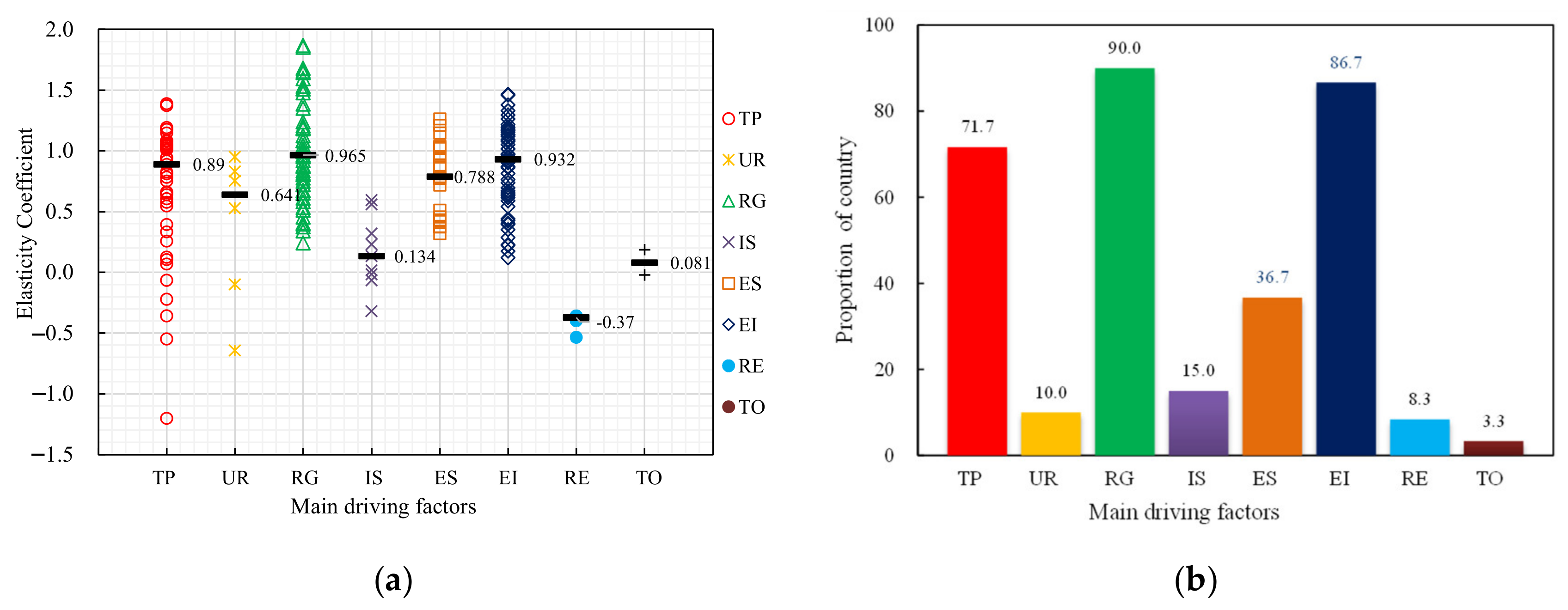
4.1. Main Driving Factors

The selected MDFs of the B&R countries identified through regression analysis are listed in Appendix A 

Table A2. The coefficient of empirical STIRPAT model after PLS regression.

Countries	cons	lnTP	lnUR	lnRG	LnIS	lnEC	lnEI	lnRE	lnTO	R2	Residual
Qatar	10.158 ***	0.607 ***	0.018 *	0.045 **	0.091	0.102 **	0.442 ***	−0.013	0.075 *	0.989	0.0132
Singapore	8.879 ***	0.125 ***	0.001	0.078 *	−0.203 *	0.041	0.828 ***	0.124	−0.121	0.82	0.07197
Kuwait	−17.01 ***	−0.065 ***	0.174 *	1.143 ***	0.085	0.025	1.218 ***	−0.148 *	0.035	0.994	0.0225
Brunei	14.164 ***	0.257 ***	0.003	0.674 ***	0.323	0.022	1.409 ***	−0.184	−0.017	0.933	0.1122
United Arab Emirates	4.592 ***	0.826 ***	−0.015 *	0.006 **	−0.091	1.021 ***	0.025 *	−0.044	0.007 *	0.937	0.17732
Israel	−11.11 ***	0.64 ***	0.211 **	1.176 ***	0.018 ***	0.026	1.263 ***	−0.031	−0.013 *	0.992	0.01939
Slovakia	12.863 ***	−0.547 ***	0.193	−0.094	0.231 ***	0.426 ***	0.244	−0.011	−0.006	0.973	0.01538
Bahrain	−2.216 ***	0.89 ***	0.141	0.654 ***	-	0.103	1.297 ***	−0.065	−0.037	0.889	0.11917
Czech	1.083 ***	−0.357 ***	0.256 *	0.724 ***	−0.043	0.498 **	1.168 ***	−0.105 *	0.088	0.973	0.01783
Oman	−18.252 ***	1.177 ***	−0.413	1.546 ***	0.112	−0.046	0.765 ***	——	0.132	0.966	0.1148
Saudi Arabia	−17.435 ***	0.394 ***	−0.074 **	1.176 ***	0.226 **	−0.034 **	0.672 ***	0.084	0.109 *	0.967	0.09436
Slovenia	10.829 ***	−1.501 ***	0.085	0.721 ***	0.034	0.378 ***	1.18 ***	0.054	0.362	0.887	0.0263
Estonia	−6.467 ***	0.018 **	−0.812 *	1.048 ***	0.029	0.114	1.195 ***	−0.232 *	−0.333	0.983	0.00362
Hungary	2.563 ***	0.084	0.179	0.013 ***	−0.015 ***	0.951 ***	1.332 ***	0.026 *	0.101	0.987	0.01687
Croatia	−6.036 ***	0.018 *	0.01	1.086 ***	0.175	0.207	1.466 ***	−0.357 ***	0.022	0.868	0.08974
Poland	−14.934 ***	1.153 ***	−0.121 **	0.962 ***	−0.021	0.772 ***	1.18 ***	−0.013 *	0.014	0.995	0.00451
Lithuania	−12.62 ***	0.947 ***	0.084	0.818 ***	0.34	1.044 **	1.073 ***	−0.618 **	0.927	0.967	0.01873
Latvia	−34.45 ***	0.752 ***	1.258 **	1.207 ***	−0.169	0.155 *	1.379 ***	−0.534 ***	−0.017	0.99	0.01178
Russia	−16.176 ***	1.052 ***	−0.098 ***	1.083 ***	0.032	0.474 *	1.155 ***	−0.019	−0.004 *	0.995	0.00658
Azerbaijan	−5.849 ***	0.657 ***	−0.498	0.967 ***	−0.046 *	0.131	0.863 ***	0.041	0.513 *	0.98	0.07517
Turkey	−8.645 ***	0.118 *	0.951 ***	1.016 ***	−0.006	0.432 ***	0.94 ***	−0.023	0.103	0.999	0.00864
Malaysia	−4.812 ***	−0.221 ***	−0.076 **	0.875 ***	−0.055	0.319 ***	0.353 ***	0.022	0.108	0.993	0.05212
Kazakhstan	−6.586 ***	1.178 ***	0.035	0.405 ***	0.561 ***	0.488 *	0.146 *	−0.398 ***	−0.051	0.979	0.04586
Lebanon	−12.394 ***	0.917 ***	−0.014	0.611 ***	0.11	0.512 ***	0.645 ***	−0.078	−0.096	0.951	0.06774
Romania	−12.389 ***	0.813 ***	−0.166 **	0.535 ***	−0.016	0.923 ***	1.018 ***	−0.063 *	0.101	0.998	0.01045
Bulgaria	−7.909 ***	0.071	−0.067 *	0.837 ***	0.036	1.490 ***	0.95 ***	−0.176 *	−0.062	0.959	0.032
Montenegro	−10.988 ***	0.105	0.071	1.595 ***	0.025	——	0.905 ***	——	−0.05	0.984	0.02048
Iran	−13.611 ***	1.149 ***	0.02 *	0.398 ***	0.034	0.107	0.427 ***	−0.017 *	−0.07	0.99	0.04029
Belarus	−2.443 ***	0.093 **	0.031 *	0.183 ***	0.32 ***	0.415 *	0.97 ***	−0.183 *	−0.024 ***	0.938	0.0313
Serbia	−3.471 ***	0.121 *	0.092	0.079	−0.321 ***	0.952 ***	0.397 ***	−0.041	0.003	0.996	0.0068
Thailand	−3.919 ***	0.03 **	−0.642 ***	1.681 ***	0.003	1.032 ***	0.057 **	−0.068 **	−0.02 **	0.997	0.0213
China	−2.277 ***	.066 *	−0.202 *	1.190 ***	0.596 **	−0.108	1.121 ***	−0.379 ***	0.121 *	0.998	0.02014
Bosnia and Herzegovina	−5.905 ***	0.029	−0.085 *	0.994 ***	−0.015	1.21 ***	0.972 ***	−0.037	0.021	0.997	0.0213
Macedonia, FTR	−21.588 ***	1.026 ***	0.097 *	0.697 ***	0.05	0.184 *	0.654 ***	0.126	0.136	0.964	0.05432
Iraq	−6.248 ***	0.664 ***	0.032	0.34 ***	0.089	0.104	0.883 **	−0.062	0.026 *	0.895	0.06551
Turkmenistan	−12.143 ***	0.081 **	0.828 ***	1.182 ***	−0.064 ***	0.021 *	0.815 ***	−0.024 *	0.084	0.998	0.01199
Albania	−11.477 ***	0.194 **	−0.111	1.646 ***	0.123	0.197	1.452 ***	−0.081 **	0.012	0.945	0.09761
Jordan	−7.321 ***	0.809 ***	0.034 *	0.778 ***	0.103	0.091	0.923 ***	−0.132	0.053	0.99	0.02983
Armenia	−3.602 ***	−0.297 *	−0.143 *	0.751 ***	—	0.787 ***	0.842 ***	−0.167	−0.125	0.97	0.05471
Indonesia	−13.251 ***	1.085 ***	0.213 **	0.805 ***	0.049	0.011	0.175 ***	0.149	−0.014	0.949	0.09458
Ukraine	−25.384 ***	1.041 ***	0.469 *	0.673 ***	−0.094	1.107 ***	0.789 ***	−0.002	0.047	0.988	0.02896
Georgia	0.633 ***	−0.275	0.236	0.922 ***	0.396	−0.464	0.615 ***	−0.36 ***	−0.011	0.955	0.0233
Sri Lanka	−61.542 ***	1.04 ***	0.147	0.43	−0.046	0.458 ***	0.723 ***	−0.206 **	0.012	0.99	0.04897
Mongolia	−16.658 ***	1.75 ***	−0.495 *	1.351 ***	0.108 *	0.196 *	1.121 ***	−0.372 *	−0.150 *	0.897	0.05987
Egypt	−9.978 ***	1.08 ***	−0.616 **	0.952 ***	−0.318 *	−0.083	1.094 ***	−0.821 **	0.003	0.976	0.0596
Bhutan	−60.459 ***	0.334 ***	0.23	1.511 ***	0.2	—	0.886 ***	−0.039 *	0.172	0.98	0.07517
Philippines	−16.415 ***	1.011 ***	−0.033 *	1.386 ***	−0.098	0.719 ***	1.136 ***	−0.451 **	−0.032	0.99	0.02666
Moldova	−31.11 ***	0.310 *	0.169 *	1.013 ***	−0.231 *	0.884 ***	−0.08 ***	−0.103	−0.31	0.951	0.03236
Uzbekistan	−13.889 ***	0.943 ***	0.199 *	1.241 ***	0.134 ***	0.062	1.133 ***	0.172	0.284	0.934	0.02114
India	−10.272 ***	0.546 ***	0.298 *	1.126 ***	−0.005 *	1.044 ***	1.089 ***	−0.038	0.016	0.998	0.01731
Vietnam	−4.247 ***	0.152 **	0.243 **	0.808 ***	0.054	1.264 ***	0.914 ***	−0.159	−0.025	0.997	0.01433
Yemen	−13.511 ***	1.086 ***	−0.087 *	1.479 ***	0.01	−0.05 **	0.976 ***	−0.033 **	−0.036	0.979	0.04076
Laos	−25.634 ***	1.064 ***	0.755 ***	0.883 ***	0.036	——	——	0.518 *	0.115	0.98	0.01191
Pakistan	−17.179 ***	1.041 ***	0.518 *	0.657 ***	−0.001	−0.645 ***	0.634 ***	−0.018	0.098	0.995	0.02122
Myanmar	−16.204 ***	1.391 ***	0.073	1.534 ***	−0.072	0.127	0.404 ***	−0.126	0.192	0.938	0.05651
Kyrgyzstan	−18.158 ***	0.578 ***	−0.011	0.454 ***	−0.053	0.375 ***	0.696 ***	−0.04 *	0.023	0.988	0.03076
Cambodia	−10.642 ***	−0.003 **	0.021 **	1.508 ***	−0.036	1.015	0.739 ***	−0.135	−0.063	0.995	0.03316
Bangladesh	−18.885 ***	1.375 ***	1.132 ***	0.872 ***	−0.057	0.735 *	0.389 ***	−0.28 **	0.098	0.998	0.02146
Tajikistan	−42.779 ***	0.783 ***	0.11	1.854 ***	0.106	−0.4	0.872 ***	0.103 **	−0.045	0.938	0.02081
Nepal	−8.037 ***	−0.153 *	−0.179 *	1.868 ***	0.106	0.783 ***	0.043 *	−0.005 *	0.185 ***	0.986	0.01761
Median		0.89	0.792	0.965	0.134	0.788	0.932	−0.379	0.081

Selected ***, **, and * denote the correlation is significant at the 0.01, 0.05, and 0.1 level, respectively.

, and their elasticity coefficients are plotted in Figure 1. We show that the elasticity coefficients of GDP per capita, energy consumption structure, and energy intensity are positive in all B&R countries, which indicate positive effects on carbon emission. The negative elasticity coefficient of renewable energy shows its inhibitive impact on carbon emissions. Other factors such as population, urbanization, industry structure, and trade openness may have opposing effects on different countries due to their positive or negative elasticity coefficients. Figure 1b counts the number of countries having a specific factor as its MDF. It can be seen that the GDP per capita was the most featured factor (90% of countries), followed by energy intensity and population. The carbon emissions of over 71.7% of countries are dominated by these three factors. On the other hand, urbanization, industry structure, and trade openness were selected as the MDFs least number of times, with smaller elasticity coefficients, which implies their limited influence on the carbon emissions in B&R countries.

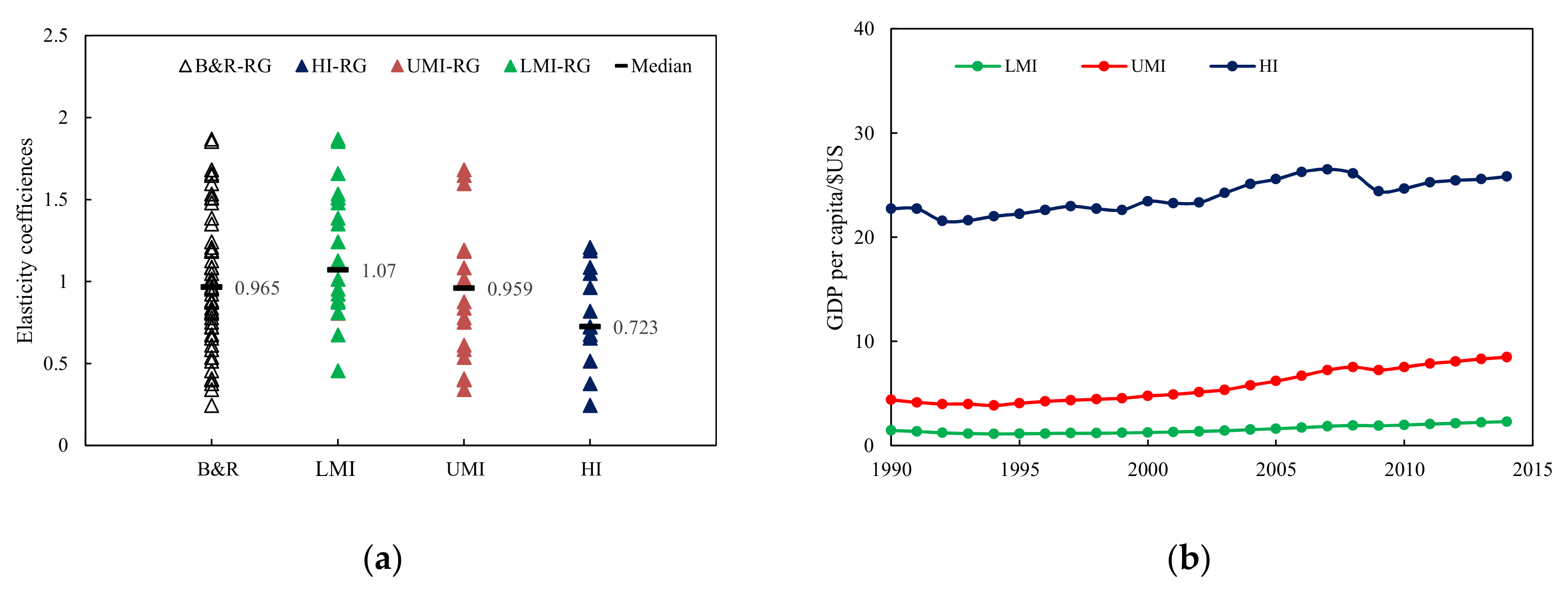
4.1.1. The Influence of GDP per Capita

GDP per capita is the main factor responsible for increasing carbon emission in B&R countries. The elasticity coefficients, as shown in Figure 2a, are all positive, with a median value of 0.965, which means every 1% increase in GDP per capita will lead to a 0.965% increase in carbon emissions. As seen from Figure 2b, from 1990 to 2014, the GDP per capita of all three income groups increased gradually by 58%, 93%, and 19% for HI, UMI, and LMI countries, respectively. However, the gap in GDP per capita between different income groups remained significant. Therefore, if GDP keeps growing at a similar pace, the impact of GDP per capita on carbon emissions is expected to further intensify in these countries. It is interesting to note that the elasticity coefficient is slightly higher for LMI countries (1.07) and UMI countries (0.959) than HI countries (0.723). This indicates that the impact of GDP per capita may slightly weaken with the increase of income level. The GDP per capita does not feature in the MDFs of Qatar, the United Arab Emirates, and Singapore, indicating that the carbon emissions of these countries have decoupled from their economies. This result is consistent with the Environmental Kuznets Curve (EKC) hypothesis, which states that when the economy of a country reaches a certain level, its effect on carbon emissions will gradually decline and possibly even decouple in the future [57,58].

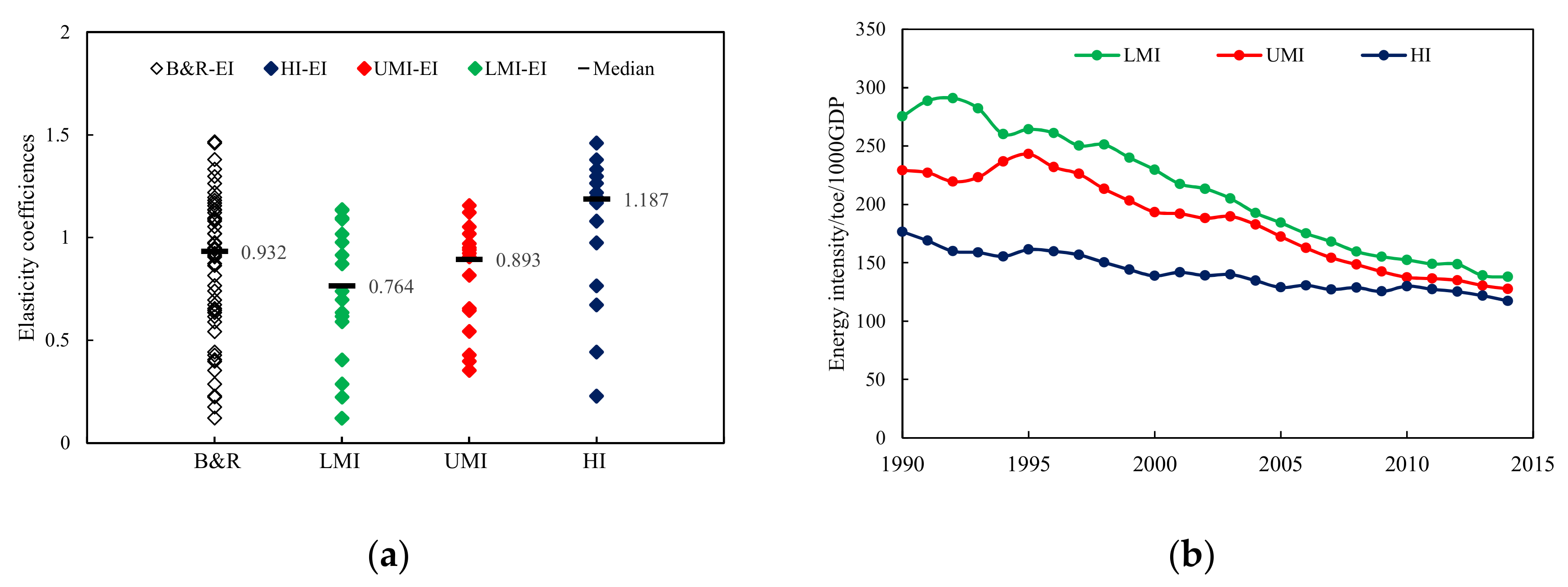
4.1.2. The Influence of Energy Intensity

Energy intensity is the second most crucial MDF within B&R countries. The influence of energy intensity on the carbon emissions of countries belonging to different income groups is consistent. As shown in Figure 3a, the elasticity coefficients of all countries are positive, with a median value of 0.93. The median value of the elasticity coefficient is slightly higher for HI countries (1.187) and UMI countries (0.959) than LMI countries (0.764). This suggests that the impact of energy intensity becomes more critical when the income increases. The gradual decrease in the energy intensity from 1990 to 2014 (Figure 3b) led to the mitigation of carbon emissions. Every 1% improvement (decrease) in energy intensity has reduced 0.93% of carbon emissions. Meanwhile, the energy intensities of all three income groups appear to have reached a bottleneck under current technology and have merged around 130 toe/1000 USD since 2010. If the trend continues, the impact of energy intensity on carbon emissions may be less significant in the future.

4.1.3. The Influence of Population

As one of the MDFs after GDP per capita and energy intensity, the influence of the population for different income groups shows high variability. As shown in Figure 4a, the elasticity coefficients fluctuated from negative to positive in different countries, which implies the dual impacts of the population on carbon emissions. The median coefficients of LMI (1.041) and UMI (0.813) groups are much higher than those of the HI group (0.394). At the same time, the growth rate of the population of LMI (45% from Figure 3b) is much larger than the corresponding rates of UMI and HI groups. This suggests that the impact of the population on carbon emission will decrease as the income increases. The elasticity coefficients are negative for some of the countries belonging to the HI group, such as Slovenia and Kuwait. Therefore, for these countries, population growth may even inhibit carbon emissions. Our results are in agreement with Shuai et al. [24] in that the impact of the population on carbon emissions might be opposite in different income groups.

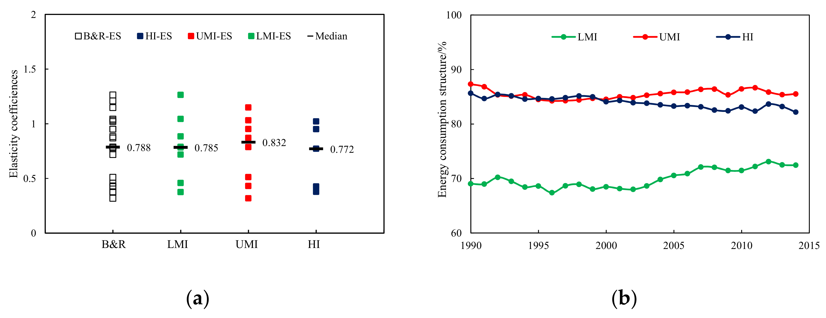
4.1.4. The Influence of Energy Consumption Structure

Energy consumption structure represents the ratio of fossil fuel consumption over the total energy consumption. Energy consumption structure is also one of the MDFs within B&R countries with a consistent influence on different income groups. The elasticity coefficients were found to be similar for different income groups with a median value of 0.788, as shown in Figure 5a. It means that every 1% increment in the proportion of fossil fuel consumption would result in an 0.788% increase in carbon emissions in B&R countries. However, as shown in Figure 5b, energy consumption structure in all three income groups did not change significantly from 1990 to 2014. The fossil energy consumption in HI groups showed a slightly declining trend, while others have increased slightly. Especially for countries in LMI groups, whose fossil fuel consumption increased by 4.9% since 2000, the impact of energy consumption structure on carbon emissions is highly likely to be intensified in the future.

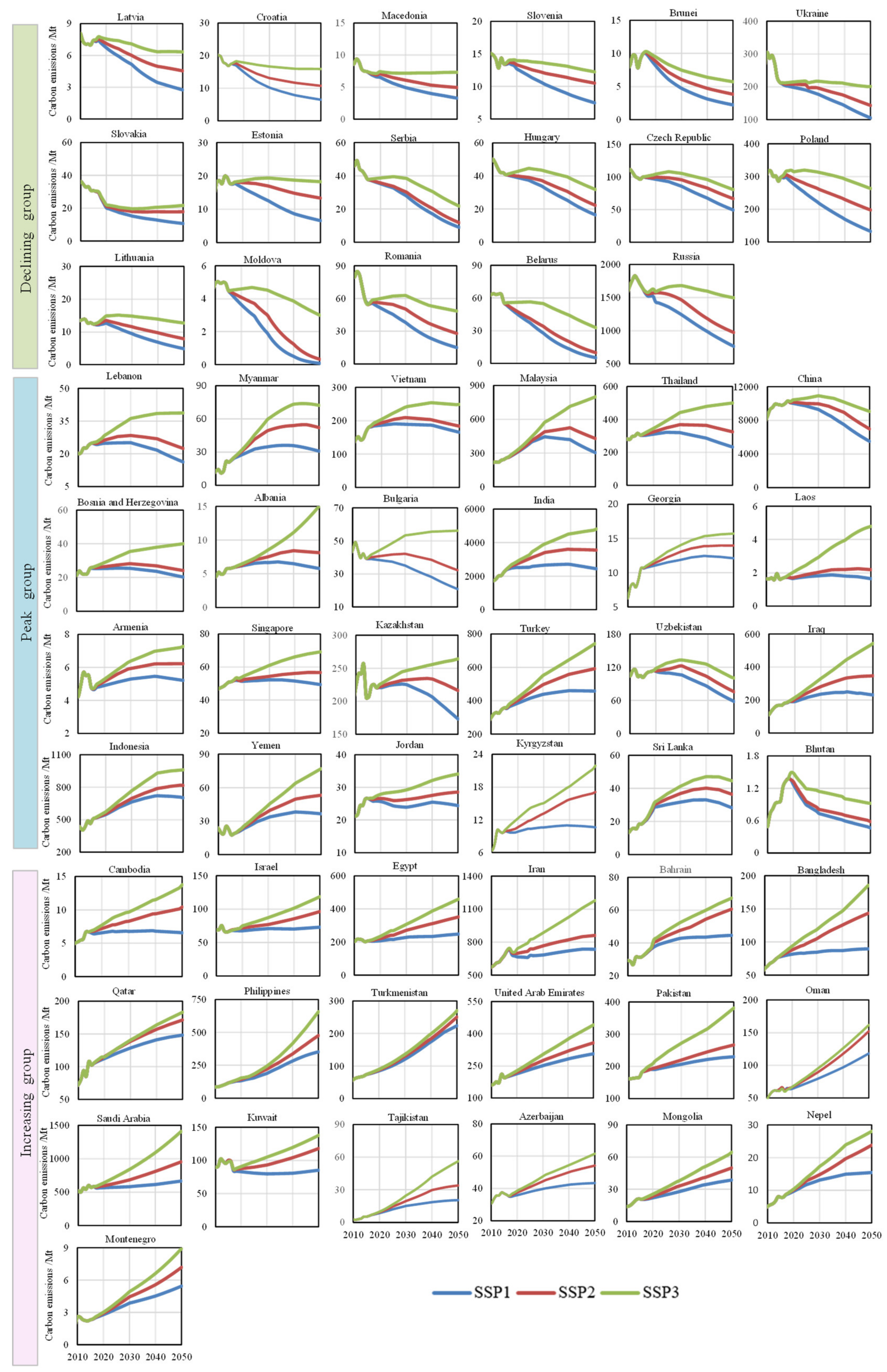
4.2. Predicting Carbon Emission at the National Level

Based on the specified empirical STIRPAT model by country, we predicted their carbon emission under three different SSP scenarios. The aggregated carbon emissions of B&R countries in key years have been shown in

Table 4. Carbon emissions of B&R countries in different scenarios.

Scenarios	Aggregated Carbon Emissions/Gt
	2020	2030	2040	2050
SSP1	21.43	21.97	21.22	19.72
SSP2	22.41	24.52	25.27	25.35
SSP3	23.43	27.88	30.64	33.10

. In general, carbon emissions under the SSP3 scenario are the highest, followed by SSP2, and the SSP1 is the lowest. Under the SSP1 scenario, the aggregated carbon emissions in B&R countries are expected to peak in 2030, with total emissions of 21.97 Gt. Under the SSP2 scenario, the aggregated emission will continue to increase until 2040, and then enter a plateau period with 25 Gt carbon emissions per year. Under the SSP3 scenario, carbon emissions will increase dramatically and are unlikely to peak until 2050. The highest aggregated carbon emissions will reach 33.10 Gt in 2050.

According to the emission trajectories of three SSP scenarios, as shown in Figure 6, 60 B&R countries can be classified into the following three groups:

(1)

Declining group: This group is characterized by a gradual decline in carbon emissions from 2015–2050;

(2)

Peaking group: The carbon emissions of this group can peak before 2050;

(3)

Increasing group: The carbon emission will continue to grow from 2015–2050.

It should be noted that the groups are not consistent in all scenarios.

Under the SSP1 scenario, 17 countries, most of which are HI and LMI, show a decreasing trend in carbon emissions at a rate between 1.36% and 6.56%. The fastest reduction happens in Belarus, whose carbon emissions are predicted to reduce from 55.6 Mt in 2014 to 5.2 Mt in 2050. In contrast, the slowest reduction occurs in Romania, whose emission reduces from 55.78 Mt to 34.51 Mt. Under the SSP2 scenario, 17 countries maintain a consistent downward trend. However, the decreasing rate of carbon emissions is expected to slow down to an average of 1.94%. The decreasing rate of carbon emissions in Romania is expected to reduce to 0.25%. Under the SSP3 scenario, carbon emissions of only eight countries show a decreasing trend. At the same time, the annual average rate further decreased to 0.39%. Some UMI countries such as Belarus, Serbia, Russia, Romania, Lithuania, and Moldova turned into the peaking group.

On the other hand, around 20 countries, most of which are UMI and LMI countries, under SSP1 and SSP2, show an increasing trend in carbon emissions. Under SSP1, the average annual growth rate is approximately 1.4%, with Turkmenistan (3.2%) and Kuwait (0.07%) showing the fastest and slowest growth rates, respectively. Under SSP2, Kazakhstan, Turkey, Uzbekistan, Iraq, Yemen, Jordan, and Kyrgyzstan were added to the emissions increasing groups. The average annual growth rate rose slightly to 1.8%. The fastest growth rate (4.3%) was observed for Tajikistan, while the slowest growth rate (0.2%) was observed for Jordan. However, under SSP3, more than 30 countries show an increasing trend in carbon emissions, and the average annual growth rate increased to 2.3%. The slowest rate (0.7%) was found for the United Arab Emirates, while the fastest growth rate (5.8%) was observed in Tajikistan. It is noted that the two largest carbon emission countries, China and India, also switched to the increasing group under SSP3. Although their growth rates of 1.0% and 2.0%, respectively, were lower than the average, the cumulative increased carbon emissions due to scenario change may reach 39700 Mt and 24182 Mt, respectively.

As shown in Figure 7, both the timing and amount of peak emissions vary significantly among different SSPs. Under SSP1 scenarios, over 38% (23/60) of B&R countries will reach peak emissions (Figure 7a). Furthermore, UMI countries reach their peaks earlier than LMI countries. Most UMI countries (i.e., China, Thailand) tend to reach peak around 2030, with peak emissions of 12,661.9 Mt. In contrast, most LMI countries (i.e., India, Kazakhstan, Turkey, Indonesia) are expected to peak around 2040, with a total peak emission of 4743.6 M. Under the SSP2 scenario, countries such as Uzbekistan, Iraq, Yemen, Jordan, Kazakhstan, Turkey, and Kyrgyzstan will no longer reach peak emissions. Therefore, the carbon emissions of only one-fourth of B&R countries (16/60) can still reach a peak (Figure 7b), most of them being UMI and LMI countries. However, their peak emissions are both more massive and occur later when compared to those under SSP1. The peak times of countries such as Malaysia, China, India, Singapore, and Albania have been delayed by nearly 10 years in comparison to SSP1, resulting in 1871 Mt more emissions. The carbon emissions of the remaining 11 countries such as Lebanon, Myanmar, Vietnam, Thailand and Indonesia peak 5 years late, with an additional peak emission of 177 Mt when compared to SSP1. Under the SSP3 scenario, the carbon emissions of only 21% (13/60) of B&R countries are likely to peak by 2050 (Figure 7c). It should be noted that only four countries (Lebanon, Myanmar, Vietnam, and Sri Lanka) remained from the peaking group under SSP2. In comparison, the other nine countries transformed from the declining group under SSP2 and belong to the peaking group in SSP3. Furthermore, the peak timing of those four remaining countries is 2–4 years later compared with SSP2, leading to additional 99 Mt emissions.

5. Discussion

The effects of MDFs on carbon emission under different SSP scenarios were further quantified by multiplying the elasticity coefficient and their changes (% increase) during 2015–2050, as shown in Figure 8. Overall, the predicted emission trajectories are highly dependent on the combined effects of different MDFs, which is consistent with Le quere et al. [59]. The effects of energy intensity improvement are the dominant factor for emissions entering into the reduction path. For the countries in the declining group, the inhibiting effect of energy intensity improvement on carbon emissions is around 40–60%, which is 1.16 times the total positive effects of other factors such as GDP per capita and the energy consumption structure. Referring to the previous results (Figure 2), the countries in the declining groups are mostly from the HI levels, for whom the impact of GDP per capita on carbon emissions has been weakened or even decoupled.

On the other hand, as the effects of GDP per capita become larger, the carbon emissions of these countries are more likely to increase to a peak value and then decrease. The peak will occur when the inhibiting effects of energy intensity improvement offset the positive effects of other MDFs. This can also be explained by the EKC hypothesis. Carbon emissions decrease with the increase in income when it reaches a certain level (a turning point). While, for countries whose GDP per capita continues growing and has not reached a turning point from 2015–2050, their emissions will continue increasing.

The effects of the population are the other contributor to a continuous increase in carbon emissions and the inability to reach peak. For the countries in the increasing group, the positive effects of the population become more significant than the other two groups, and their average effects even reach up to 67%. Most of these countries belong to the LMI group, whose population is expected to increase consistently (referring to Figure 4), thereby increasing carbon emissions. On the contrary, for countries such as Latvia, Slovenia, and the Czech Republic in the HI group, the impact of the population turns negative, which is consistent with Section 4.1.3. This again proves the double-edged effect of the population on carbon emissions. Furthermore, the effects of energy consumption on carbon emissions are negligible for most of the B&R countries. However, for some LMI countries, such as Armenia, Kyrgyzstan, and India, their effect of energy consumption is an important driving force for entering into the increasing group.

In addition, the assumptions about the growth or decrease rate of MDFs have also been recognized as another reason for the changes in carbon emission trajectories. As shown in Figure 8, the effects of energy intensity significantly decrease from SSP1 and SSP2 to SSP3, which contribute to the increased carbon emissions from SSP1 to SSP3. This might have been caused by the differences in the assumptions of the energy intensity decrease rate, which was 2% in SSP1, 1.5% in SSP2, and 1.0% in SSP3. However, as shown in Section 4.1.3, energy intensity improvement may be subtle in the future, which implies the possible overprediction of carbon emission. In addition, the effects of the population have increased by 12.8% from SSP2 to SSP3. This may have been caused by the assumed average annual population growth rate of 0.5% and 0.8% in SSP2 and SSP3, respectively. Especially for countries such as Iraq, Yemen, Kazakhstan, and Jordan, the average population growth rate even reached 1.5% (in SSP2) and 1.8% (in SSP3), transitioning them to the increasing group from the peaking group.

6. Conclusions

In this paper, we applied extended STIRPAT models by assembling historical CO₂ emissions to explore the MDFs behind carbon emissions in 60 B&R countries. We also predict the emission trajectories under three SSP scenarios over the next 45 years (2015–2050). The following conclusions are drawn from this study.

GDP per capita, population, energy consumption structure, and energy intensity are the four MDFs occurring in most of the B&R countries. On the other hand, the effects of urbanization, industrial structure, renewable energy, and trade openness on carbon emissions are less important. The GDP per capita and energy consumption structure are the main MDFs that promote carbon emissions and have a significant impact on LMI countries. The energy intensity improvement is the MDF that inhibits carbon emissions and has a significant impact on HI countries. The population was found to have a dual effect on carbon emissions, with its effect gradually weakening and even becoming negative from LMI to HI countries.

The aggregated carbon emissions of the 60 B&R countries are the largest under the SSP3 scenario (33.1 Gt), followed by 25.38 Gt under SSP2, and 21.97 Gt under the SSP1 scenario. The emission trajectories under three scenarios exhibit the following trends: declining, peaking, and increasing. Under the SSP1 scenario, the carbon emissions of over 60% of B&R countries can either peak or decline. The emissions of UMI countries were found to peak earlier than LMI countries. Under the SSP2 scenario, carbon emissions of over half of the countries can peak or decline. However, their peak emissions are higher by 2048 Mt and delayed by 5 to 10 years in comparison to SSP1. Conversely, under the SSP3 scenario, the carbon emissions of over 65% of countries are incapable of either peaking or declining but reveal an increasing trend.

In addition, we found that the effect of MDFs and its inherent assumptions are two main reasons that caused the changes in carbon emission trajectories in the future. For B&R countries, the decline in carbon emissions is due to the inhibiting effects of energy intensity exceeding the positive impacts of other MDFs. Carbon emissions can reach their peak when the inhibitory effects of energy intensity offset the positive effects of other MDFs. In the absence of this effect, carbon emissions will continue to increase. In addition, the assumptions on the growth or decrease rate of MDFs are another reason for variations in the future carbon emission trajectories. Especially for countries belonging to the LMI groups, the increase in the population growth rate is the main reason that facilitates their entry into the emissions increasing group.

Therefore, this paper may provide decision makers with the following policy advice to effectively mitigate carbon emissions in the future: B&R countries should focus on their MDFs and design strategies that are in line with each country.

For countries that take energy intensity as the dominant factor and are incapable of peaking in at least one scenario, it is critical to improve their energy intensity by either regulating the industrial structure or promoting advanced low-carbon technologies. For countries that take GDP per capita as the dominant factor and are unlikely to peak in at least one scenario, it is important to change the economic development mode and decouple carbon emissions from the economy as early as possible. For countries that take population as the dominant factor and whose carbon emissions continue increasing regardless of the scenarios, it is essential to control the growth rate of population properly and improve public awareness of environmental protection. For countries that take energy consumption structure as the dominant factor and are incapable of peaking in at least one scenario, it is imperative to adjust the energy consumption structure for reducing fossil energy usage.

References

1. World Bank Data Indicator (WDI). Available online: http://data.worldbank.org.cn (accessed on 1 January 2021).
2. Zhang, Y.-J.; Jin, Y.-L.; Shen, B. Measuring the Energy Saving and CO2 Emissions Reduction Potential under China’s Belt and Road Initiative. Comput. Econ. 2018, 55, 1095–1116. [Google Scholar] [CrossRef]
3. Belt and Road Portal. 2017. Available online: https://www.yidaiyilu.gov.cn/ (accessed on 2 February 2021).
4. Belt and Road Portal. 2018. Available online: https://www.yidaiyilu.gov.cn/ (accessed on 2 February 2021).
5. Fan, J.-L.; Da, Y.-B.; Wan, S.-L.; Zhang, M.; Cao, Z.; Wang, Y. Determinants of carbon emissions in ‘Belt and Road initiative’ countries: A production technology perspective. Appl. Energy 2019, 239, 268–279. [Google Scholar] [CrossRef]
6. Climate Change 2014: Synthesis Report. Available online: https://www.ipcc.ch/site/assets/uploads/2018/05/SYR_AR5_FINAL_full_wcover.pdf (accessed on 2 February 2021).
7. Climate Change 2018: Special Report on Global Warming of 1.5 °C. Available online: https://unfccc.int/topics/science/workstreams/cooperation-with-the-ipcc/ipcc-special-report-on-global-warming-of-15-degc (accessed on 2 February 2021).
8. Ahmadi, M.H.; Ramezanizadeh, M.; Nazari, M.A.; Kheradmand, S.; Shamshirband, S. Carbon Dioxide Emission Prediction of Four CIS Countries by Applying a Correlation and GMDH Artificial Neural Network. Preprints 2019, 2019060227. [Google Scholar] [CrossRef]
9. Hosseini, S.M.; Saifoddin, A.; Shirmohammadi, R.; Aslani, A. Forecasting of CO2 emissions in Iran based on time series and regression analysis. Energy Rep. 2019, 5, 619–631. [Google Scholar] [CrossRef]
10. Wu, L.; Liu, S.; Liu, D.; Fang, Z.; Xu, H. Modelling and forecasting CO2 emissions in the BRICS (Brazil, Russia, India, China, and South Africa) countries using a novel multi-variable grey model. Energy 2015, 79, 489–495. [Google Scholar] [CrossRef]
11. Wang, Q.; Li, S.; Pisarenko, Z. Modeling carbon emission trajectory of China, US and India. J. Clean. Prod. 2020, 258, 120723. [Google Scholar] [CrossRef]
12. Zhao, X.; Du, D. Forecasting carbon dioxide emissions. J. Environ. Manag. 2015, 160, 39–44. [Google Scholar] [CrossRef] [PubMed]
13. Fang, K.; Tang, Y.; Zhang, Q.; Song, J.; Xu, A. Will China peak its energy-related carbon emissions by 2030? Lessons from 30 Chinese provinces. Appl. Energy 2019, 255, 113852. [Google Scholar] [CrossRef]
14. Zhou, N.; Price, L.; Yande, D.; Creyts, J.; Khanna, N.; Fridley, D.; Lu, H.; Feng, W.; Liu, X.; Hasanbeigi, A.; et al. A roadmap for China to peak carbon dioxide emissions and achieve a 20% share of non-fossil fuels in primary energy by 2030. Appl. Energy 2019, 239, 793–819. [Google Scholar] [CrossRef]
15. Li, J.S.; Zhou, H.W.; Meng, J.; Yang, Q.; Chen, B.; Zhang, Y.Y. Carbon emissions and their drivers for a typical urban economy from multiple perspectives: A case analysis for Beijing city. Appl. Energy 2018, 226, 1076–1086. [Google Scholar] [CrossRef]
16. Chapman, A.; Fujii, H.; Managi, S. Key Drivers for Cooperation toward Sustainable Development and the Management of CO2 Emissions: Comparative Analysis of Six Northeast Asian Countries. Sustainability 2018, 10, 244. [Google Scholar] [CrossRef] [Green Version]
17. de Alegría, I.M.; Basañez, A.; de Basurto, P.D.; Fernández-Sainz, A. Spain’s fulfillment of its Kyoto commitments and its funda-mental greenhouse gas (ghg) emission reduction drivers. Renew. Sustain. Energy Rev. 2016, 59, 858–867. [Google Scholar] [CrossRef]
18. Li, M.Y.; Weng, Y.Y.; Duan, M.S. Emissions, energy and economic impacts of linking China’s national ETS with the EU ETS. Appl. Energy 2019, 235, 1235–1244. [Google Scholar] [CrossRef]
19. Wang, C.H.; Chen, N.; Chan, S.L. A gravity model integrating high-speed rail and seismic-hazard mitigation through landuse planning: Application to California development. Habitat Int. 2017, 62, 51–61. [Google Scholar] [CrossRef]
20. Xiao, B.; Niu, D.; Guo, X. The Driving Forces of Changes in CO2 Emissions in China: A Structural Decomposition Analysis. Energies 2016, 9, 259. [Google Scholar] [CrossRef] [Green Version]
21. Yao, C.; Feng, K.; Hubacek, K. Driving forces of CO2 emissions in the G20 countries: An index decomposition analysis from 1971 to 2010. Ecol. Inform. 2015, 26, 93–100. [Google Scholar] [CrossRef]
22. Chong, C.H.; Tan, W.X.; Ting, Z.J.; Liu, P.; Ma, L.; Li, Z.; Ni, W. The driving factors of energy-related CO2 emission growth in Malaysia: The LMDI decomposition method based on energy allocation analysis. Renew. Sustain. Energy Rev. 2019, 115, 109356. [Google Scholar] [CrossRef]
23. Jiang, X.; Guan, D. Determinants of global CO2 emissions growth. Appl. Energy 2016, 184, 1132–1141. [Google Scholar] [CrossRef] [Green Version]
24. Shuai, C.; Chen, X.; Wu, Y.; Tan, Y.; Zhang, Y.; Shen, L. Identifying the key impact factors of carbon emission in China: Results from a largely expanded pool of potential impact factors. J. Clean. Prod. 2018, 175, 612–623. [Google Scholar] [CrossRef]
25. Brizga, J.; Feng, K.; Hubacek, K. Drivers of CO2 emissions in the former Soviet Union: A country level IPAT analysis from 1990 to 2010. Energy 2013, 59, 743–753. [Google Scholar] [CrossRef]
26. Khan, A.Q.; Saleem, N.; Fatima, S.T. Financial development, income inequality, and CO2 emissions in Asian countries using STIRPAT model. Environ. Sci. Pollut. Res. 2018, 25, 6308–6319. [Google Scholar] [CrossRef] [PubMed]
27. Ghazali, A.; Ali, G. Investigation of key contributors of CO2 emissions in extended STIRPAT model for newly industrialized countries: A dynamic common correlated estimator (DCCE) approach. Energy Rep. 2019, 5, 242–252. [Google Scholar] [CrossRef]
28. Zhang, Y.; Zhang, S. The impacts of GDP, trade structure, exchange rate and FDI inflows on china’s carbon emissions. Energy Policy 2018, 120, 347–353. [Google Scholar] [CrossRef]
29. Poumanyvong, P.; Kaneko, S. Does urbanization lead to less energy use and lower CO2 emissions? A cross-country analysis. Ecol. Econ. 2010, 70, 434–444. [Google Scholar] [CrossRef]
30. Inmaculada, M.Z.; Antonello, M. The impact of urbanization on CO2 emissions: Evidence from developing countries. Ecol. Econ. 2011, 70, 1344–1353. [Google Scholar]
31. Liu, D.; Xiao, B. Can China achieve its carbon emission peaking? A scenario analysis based on STIRPAT and system dynamics model. Ecol. Indic. 2018, 93, 647–657. [Google Scholar] [CrossRef]
32. Li, H.; Mu, H.; Zhang, M.; Li, N. Analysis on influence factors of China’s CO2 emissions based on Path–STIRPAT model. Energy Policy 2011, 39, 6906–6911. [Google Scholar] [CrossRef]
33. Shafiei, S.; Salim, R.A. Non-renewable and renewable energy consumption and CO2 emissions in OECD countries: A compar-ative analysis. Energy Policy 2014, 66, 547–556. [Google Scholar] [CrossRef] [Green Version]
34. Salim, R.; Rafiq, S.; Shafiei, S. Urbanization, Energy Consumption, and Pollutant Emission in Asian Developing Economies: An Empirical Analysis. Available online: http://hdl.handle.net/10419/163205 (accessed on 1 May 2021).
35. Böhmelt, T. Employing the shared socioeconomic pathways to predict CO2 emissions. Environ. Sci. Policy 2017, 75, 56–64. [Google Scholar] [CrossRef]
36. Riahi, K.; van Vuurenb, D.P.; Krieglerc, E.; Edmondsd, J.; O’Neille, B.C.; Fujimori, S.; Bauer, N.; Calvin, K.; Dellink, R.; Fricko, O.; et al. The shared socioeconomic pathways and their energy, land use, and greenhouse gas emissions implications: An overview. Glob. Environ. Chang. 2016, 42, 153–168. [Google Scholar] [CrossRef] [Green Version]
37. Ebi, K.L.; Hallegatte, S.; Kram, T.; Arnell, N.W.; Carter, T.R.; Edmonds, J.; Kriegler, E.; Mathur, R.; O’Neill, B.C.; Riahi, K.; et al. A new scenario framework for climate change research: Background, process, and future directions. Clim. Chang. 2013, 122, 363–372. [Google Scholar] [CrossRef] [Green Version]
38. Kriegler, E.; O’Neill, B.C.; Hallegatte, S.; Kram, T.; Lempert, R.J.; Moss, R.; Wilbanks, T. The need for and use of socioeconomic scenarios for climate change analysis: A new approach based on shared socio-economic pathways. Glob. Environ. Chang. 2012, 22, 807–822. [Google Scholar] [CrossRef]
39. O’Neill, B.C.; Kriegler, E.; Kristie, L.E.; Kemp-Benedict, E.; Riahi, K.; Rothman, D.S.; van Ruijven, B.J.; van Vuuren, D.P.; Birkmann, J.; Kok, K.; et al. The roads ahead: Narratives for shared socioeconomic pathways describing world futures in the 21st century. Glob. Environ. Chang. 2017, 42, 169–180. [Google Scholar] [CrossRef] [Green Version]
40. Ruijven, B.J.; Levy, M.A.; Agrawal, A.; Biermann, F.; Birkmann, J.; Carter, T.R.; Ebi, K.L.; Garschagen, M.; Jones, B.; Jones, R.; et al. Enhancing the relevance of shared socioeconomic path-ways for climate change impacts, adaptation and vulnerability research. Clim. Chang. 2014, 122, 481–494. [Google Scholar] [CrossRef] [Green Version]
41. Marangoni, G.; Tavoni, M.; Bosetti, V.; Borgonovo, E.; Capros, P.; Fricko, O.; Gernaat, D.E.H.J.; Guivarch, C.; Havlik, P.; Huppmann, D.; et al. Sensitivity of projected long-term CO2 emissions across the Shared Socioeconomic Pathways. Nat. Clim. Chang. 2017, 7, 113–117. [Google Scholar] [CrossRef]
42. Wei, Y.M.; Han, R.; Liang, Q.M.; Yu, B.Y.; Yao, Y.F.; Xue, M.M.; Zhang, K.; Liu, L.-J.; Peng, J.; Yang, P.; et al. An integrated assessment of INDCs under Shared Socioeco-nomic Pathways: An implementation of C3IAM. Nat. Hazards 2018, 92, 585–618. [Google Scholar] [CrossRef] [Green Version]
43. Wang, S.; Wang, J.; Li, S.; Fang, C.; Feng, K. Socioeconomic driving forces and scenario simulation of CO2 emissions for a fast-developing region in China. J. Clean. Prod. 2019, 216, 217–229. [Google Scholar] [CrossRef]
44. Wang, C.; Wang, F.; Zhang, X.; Yang, Y.; Su, Y.; Ye, Y.; Zhang, H. Examining the driving factors of energy related carbon emissions using the extended STIRPAT model based on IPAT identity in Xinjiang. Renew. Sustain. Energy Rev. 2017, 67, 51–61. [Google Scholar] [CrossRef]
45. Wang, Z.; Yin, F.; Zhang, Y.; Zhang, X. An empirical research on the influencing factors of regional CO2 emissions: Evidence from Beijing city, China. Appl. Energy 2012, 100, 277–284. [Google Scholar] [CrossRef]
46. Fan, Y.; Liu, L.-C.; Wu, G.; Wei, Y.-M. Analyzing impact factors of CO2 emissions using the STIRPAT model. Environ. Impact Assess. Rev. 2006, 26, 377–395. [Google Scholar] [CrossRef]
47. Nguyen, C.P.; Schinckus, C.; Su, T.D. Economic integration and CO2 emissions: Evidence from emerging economies. Clim. Dev. 2019, 12, 369–384. [Google Scholar] [CrossRef]
48. Zhang, C.G.; Zhou, X. Does foreign direct investment lead to lower CO2 emissions? Evidence from a regional analysis in China. Renew Sustain. Energy Rev. 2016, 58, 943–951. [Google Scholar] [CrossRef]
49. Roy, M.; Basu, S.; Pal, P. Examining the driving forces in moving toward a low carbon society: An extended STIRPAT analysis for a fast growing vast economy. Clean Technol. Environ. Policy 2017, 19, 2265–2276. [Google Scholar] [CrossRef]
50. Sadorsky, P. The effect of urbanization on CO2 emissions in emerging economies. Energy Econ. 2014, 41, 147–153. [Google Scholar] [CrossRef]
51. Dietz, T.; Rosa, E.A. Rethinking the environmental impacts of population, affluence, and technology. Hum. Ecol. Rev. 1994, 1, 277–300. [Google Scholar]
52. World Bank. Data. 2011. Available online: http://data.worldbank.org/indicator%3E (accessed on 2 February 2021).
53. Fricko, O.; Havlik, P.; Rogelj, J.; Klimont, Z.; Gusti, M.; Johnson, N.; Kolp, P.; Strubegger, M.; Valin, H.; Amann, M.; et al. The marker quantification of the Shared Socioeconomic Pathway 2: A middle-of-the-road scenario for the 21st century. Glob. Environ. Chang. 2017, 42, 251–267. [Google Scholar] [CrossRef] [Green Version]
54. Samir, K.C.; Wolfgang, L. The human core of the shared socioeconomic pathways: Population scenarios by age, sex and level of education for all countries to 2100. Glob. Environ. Chang. 2017, 42, 181–192. [Google Scholar]
55. Jesús, C.C. Income projections for climate change research: A framework based on human capital dynamics. Glob. Environ. Chang. 2017, 42, 226–236. [Google Scholar]
56. Jiang, L.; O’Neill, B.C. Global urbanization projections for the Shared Socioeconomic Pathways. Glob. Environ. Chang. 2017, 42, 193–199. [Google Scholar] [CrossRef] [Green Version]
57. Grossman, G.; Krueger, A. Environmental Impacts of a North American Free Trade Agreement. Natl. Bur. Econ. Res. 1991, 3914. [Google Scholar] [CrossRef]
58. Shafik, N.; Bandyopadhyay, S. Economic Growth and Environmental Quality: Timeseries and Cross-Country Evidence; World Bank Publications: Washington, DC, USA, 1992. [Google Scholar]
59. Le Quéré, C.; Korsbakken, J.I.; Wilson, C.; Tosun, J.; Andrew, R.; Andres, R.J.; Canadell, J.G.; Jordan, A.; Peters, G.P.; Van Vuuren, D.P. Drivers of declining CO2 emissions in 18 developed economies. Nat. Clim. Chang. 2019, 9, 213–217. [Google Scholar] [CrossRef] [Green Version]
Figure 1. The elasticity coefficients of MDFs and its proportion: (a) The elasticity coefficients of MDFs; (b) The proportion of countries having the factor as one of their MDFs.
Energies 14 05455 g001
Figure 2. The elasticity coefficiences of GDP per capita and its changes in different income groups: (a) The elasticity coefficiences of GDP per capita in three income groups; (b) The changes in GDP per capita in three income groups from 1990–2014.
Energies 14 05455 g002
Figure 3. The elasticity coefficiences of energy intensity and its changes in different income groups: (a) The elasticity coefficiences of energy intensity in three income groups; (b) The changes in the energy intensity of three income groups from 1990–2014.
Energies 14 05455 g003
Figure 4. The elasticity coefficiences of population and its changes in different income groups: (a) The elasticity coefficiences of the population in B&R countries; (b) The changes in the population of three income groups from 1990–2014.
Energies 14 05455 g004
Figure 5. The elasticity coefficients of energy consumption and its changes in different income groups: (a) The elasticity coefficiences of energy consumption structure in B&R countries; (b) The changes in the energy consumption structure of three income groups from 1990–2014.
Energies 14 05455 g005
Figure 6. Carbon emissions of 60 B&R countries under different SSPs. Plots are categorized by emission trajectories belonging under SSP1. The green, blue, and pink label on left of picture represent declining group, peak group, and in-creasing group, respectively.
Energies 14 05455 g006
Figure 7. Peak emission and time for 60 B&R countries under (a) SSP1, (b) SSP2, (c) SSP3.
Energies 14 05455 g007aEnergies 14 05455 g007b
Figure 8. The effects of MDFs in 60 B&R countries. The countries belonging to the decreasing group are marked with a green background, the peaking group is marked with a blue background, and the increasing group is marked with a pink background.
Energies 14 05455 g008