Evolution of Fundamental Price Determination within Electricity Market Simulations ^†

Abstract

Electricity prices are the key instrument for coordinating electricity markets. For long-term market analyses, price determination based on fundamental unit commitment simulations is required. Within the European wholesale market, electricity prices result from a market clearing, which finds a welfare-optimal price–quantity tuple considering a coupling of multiple market areas with limited transmission capacity. With increasing exchange capacities in Europe, the precise modeling of the market coupling is required. Many market simulation models use multi-stage approaches with a separation of market coupling and price determination. In this paper, we analyze a new single-stage approach that combines both steps and theoretically and empirically demonstrate its precision by a backtest. For this purpose, we compare a simulated versus a historical electricity price distribution. Moreover, we explain the necessary adjustments for future regulatory developments of the European electricity market regarding flow-based market coupling and propose a concept for the application of future regulatory developments. We demonstrate further developments using a future scenario.

1. Introduction

The prediction of electricity spot prices is essential for electricity market participants as prices have a crucial impact on operational and investment decisions. For short-term predictions, regression models are often used. For a long-term horizon, fundamental market models are better suited due to expected structural changes, such as coal phase-outs, and the expansion of renewable capacities in the course of the targeted decarbonization as declared in the Paris Agreement [1] (cf. [2,3]).

Fundamental price determinations are generally based on unit commitment (UC) models. These models can be part of scenario expansion planning models as in [4] or used in market operation models. These operation models are often applied to future scenarios to evaluate concrete expansion measures concerning generation units or grid elements. Such models also enable the analysis of the integration of new market participants, e.g., virtual power plants or assessing political decisions regarding regulatory measures. In all investigations, prices are ultimately at the center of attention. For example, price convergence between market areas is an indicator for welfare gains due to changes in expansion capacity. Furthermore, the evaluation of returns’ structure from assets is directly dependent on market prices.

Market simulations model international electricity markets and usually assume competitive markets. This implies a welfare-optimized market outcome [5]. Thus, fundamental market simulations are based on optimization problems. In this paper, the focus is on electricity markets within the European interconnected system. The European electricity market is connected via implicit market coupling according to the concept of the ‘Price Coupling of Regions’ [6]. For an accurate representation of this market, the bidding behavior of all individual market participants must be depicted in detail. This contains restrictions on the operation of generation and storage units which are often non-linear, e.g., binary on–off decisions. This results in individual optimization models for each unit. Moreover, the cross-market electricity exchange which is based on implicit market coupling has a significant impact on the overall system as exchange volumes increase, especially due to grid expansion. Market coupling contains systemic constraints connecting the individual subproblems. This leads to the high complexity of the full optimization problem, which can be reduced by the application of mathematical decomposition approaches. Additionally, multi-stage approaches are often used [7,8,9,10]. In the first stage, all market areas within market coupling are considered with simplified constraints. Usually, all non-linear constraints are neglected. A further reduction in complexity can result from the aggregation of generation units outside the focus market areas [11,12]. In the second stage, the focus market areas are considered in detail with full constraints using fixed exchange schedules of the first stage. Consequently, market coupling can be neglected at this stage.

In the case of a linear optimization problem, electricity prices can be derived from the dual solution of the optimization problem. If non-linear constraints are applied in the second stage, this is not possible. One possibility would be to derive the prices from the first stage neglecting detailed power plants’ constraints. Instead, many approaches use a Lagrangian decomposition in the second stage [7,8,9]. Most of these models focus on dispatch optimization and do not aim to determine electricity prices, or prices are derived at a subsequent stage. In [8], the Lagrangian multipliers are treated as electricity prices.

In a multi-stage approach, each market price is determined separately. However, there is actually a dependence between prices and exchange flows: gaps between the prices of different market areas decrease with an increasing exchange. In terms of welfare maximization, exchange capacity must be fully used if market prices differ, as shown in [13]. The market algorithm provides a price alignment if exchange capacity is available. This dependency cannot be modeled in a multi-stage approach if exchange schedules are fixed. For example, further power plants constraints applied in the second stage can limit the export potential of a market area. Moreover, we show in this paper that even if the actual exchange schedules are applied, prices might not be correct. The problem is that the bids of power plants cannot be considered in the merit order of other markets and this leads to price distortions. The solution of the optimization problem via multi-stage approaches has the disadvantage of the detailed power plant characteristics not being able to influence the commitment decision across market areas. Most solutions for this problem are based on post adjustment as in [14]. However, this solution cannot guarantee the correct dependency of prices and exchange schedules. According to these previous approaches, there was a lack of market simulation models which combine a detailed cross-market power plant optimization with an endogenous electricity price determination.

A full consideration of prices and exchange schedules can only be ensured if prices and exchange schedules are determined within the same stage. Since the closed formulations of the problem are not applicable, a single-stage decomposition approach is necessary. Such an approach is given by [15]. The proposed concept is also based on a Lagrangian decomposition. However, in contrast to multi-stage approaches, multiple Lagrangian multipliers are used in parallel. This allows an overall market optimization analogous to the spot exchange using the EUPHEMIA algorithm [16].

Market coupling in the European electricity market is subject to many regulatory changes in recent years. An important step was the replacement of the net transfer capacity (NTC) approach with flow-based market coupling (FBMC) in central western Europe in April 2015. FBMC was developed for the more efficient utilization of existing exchange capacity in order to increase market welfare. Therefore, FBMC has an impact on electricity exchange schedules and on power plants’ dispatch. This has been empirically shown by parallel run results [17] and in several studies [18,19,20,21]. The resulting changes in electricity generation have also had an impact on the prices. Until this step, however, there was no effect on the price determination itself.

In November 2020, there was a significant change in the relationship between electricity exchange and prices. Previously, only exchange from the cheaper to the more expensive market area was possible. This is also referred to as ‘flow-based intuitive’. In this case, a cross-market price determination is only possible with regard to bilateral exchange. This approach was replaced by ‘flow-based plain’, which also allows counterintuitive flows. These flows occur in order to generate more exchange capacity by compensating other exchange flows [22].

This new approach makes price determination more complex as prices are not a result of bilateral exchange anymore. This means that the overall system must be considered in order to identify price adjustments that are necessary to achieve welfare gains which in turn affect the decomposition approaches. We propose a method to determine correct prices in this case. To the best of the authors’ knowledge, no previous approach has combined a detailed power plant dispatch with market coupling, both NTC and FBMC, endogenously. The aim of this paper was to explain and evaluate a concept that meets both criteria. This detailed determination of prices offers added value for the analysis of future scenarios of the energy system.

The rest of the paper is organized as follows. In Section 2, we explain the new single-stage approach and compare it with previous multi-stage approaches. Section 3 deals with the further adjustments for FBMC. Exemplary results are shown in Section 4. The relevance of single-stage market clearing models has been already shown via a backtest for 2014 under a NTC regime in [23]. A high precision of this model with respect to historical prices can be proofed. In this paper, we extend the application of the proposed single-stage approach by simulating future scenarios using FBMC. We show the impact of FBMC and counterintuitive flows and demonstrate which adjustments are necessary within the market simulation approach for a precise price determination. The results are discussed in Section 5. Section 6 gives a conclusion and an outlook.

2. From Multi-Stage to Single-Stage Market Models

This section focuses on the methods of market simulation approaches assuming full deterministic market optimization.

In general, inputs for this type of model are:

• All generation and storage units of the market with their respective operational limitations and costs;
• The electric load resulting from available transmission capacities on the interconnecting power lines;
• Constraints of the market coupling resulting from available transmission capacities on the interconnecting power lines;

The maximization of market welfare is analogous to the minimization of operational costs for load-covering if the demand is inelastic. The optimal solution implies the market outcome, which is composed of:

• Schedules of generation and storage units;
• The electricity exchange;
• Resulting market prices.

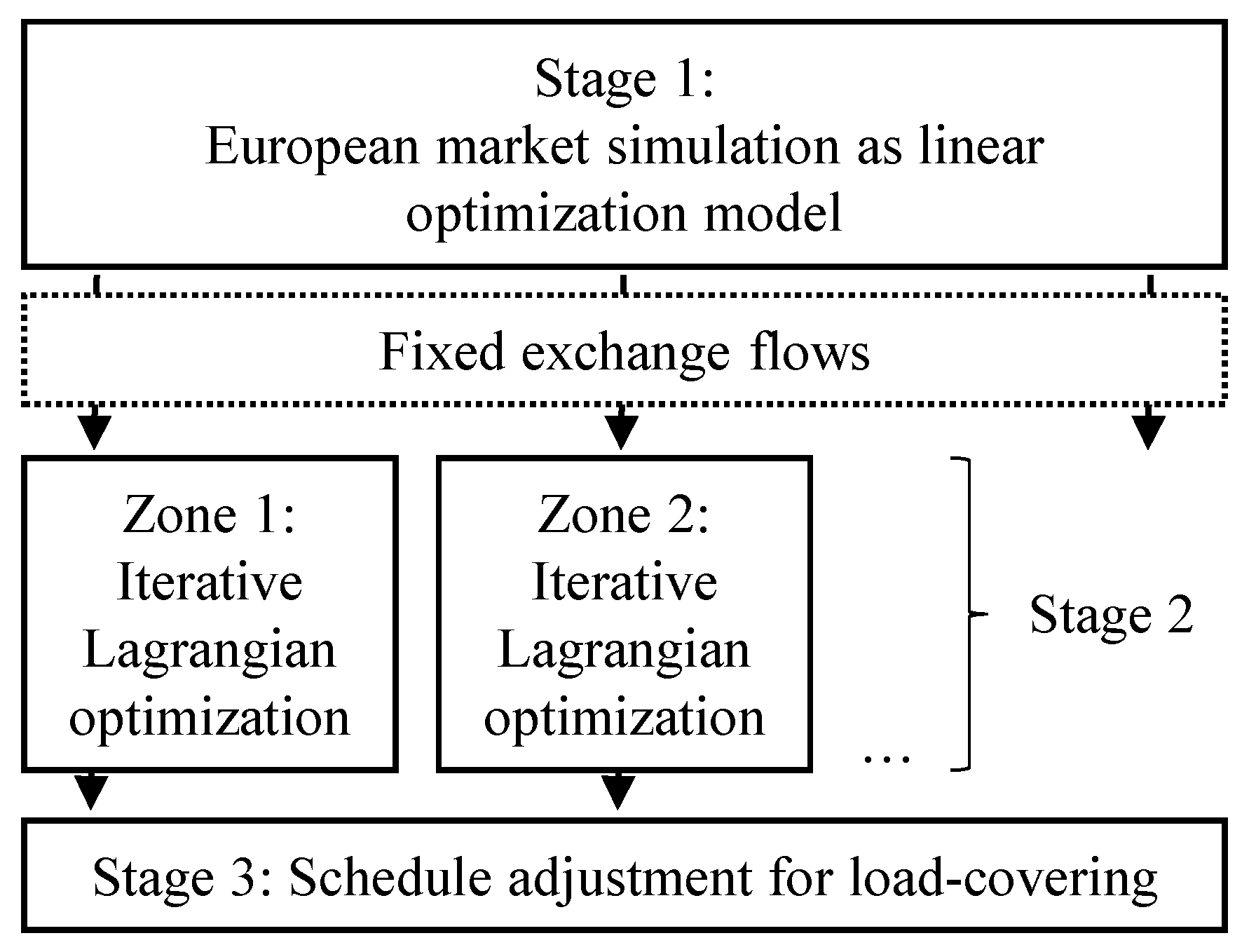
The multi-stage approach consists of two market simulations. The first stage focuses on the market coupling, including all market areas M but neglecting the detailed operational constraints of generation units. The second stage uses the market coupling outcome as a fixed input parameter and simulates a unit commitment of generation units within the market area.

The first stage is usually formulated as a linear optimization problem that minimizes operational costs $c_k$ of all generation units K within the simulation period T as in (1). Due to linearity, only a few constraints can be considered, e.g., a limitation of the power output between zero and the maximum output $\overline{P}$ as in (2) and a limitation of the ramping gradient of thermal power plants between $P_{\downarrow }$ and $P_{\uparrow }$ as in (3):

$$\begin{array}{ccccc}\hfill & \hfill & \hfill \underset{p}{min}\sum _{t\in T}\sum _{k\in K}{c}_k{p}_{k,t}& ,p\in {\mathbb{R}}^{+}\hfill & \hfill \end{array}$$

(1)

$$\begin{array}{cccc}\hfill s.t.& \hfill & \hfill 0\le p_{k,t}\le {\overline{P}}_k,& \forall k\in K,t\in T\hfill \end{array}$$

(2)

$$\begin{array}{cccc}\hfill & \hfill & \hfill P_{\downarrow }\le p_{k,t}-p_{k,t-1}\le P_{\uparrow },& \forall k\in K,t=2,\dots ,T\hfill \end{array}$$

(3)

The electrical load $D_m^{el}$ of each market area $m\in M$ must be covered in each time step $t\in T$:

$$\begin{array}{cc}\hfill D_{m,t}^{el}=\sum _{k\in K_m}{P}_{k,t}+N{P}_{m,t};& \forall m,n\in M,t\in T\hfill \end{array}$$

(4)

This constraint implies that the delta of the electrical load and the sum of the feed-in of generation units k must be balanced by the net position $N{P}_m$ of the respective market areas.

The net position can also be expressed as the sum of export flows $F_{m,n}$ minus the sum of import flows $F_{n,m}$:

$$\begin{array}{cc}\hfill N{P}_{m,t}=\sum _{n\in M}{F}_{m,n}-F_{n,m};& \forall m,n\in M,t\in T\hfill \end{array}$$

(5)

Market optimization is based on the idea of the endogenous optimization of net positions. Market coupling must be limited due to the constraints of the transmission grid. Therefore, two different approaches exist. In the NTC approach, exchange flows are limited by net transfer capacities ($NT{C}_{n,m}$) through (6):

$$\begin{array}{cc}\hfill 0\le F_{m,n,t}\le NT{C}_{m,n,t},& \forall m,n\in M,t\in T\hfill \end{array}$$

(6)

As a consequence, in the NTC approach, the electricity exchange can only be limited by bilateral constraints.

Another approach is defined by FBMC. In contrast to the NTC approach where only the exchange between two market areas is considered, net positions $NP$ are restricted by considering the impact on individual grid elements which are called critical network element and contingencies (CNECs) by linear sensitivities given by zonal power transfer distribution factors (zPTDF) $zPTDF$:

$$\begin{array}{cc}\hfill 0\le \sum _{m\in M}N{P}_{m,t}\ast zPTD{F}_{l,m,t}\le RA{M}_{l,t},& \forall l\in Lt\in T\hfill \end{array}$$

(7)

The remaining available margin $RA{M}_l$ represents the electrical capacity for exchange on the grid element l. The calculation method for $RAM$ can be found in [24].

The resulting net positions serve as fixed input for the second stage. For each market area, a detailed optimization problem for the dispatch of generation units is formulated. In addition, non-linear constraints of the operation can be considered at this stage [25]. This leads to a mixed-integer linear problem. These complex problems are often solved by decomposition approaches, in particular by Lagrangian relaxation.

The idea of the Lagrangian approach is to relax a complex constraint by penalizing the violation of this constraint in the objective function. Usually, in these cases, the load covering constraint is eliminated by this method. This allows solving the subproblems of generation and storage units separately. The respective multiplier is referred to as ${\lambda }_m$:

$$\begin{array}{c}\hfill \underset{{\lambda }_m}{max}\left\{\underset{P}{min}\sum _{t\in T}\sum _{k\in K_m}{c}_{k,t}+\sum _{t\in T}{\lambda }_i(D_{m,t}^{el}-P_{k,t})\right\}\end{array}$$

(8)

The optimal value for ${\lambda }_m$ is equal to the dual variable of the respective constraint and therefore, specifies the marginal costs for load covering which can be interpreted as the electricity price. The optimal value of ${\lambda }_m$ can be determined in an iterative process. It serves as a price incentive within the optimization of unit-specific subproblems. Therefore, the goal is to find a ${\lambda }_m$ which balances supply and demand. In the case of an overdemand, ${\lambda }_m$ will be increased and in case of an oversupply, it will be lowered. This process is repeated as long as deviations are minimized. The remaining deviations caused by binary on-/off-decisions by power plants can be eliminated in a third stage.

The whole process of the multi-stage approach is shown in Figure 1.

Using this approach, electricity prices are usually derived from the Lagrangian multipliers. However, there is no interaction between market coupling and the multipliers. This implies that the resulting market prices cannot be compared with each other. For example, exports from the more expensive to the cheaper market area may transpire.

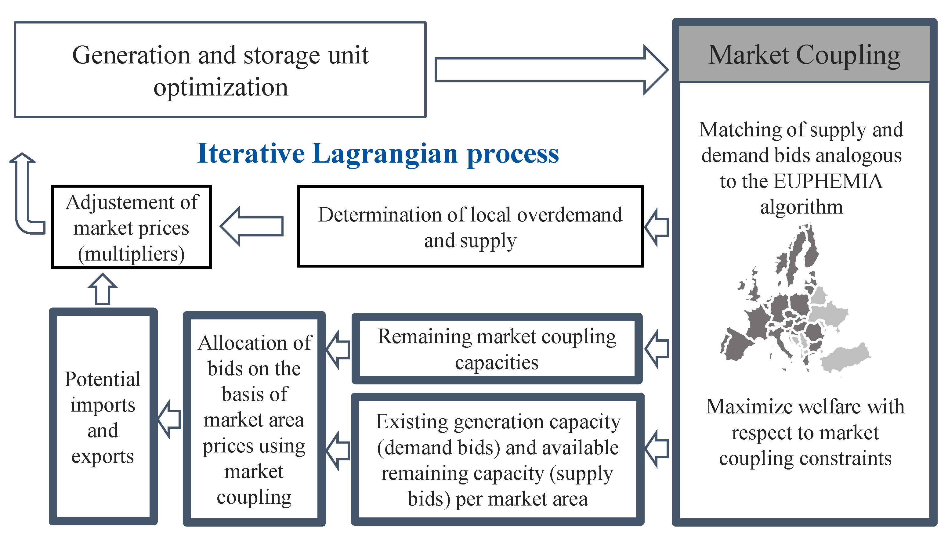
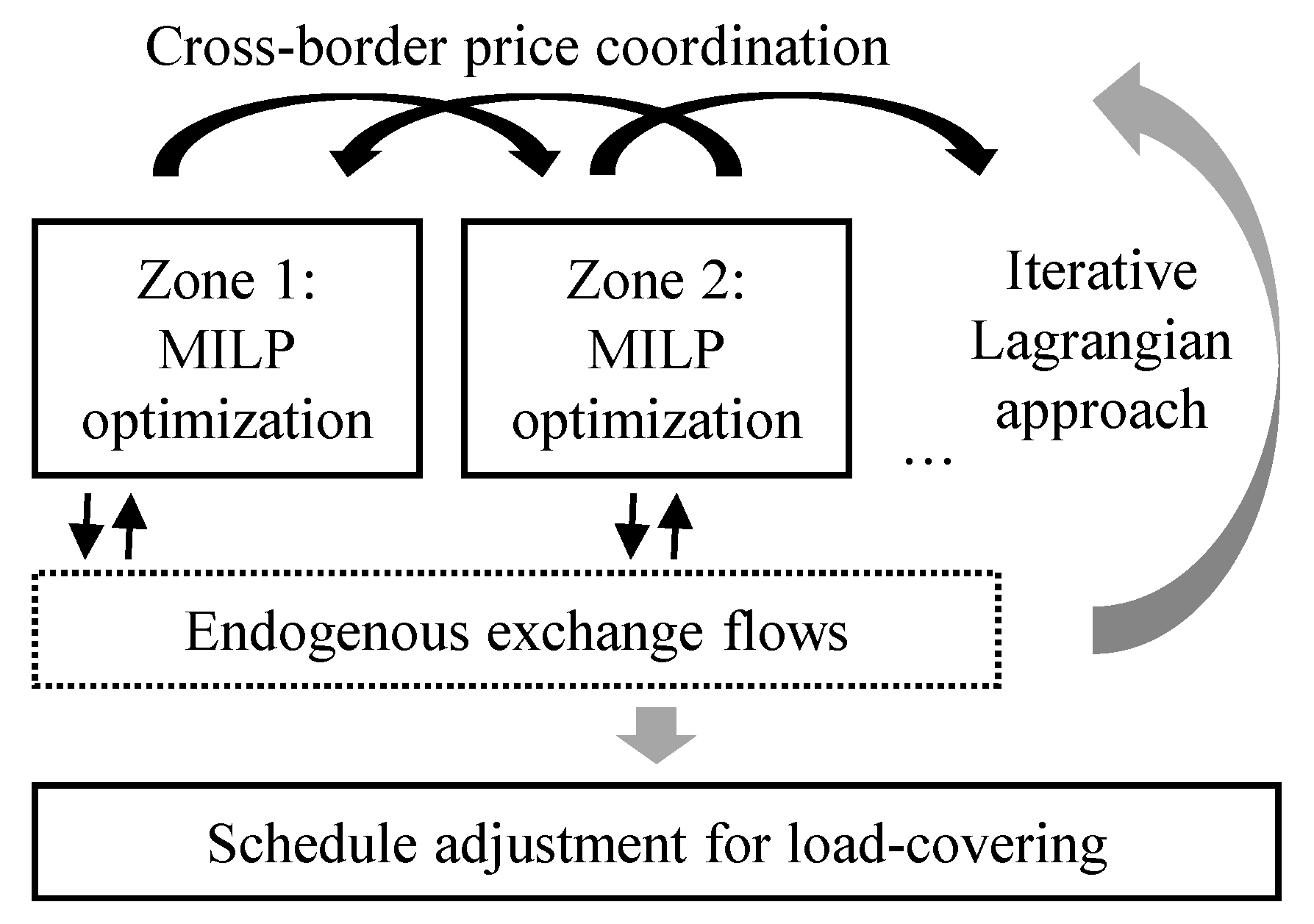
A method to overcome this problem is given in [15] using a single-stage approach, named European Lagrangian relaxation (EULR). The method is also based on Lagrangian relaxation. However, this approach uses multipliers for each market area interacting with each other. Therefore, prices are consistent with the market coupling outcome. Thus, the price adjustment process not only considers the deviation of load covering, but also potential imports and exports to align prices if exchange capacity is available.

The used decomposition includes all the subproblems of all market participants. The objective functions as in (8) are added with individual multipliers. The respective multiplier for each market area gives price incentives. All market participants optimize their operation against the given price incentive. The resulting bids are matched in a market coupling process analogous to the EUPHEMIA algorithm. The process is shown in Figure 2.

Similarly to the Lagrangian decomposition in the single-stage approach, Lagrangian multipliers are adjusted in an iterative process. The advantage of the single-stage approach is the accuracy of market coupling as it can be determined using mixed-integer linear programming (MILP) constraints within subproblems of generation and storage units. In contrast, in the multi-stage approach, operational schedules can change after the determination of market coupling.

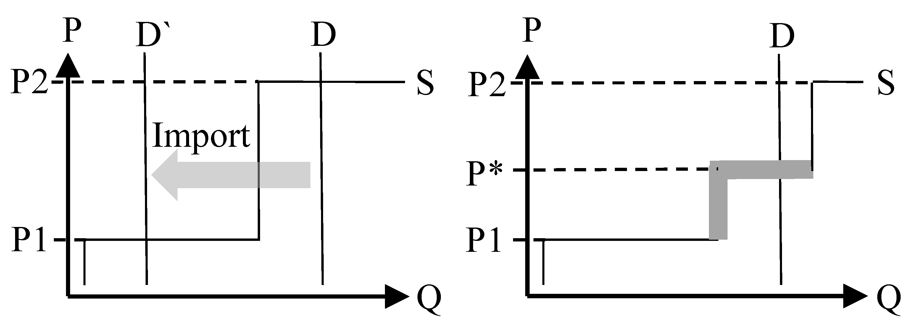
The problem concerning the price determination of the multi-stage approach is that prices are not simultaneously determined with the market coupling process. The underlying exchange flows do not reflect all operational constraints. However, as is the case with the actual flows, prices cannot be correctly determined if the price determination is in a subsequent step. This is caused by the fact that in market clearing, only supply and demand bids limited to the respective market are matched. Prices between the bidding prices of one market cannot result. This is demonstrated by Figure 3. In this example, inelastic demand is assumed. The left diagram illustrates an exemplary outcome of the multi-stage approach with only two supply bids and an exogenously considered import, resulting in the market clearing price P1. On the right, the full consideration of all bids within the multi-stage approach is demonstrated. This results in an actual market clearing price (P*) between P1 and P2.

This example shows that only a full consideration of market coupling leads to correct prices. To determine prices within a single-stage approach with Lagrangian multipliers, criteria for a price convergent state of the market must be defined. In a market optimal situation, the following can be applied:

1.

All supply bids with a price lower than the MCP and all demand bids with a willingness to pay higher than the MCP must be accepted within a market area. Note that the price of supply bids reflects the marginal costs in a competitive market;

2.

No exchange capacity can be left between market areas with price differences. This means that price differences can only occur if the exchange capacity is fully exceeded.

As a consequence, Lagrangian multipliers have to be adjusted in such a way that both criteria are met. The first criterion also exists in a single-market Lagrangian approach. To fulfill this criterion, the deviation between bidding quantities and quantities accepted in market clearing have to be determined. If not all demand bids are accepted, there is a local overdemand; vice versa, if not all supply bids are accepted, there is a local oversupply. Thus, for a single-market optimization, a Lagrangian multiplier that minimizes local overdemand and local oversupply has to be found. In a cross-market optimization, imports and exports must also be considered. If there are price differences and remaining exchange capacity, there is an import and export potential to increase welfare. To find optimal Lagrangian multipliers, these import and export potentials must be determined for each market area. Potential imports can be seen as further oversupply and potential exports as further overdemand.

The optimal Lagrangian multipliers can be determined by iterative adjustments. In each iteration, previous Lagrangian multipliers are adjusted based on the total overdemand and oversupply. The total overdemand indicates a need for an increase in the multiplier, the total oversupply a decrease in the multiplier. Assuming a continuous supply and demand curve, this iterative process has to be carried out as long as total overdemand and oversupply exist. Since demand and supply bids have quantities larger than zero with a constant price, their curves are non-continuous, and usually, total overdemand and total oversupply cannot be zero. Thus, the challenge is to find Lagrangian multipliers which minimize total overdemand and oversupply for each market area.

In each step of this iterative Lagrangian update process, local overdemand and supply as well as potential imports and exports must be determined. Whilst the identification of local overdemand and supply is independent of the applied market coupling procedure, the amount of potential imports and exports is limited by the constraints of the market coupling procedure.

3. Application in NTC and FBMC Approach

Two different market coupling procedures can be applied within a market simulation:

• The NTC approach considers the direct exchange between two market areas. The exchange on one link is independent of other links and thus completely neglects interdependencies through physical flows;
• Within the FBMC approach, bilateral exchange is handled ambiguously. Instead, net positions are optimized.

In the NTC case, criteria for price convergence can be applied by only considering the utilization of the exchange capacity of the respective link. The free capacity can be interpreted as the export potential of the market area with a lower price and the import potential of the market area with a higher price. In contrast, in the FBMC approach, free capacity cannot be assigned to specific market area borders. Consequently, criteria for price convergence must be applied to the overall market.

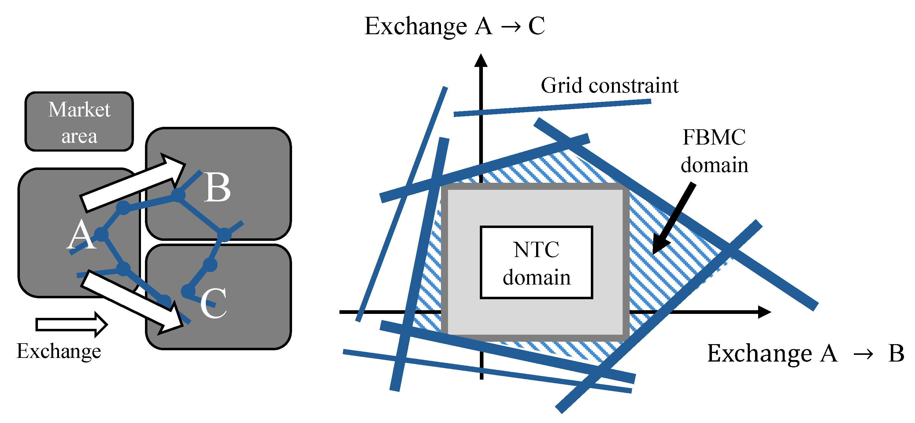
The theoretical difference between both approaches can be illustrated by a simplified example with three market areas A, B and C, as shown in Figure 4.

Using the NTC approach, the exchange from A to B and A to C is independent and results in the gray domain. FBMC considers the impact of the combined exchanges on the critical grid elements resulting in the blue domain.

The larger domain of FBMC enables the more efficient use of exchange capacity by ensuring the N-1 security of the transmission grid [26]. Therefore, welfare gains are possible [27,28]. Another flexibility of the FBMC approach that leads to welfare gains is that exchanges from the higher-priced to the lower-priced sector are possible within the FBMC approach. This flexibility can be used to enable a higher capacity for other exchanges that are constrained by the same grid elements. This phenomenon is called counterintuitive flow and is applied with the start of the flow-based plain [22]. In the previous flow-based intuitive, this was prevented by a constraint on the price-coupling algorithm [29].

Consequently, the calculation of free capacity as in the NTC approach is not applicable for FBMC. Therefore, the potential imports and exports have to be determined differently. The matching of potential imports and exports can be determined using the market coupling algorithm. The exchange capacities still available are considered for this purpose. This includes NTC capacities as well as FBMC capacities.

$$\begin{array}{cc}\hfill NT{C}_{m,n,t}^{avail}=NT{C}_{m,n,t}-F_{m,n,t},& \forall m,n\in M,t\in T\hfill \end{array}$$

(9)

$$\begin{array}{cc}\hfill RA{M}_{l,t}^{avail}=RA{M}_{l,t}-\sum _{m\in M}N{P}_m\ast zPTD{F}_{m,l,t},& \forall t\in T\hfill \end{array}$$

(10)

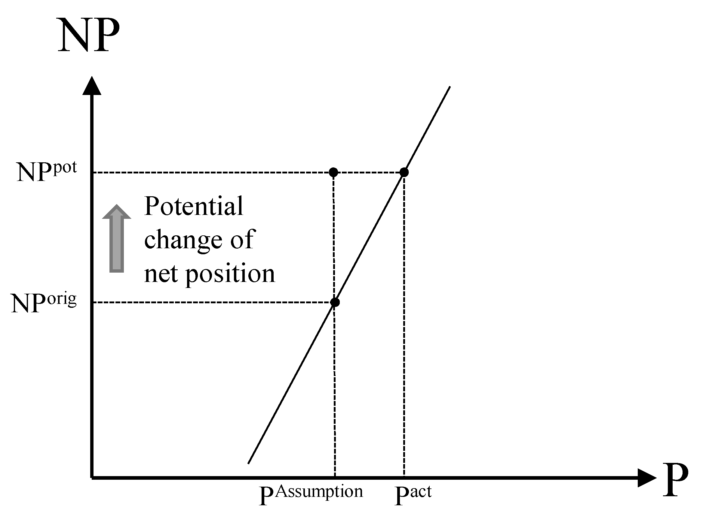
For the application of the market coupling algorithm analogous to the EUPHEMIA algorithm, relevant generation and demand for the import and export of each market area have to be put into the form of price–quantity bids. To smoothen price differences, the generation of high-price areas should be replaced by the generation of low-price areas. Consequently, the current generation that can potentially be substituted should be interpreted as demand, while unused generation capacity can be interpreted as supply. As long as the change in the net position of a market area is small, price steps within the supply and demand curves resulting from different marginal costs and utility can be neglected. Thus, the current market price within the iteration can be used as the price of an additional export or import. The relationship between the change in net position and the price with the assumption used is shown in Figure 5.

Under this assumption, the potential import and export can be calculated per hour by the optimization of:

$$\begin{array}{cc}\hfill mi{n}_p\sum _m{c}_m{p}_m^{avail}-c_m{p}_m^{act}& ,p\in {\mathbb{R}}^{+}\hfill \end{array}$$

(11)

This objective function is analogous to (6) and (7) subject to:

$$\begin{array}{cc}\hfill 0\le F_{m,n,t}\le NT{C}_{m,n,t}^{avail},& \forall m,n\in M,t\in T\hfill \end{array}$$

(12)

$$\begin{array}{cc}\hfill 0\le \sum _{m\in M}N{P}_{m,t}\ast zPTD{F}_{l,m,t}\le RA{M}_{l,t}^{avail},& \forall l\in L,t\in T\hfill \end{array}$$

(13)

The resulting exchange flows indicate potential imports and exports. Those can be seen as additional oversupply and overdemand similar to [15]. Thus, the total oversupply consists of the actual oversupply and the potential import. The total overdemand consists of the actual overdemand and the potential export. In the subproblem optimization of the next iteration, the price incentive in the case of oversupply is lower whereas the total overdemand must lead to higher price incentives. This iterative process is repeated as long as all convergence criteria are met. This process is illustrated in Figure 6.

4. Simulated Electricity Prices

The discussed concepts are evaluated using two different scenarios. At first, a backtest for 2014 is carried out to prove the precision of the single-stage approach and its advantage compared to the multi-stage approach. Subsequently, a future scenario for the year 2035 is analyzed.

4.1. Backtest Results

The backtest validates the discussed approaches by comparing their resulting prices with real prices for the year 2014 with a focus on Germany. The respective electricity day-ahead prices are shown in Figure 7.

For the backtest simulation, a historical scenario framework of the European electricity market of the year 2014 was used. This framework consists of generation, storage and exchange capacities as well as renewable feed-in and demand time series. Moreover, historical fuel and CO${}_2$ prices were applied. A full description of the scenario assumptions can be found in [15]. Since the FBMC was not applied in 2014, the market is coupled via NTC. The results of this simulation show high similarity between the simulated generation schedules and the historical schedules [15]. This results in a close approximation of price levels. The mean price is EUR 0.51/MWh which is lower than the historical price for Germany, and can be explained by the assumption of perfect foresight. Figure 8 shows the respective price distribution.

The same simulation framework is applied to the multi-stage approach. For the first stage, the approach provides a pan-European view, neglecting detailed restrictions to determine exchange schedules. To prevent price differences resulting only from exchange deviations, the resulting exchange schedules of the EULR approach are applied to the second stage. In this stage, detailed generation schedules and electricity prices that result from the endogenously given exchange for each market area are calculated. In sum, generation quantities do not differ significantly [15]. Prices, however, differ overall, as indicated by the price distribution shown in Figure 9.

It can be observed that the prices in Figure 8 are more homogeneous and their distribution is smoother. In contrast, prices in the single-stage approach are more concentrated. This results from the fact that the price bids of neighboring market areas do not affect the merit order of the focus area in the second stage. Since the exchange is exogenously included, the foreign bids cannot influence the price. Instead, the assumed export and import flows are considered price-neutral. In this case, this leads to a decrease in the average price by EUR 2.77/MWh compared to the historical price.

If the exchange schedules resulting from the first stage are applied to the second stage, the distortions in the price distribution increase. This is also caused by distortions in the exchange due to the application of market coupling with simplified power plant restrictions compared to [25] as in the EULR approach. The distribution curve is shown in Figure 10.

The backtest results show that the EULR approach leads to the most realistic price distribution and can determine precise market prices. On the one hand, the correct calculation of exchange flows is essential with the full consideration of relevant constraints. On the other hand, the market coupling should be respected in the market clearing for the price determination. For future simulations, the future regulatory framework must be considered. The applied FBMC imposes special requirements on price determination. These differences are analyzed in the following paragraph.

4.2. Impact of FBMC and NTC

For investigating the impact of the FBMC approach compared to the NTC approach, a future scenario for the year 2035 is simulated. The scenario framework is described in [30]. In this scenario, FBMC is applied to the CORE region according to [31]. The regulatory framework includes the application of advanced hybrid market coupling and the possibility of counterintuitive flows [32]. To give an example of different effects between electricity exchange flows and prices in FBMC compared to the NTC approach, the HVDC connection ‘ALEGrO’ between Belgium and Germany is depicted. This HVDC line connected via the evolved flow-based market coupling was chosen as an example because the commercial exchange flow matches the physical line flow and can be clearly determined in contrast to other connections based on AC interconnectors. Within the NTC approach, only intuitive flows are possible. This means that Belgium exports to Germany if the price in Germany is higher than in Belgium, and Belgium imports from Germany in the opposite scenario. For a full year simulation, this results in the following aggregated flows illustrated in Figure 11.

In contrast, in the FBMC approach, counterintuitive flows are also possible. This means that the commercial flows do not strictly follow the rule of a flow from the lower-price market area to the higher-price market area. The reason for this is that different exchanges are affected by the same limiting grid elements. In this particular case, a physical interconnector line between Belgium and France has significant influence. The respective CNEC has a strong positive sensitivity to exchange flows from Germany to Belgium and also a strong sensitivity to the exchange from Belgium to France. This CNEC limits the CORE FBMC to several hours, which can be seen in Figure 12.

These additional exchange restrictions are accompanied by a higher electricity price gap since a full utilization of the exchange capacity can only exist with a price gap in both cases. This is shown by the annual duration curve of the price gap in Figure 13.

The mean absolute price gap between Belgium and France in the FBMC approach is EUR 6.20/MWh whereas the price gap in the NTC approach is EUR 3.34/MWh.

Exchange flows from France to Belgium can be compensated by flows via ALEGrO from Belgium to Germany in specific cases. These counterintuitive flows occur in 436 h in the annual simulation. In 433 h, there is a commercial flow from Germany to Belgium although the price in Germany is higher than in Belgium and in 3 h in the opposite scenario.

Price gaps and counterintuitive flows are more likely in winter due to high absolute price peaks driven by a high residual load. An exemplary situation for a counterintuitive flow is given in hour 33 of the annual simulation. In this case, there is a generation surplus in France due to high nuclear generation, whereas Germany imports due to low renewable feed-in. This is illustrated in Figure 14 and Figure 15.

The flow from Germany to Belgium can increase exports from France. In this case, the interconnector between Belgium and France is restrictive for the market coupling. The flow via ALEGrO lowers the approximated load on the respective CNEC. Therefore, it contributes to the increase in market welfare which is not apparent from a consideration of Belgium and Germany only. This situation is illustrated in Figure 16.

These results exemplify how counterintuitive flows can occur in the European electricity market. From an overall perspective, this can increase the total welfare of the European electricity market. Since the maximization of total welfare is the objective of market clearing, this must be taken into account for the price determination.

5. Discussion

The determination of electricity prices by fundamental unit commitment models in large-scale coupled electricity markets such as the European market is challenging. Clearly, the accuracy of data and the precision of individual generation and storage models is essential. However, we could prove that the chosen approach influences the resulting prices. The single-stage approach which is presented in this paper allows for realistic prices, as shown in the backtesting. The concept of this approach can also be applied to future scenarios including regulatory adjustments to market coupling. Historical parallel run results of flow-based plain in CWE show that significant price differences associated with welfare gains are possible compared to the flow-based intuitive [29]. The effects of the actual changes have so far only been empirically studied to a limited extent due to the finite time of application. Moreover, external effects, especially the COVID-19-crisis, have significantly influenced the market [33]. Additionally, the current increase in minimum exchange capacity until 2025, following the Clean Energy Package of the EU [34], will lead to enhanced price convergence. Therefore, a conclusive empirical comparison of the effects implied by flow-based plain and the evolved flow-based plain is hardly possible at present and should be assessed in the future. However, there are limitations for the price determination resulting from modeling assumptions. In the scenarios of the case studies, no distinction is made between future and spot markets, nor between day-ahead and intraday markets. This implies that exchange capacities are optimally used as no long-term nominations exist and there is an optimal generation and storage dispatch as perfect foresight is assumed. Both can result in higher temporal and cross-market price gaps which cannot be replicated with the model.

6. Conclusions and Outlook

The determination of electricity prices using fundamental market simulations is of great interest for the assessment of future scenarios. The introduced single-stage approach in this paper improves the modeling of price determination compared to frequently used multi-stage approaches. Both approaches ordinarily use a Lagrangian relaxation. The advantage of the single-stage approach is that it allows for optimizing market coupling as well as generation and storage operation simultaneously and thus taking into account the price information of neighboring market zones. Distortions in electricity prices that would otherwise necessarily occur are avoided. However, the single-stage approach requires a more complex iterative adjustment process of the Lagrangian multipliers to determine a convergent solution that reflects the optimum. Thereby, the specifications of the respective market coupling approach, either NTC or FBMC, must be taken into account in order to ensure correct price differences between the market areas. Whereas for the NTC approach a bilateral consideration of exchange is sufficient, price adjustments within the FBMC approach are only possible regarding the overall market if counterintuitive flows are possible. In the exemplary backtest for the German electricity spot price for 2014, the single-stage approach achieved a more accurate price distribution than the multi-stage approach. In another case study, we have shown that the single-stage approach is also applicable for future scenarios using FBMC as a proof-of-concept. In the future, this approach can be further improved if respective datasets for further backtesting are available. Considering uncertainties for market participants could increase the accuracy of price modeling, as demonstrated in [3]. Moreover, future regulatory changes regarding market design must also be considered. For example, the market integration of decentralized generation poses new challenges for price convergence [35].