1. Introduction
Electricity is at present indispensable. Electricity generation results in various environmental and social consequences depending on the type of fuel (e.g., coal, gas, etc.) used to produce the electricity. Environmental consequences are generally more severe when the electricity comes from non-renewable sources (e.g., fossil fuels), which produce a greater amount of emissions than renewable ones (e.g., wind and solar). The emissions affect regions that are even distant from the the electricity production site. This uncontained issue exacerbates climate change, introduces toxins into the atmosphere [
1], and generally contributes to many environmental injustices [
2].
There are several energy-management approaches in the literature that aim to reduce the emissions attributed to energy consumption. These approaches can be divided into two main categories: (1) enhance efficiency, and (2) optimally shift energy consumption (demand) in space and/or time. The former strategy involves improving the electrical instrument’s efficiency, such as investments in equipment and the electricity grid, which has direct interactions with emissions and economic performance of the region [
3]. For instance, investments on replacing five percent of the European hybrid transportation sector with Electric Vehicles (EVs) [
4], or obtaining LEED (Leadership in Energy and Environmental Design) and other green building certifications [
5]. This strategy is fulfilled through the use of efficiency-enhanced equipment, leading to less energy consumed per energy output and thereby less emission per energy output. Even though the payback would be quick, business owners are often reluctant to implement such improvements, which are often costly [
6]. The latter strategy relies on a Demand Response (DR) program, which incentivizes electricity consumers to properly time shift their daily load profile away from times of high emissive generation to times of lower emissive generation (e.g., switching from coal-fired to solar powered generation). Presently, various DR programs are being adopted by grid operators to balance the supply and power demand as they wish. These programs can potentially lower the cost of electricity production in the wholesale market, and consequently, reduce the retail rates. The electric power utilities consider DR programs to be valuable resources because of their lucrative benefits such as their potential in positively impacting the grid modernization and optimization. Electricity consumers can respond to a DR program by either actually shifting their time of energy use or employing energy storage systems such as batteries [
7,
8] during times of high electricity emissions. In Michigan in the United States (US), nearly half of the electricity comes from coal power plants, which produce the highest amount of air emissions compared with the other types of Electricity Generation Units (EGUs) [
9]. Displacing this type of generation technology with “green” energy sources will result in a considerable improvement in public health and environment.
Many researchers have investigated and pointed out the social, environmental, and public health-related advantages of replacing conventional energy sources with more environmentally friendly ones. For instance, Siler-Evans et al. [
10] provided important estimates of the health, environmental, and climate benefits from investing in wind and solar energy sources instead of conventional pollution-intensive power plants. Their approach relied on the use of the historical data of the emissions associated with electricity generation in the US.
The Siler-Evans approach was then modified and improved by (Thind et al., (2017)) [
11], which focused on estimating the Emission Factors (EFs), Average Emission Factors (AEFs), and how they are different from Average Marginal Emission Factors (AMEFs) for the Midcontinent Independent System Operator (MISO) region before and after its geographic expansion footprint in 2013.
Unlike the aforementioned research efforts, which depend on the use of historical data, the Locational Emission Estimation Methodology (LEEM) [
12] model calculates the emission factors based on available real-time data of the power grid. Real-Time techniques mostly rely on the information reported from each Commercial Pricing Node (CPN). The information includes the demand, electricity generation, and price. These models then predict the fuel type and estimate the associated emissions based on the fuel type and electricity generation technology. LEEM takes the Locational Marginal Price (LMP) information from the US Energy Information Administration (EIA) and estimates the air emission (lb/MWh) based on the combination of fuel types and the prime movers of each of the locations. In general, there can be up to 39 types of fuel and 17 types of prime movers, resulting in 116 combinations of prime movers and fuel types in total. This large number demonstrates the degree of the complexity possessed by the LEEM approach. Although the model was originally developed for the MISO region, it is applicable to any other LMP-based electricity market [
13], such as PJM, CAISO, and NYISO. The very last version of LEEM has been successfully tested to be able to estimate the emissions associated with electricity production at any time and node of a power grid. [
14]. Unlike the previously developed methods, in LEEM the emission reports are calculated based upon five-minute real-time specific emission factors, which vary over time and location. It should be mentioned that LEEM is geographically sensitive and reports historical, real-time, and day-ahead detailed data for each location, that is, distinct from prior approaches, it is not limited to an average report for a region. Moreover, the historical approaches suffer from a key limitation; they rely on historical and past relationships, which prevent them from modeling the future grid operation and MEF estimations which might differ from those of the past. The outcomes of this improper emission estimation tool can potentially assist with reducing emissions without limiting the electricity consumption if implemented in innovative decision-making tools. By having the insights about estimated emissions, one can appropriately time shift the electricity demand to reduce the peak load on the electric grid when the electricity is being generated from non-green fuel resources [
15]. This load shifting eventually leads to environmental and grid management benefits. Water industries are one of the best electricity customers to apply the load shift because of the available flexibility through pumping schedules, storage capacities, and utilizing on-site generations. Zohrabian and Sanders (2021) [
16] recently tested the strategical electricity load management by shifting 5% of the daily electricity demand of water industries to the times with the lowest emissions (i.e., cleaner fuel resources) in the California Independent System Operator (CAISO), which resulted in a 2 to 5% annual CO
2 emission reduction.
The LEEM model was adopted in numerous applications such as Home Emissions Read-Out (HERO) [
17], energy optimization tools applied to real-life water networks in Monroe [
18], and reducing electricity usage cost and the associated pollution emissions of water pumps within water distribution systems by introducing a Pollution Emission Pump Station Optimization tool (PEPSO) [
19]. Although Rogers et al., (2013) [
14] performed various analyses to improve and evaluate the reliability of LEEM through power system simulations, suggesting that LEEM provides a means of incorporating pollutant emissions into demand side decisions, there has not been any attempt to compare LEEM with the historical-data-oriented approaches. This comparison will make the use of LEEM data applicable to Wayne State University (WSU) campus as a case study. The authors developed an Electricity Emission Factor dashboard in 2018 [
20], which will be used for this purpose. This study includes both numerical and temporal comparisons between LEEM and two other approaches from the literature [
10,
11]. The studies are focused on the same scope and area, but they use different methodologies.
2. Background
The Emission factor (EF) is a ratio that denotes the normalized emissions attributed to the use of electricity at a specific location and time in unit of pollutant weight per one kWh of generated electricity [
21]. Conversely, the Marginal Emission Factor (MEF) estimates the amount of the emission per kWh that would be realized at a specific time and location if one additional unit of load were placed on the power grid at that specific time and location. In other words, the MEF of a grid node is the total amount of additional emission that would be generated if one additional unit of load were placed at the same node of the grid. MEFs provide a consistent metric to achieve a spatial and temporal representation of how clean or polluted a power grid is [
21].
There are different approaches to calculating the Emission Factors (EFs). Some of them calculate the average EFs on a regional basis and some others provide temporally varying estimates. Unlike LEEM, the basic approaches [
10,
11,
22] present the ratio between the total emissions released into the atmosphere and the total electricity generated using the historical data provided by the EPA Continuous Emissions Monitoring Systems (CEMS) [
23], whose data resolution is within hourly time intervals. There also are some other approaches that model a series of factors, known as Average Marginal Emission Factors (AMEFs), based on bid-dispatch simulations of electricity generators, predicting which type of electricity generation unit is on the margin and if the total energy demand at that time will increase. These approaches use Locational Marginal Price (LMP) released by the Independent System Operator (ISO) based on the bids and offers between energy generation companies and load-serving entities. LMPs are publicly available. They are reported by the US EPA Energy Information Administration (EIA) [
24] on a real-time basis. LMP is the system minimum cost to satisfy one additional megawatt of electricity demand at a specific time and location [
25].
The LEEM model uses the Locational Marginal Price (LMP) approach, which is quite different from Siler-Evans et al. and Thind et al. These authors [
10,
11] adopt the historical observations reported by CEMS to predict the short term EFs and MEFs. The LEEM model uses the same database but derives the MEFs from LMPs and different fuel combinations, to represent the emissions in two different ways, one based on the highest probability and the other is based on weighted probability. The highest probability approach returns the MEF values associated with the most probable fuel and generation types using LEEM’s stochastic approach. On the other hand, the weighted approach uses the full probabilistic distribution, with appropriate weighting, to return the weighted MEF that takes into consideration the full range of probabilities. Both of the two approaches rely on LEEM’s use of LMPs and power systems’ data.
LEEM employs a stochastic approach for estimating the real-time MEFs on a five-minute basis at 182 Commercial Pricing Nodes (CPNs) within the state of Michigan, demonstrating a finely spatial variation. One of the unique features of LEEM is its precise geographic and detailed time reports of emission estimations. The local regions in LEEM are defined by the US EPA’s Emissions and Generation Resource Integrated Database (eGRID) Subregions [
26], which is the same as the definition adopted by the North American Electric Reliability Corporation (NERC) [
27].
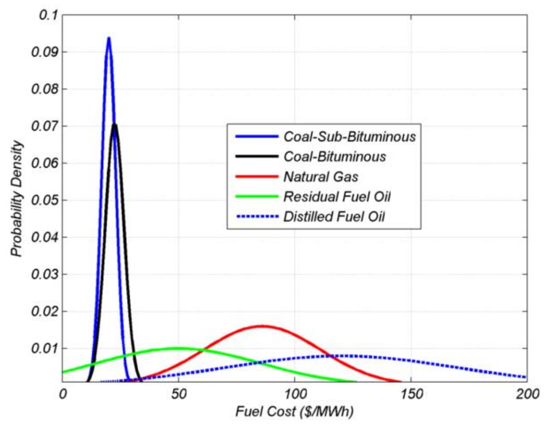
The EIA-923 form provides the primary fuel type (e.g., coal, natural gas, or petroleum) for each power plant, which is in accordance with the three fuel types defined in LEEM. In many cases, the EIA-923 reports are on a specific fuel type, such as sub-bituminous or bituminous coal. Instead, in LEEM, an alternative approach is employed, which utilizes the probability density curves of plant fuel prices so as to more accurately identify LMP price ranges.
Figure 1 shows the normal probability density curves created for each fuel type based on the data of the eGRID subregion RFCM.
LEEM utilizes average regional emission rates of specific power plants reported in the latest version of eGRID (eGRID. 2018). Emission rates at each plant for CO
2, SO
2, and NO
X equivalents are reported in pounds of pollutant per megawatt-hour of generated electricity (lb/MWh). Carbon dioxide equivalents are calculated based on the global warming potential of CO
2, CH
4, and N
2O [
28]. Average emission rates and standard deviations are calculated for each fuel type and pollutant, accounting for all plants in the region. The average emission rates are also weighted based on the amount of electricity produced at each power plant (weighted probability) besides reporting the highest probable fuel type and the source power plant. In order to improve the accuracy of the emission estimation, a Membership Function (MF) is assigned to LEEM which considers all the marginal generators. Aiming to increase the likelihood of characterizing the fuel mixture of marginal units, the MF variable is derived from Fuzzy Logic by Rogers et al. [
17].
There are some similarities between LEEM and those developed in prior studies [
10,
11]: firstly, Thind et al. [
11] and LEEM both use an RTO (Regional Transmission Organization) framework which provides a better representation of electricity dispatch than the NERC (North American Electricity Reliability Corporation) approach considered by Siler-Evans [
10]. Secondly, Thind et al. [
11] and LEEM both use total MISO generation and account for all available fuel types, generators, and fuel combinations. The Siler-Evans study [
10] accounts for only fossil fuels. Finally, it can be said that the Thind et al. study calculates both AEFs and AMEFs, whereas LEEM reports the real-time MEFs by predicting them on a day-ahead basis.
Therefore, this study is focused on comparing LEEM with Thind et al. [
11] due to their similarities in source and scope, and also because Thind et al. is an improved version of a historical data approach, which was first developed by Siler-Evans [
10]. Then, for our second comparison, we use the data exported from Climate and Energy Decision Making (CEDM) in the program of Engineering and Public Policy at Carnegie Mellon University [
29]. CEDM uses a huge amount of raw pollution data for every fossil-fired power plant within the US that has a minimum capacity of 25 MW. Here by raw data, we mean the data that is being fed into LEEM. Hourly emissions are calculated by aggregating all exhaust pollutants of each of the power plants in that specific US EPA’s Emissions and Generation Resource Integrated Database (eGRID) subregion, and then pairing with the total electricity generation. The mentioned set is then linearly regressed such that the slope of the resultant line will give the MEF estimates. Thind et al. and Siler-Evans [
10,
11] used the same linear regression model to estimate the hourly AMEFs and MEFs as well as predicting the emissions for a short time ahead. The CEDM website provides the AEFs and AMEFs for all RTOs, sourced from the US EPA EIA data presented publicly and compared to LEEM data, which can be used to demonstrate the similarities and differences.
3. Materials and Methods
Here, we took advantage of comparing LEEM MEFs with the Thind et al. study [
11] as it includes the MEF estimations both for pre- and post-MISO geographical change in 2014 and also CEDM, which reports MEFs until 2019 for each year, so that we can better analyze the differences and similarities in the data and trends. MISO contains 15 Midwestern US states and serves nearly 42 M people (which makes up 13% of the US population) acting as an air traffic controller for the Midwest electric grid. MISO is operating one of the world’s largest energy markets with an annual market energy transaction of
$29 billion. Currently, MISO oversees a generation capacity of 147,000 MW (which makes up nearly 16% of the total US generation) and 65,800 miles of electricity transmission lines [
30,
31]. MISO experienced a geography change in 2014 and was called Midwest ISO before. This section discusses the basis of comparison between the LEEM, Thind et al., and CEDM approaches and their methodologies using the various marginal emission factor (MEF) estimation tools. In general, this discussion contrasts that LEEM employs a stochastic approach, defining the probability of different outcomes, and that the other studies [
10,
11] rely on a predictive model using historical data. There are some limitations in comparison areas which are defined below. The complications of this study are that the region under study not entirely but partly makes up that of the counterpart studies and that the time frames covered in this paper and the other studies do not fully match due to an unavailability of data and the fact that these studies were not developed in the same year. However, the aforesaid limitations do not discount the study overall since it is the trends from the data and system behaviors which are being compared.
3.1. Locational Limitations
In this study, the focus is on the LEEM emission estimation dataset reported for the closest transmission bus (CPN) to the WSU campus (Detroit, MI 48202, USA). Due to the differences in the regional scale of the various approaches (site-specific vs. regionally averaged), it seems impossible to compare the emission estimations for the same location. However, this study made comparisons as geographically consistent as possible by ensuring that the larger scale of the Thind et al. and CEDM application comprise the specific locations of the LEEM application. The LEEM method is applied to the geographic location of the College of Engineering at WSU in Detroit (Latitude: 42.355472, Longitude: −83.070724) while the other two methods provide the MEF for the ISO that includes this location, MISO. Of course, since the geographic locations being compared are not identical, we do not expect the specific comparisons to be “spot on”. However, the goal of the comparison is to point out the similarities and differences in the trends identified by the various methods, not the specific values. Therefore, the authors believe that the proposed approach is appropriate.
3.2. Temporal Limitations
The datasets from the paper of Thind et al. [
11] and CEDM [
23] cover different time periods than those from LEEM. The database of Thind et al. has nine years of data, and CEDM has three. LEEM, since it was launched in 2018, has collected only two years worth of data, but this data is on a five-minute basis at 182 CPN locations within the state of Michigan, demonstrating a finely spatial variation. The data available in [
11,
23] and LEEM is enough to show seasonal similarities or differences. Therefore, although the data for each study is not captured in the same timeframe, the expectation is that the emission intensity trends should be similar. This study provides different comparisons for the MEFs reported by Thind et al., CEDM, and LEEM. Other than the numerical comparisons between the different datasets, we also compare LEEM with the temporal trends in the emission factors reported by Thind et al. The comparison will be carried out over different time frames including yearly, monthly, daily, and even hourly.
Comparing emission intensity in various time frames highlights the differences between the Thind et al. study, which uses historical data observation, and the LEEM model, which uses a stochastic model calculating the emission intensity in real-time at any specific geographic location. To achieve more accurate outcomes, several different comparisons are required, especially temporal comparisons, because for the regions with variable diurnal or seasonal electricity demand, neglecting time variation will lead to unrealistic results. Typically, the regions with larger portions of hydro or wind in electricity mix have more emission variations [
32]. Some authors [
33] indicated that the marginal emission of an hour of a day may be up to twice as big as that of another hour of the same day. Thus it is imperative to perform different sets of comparisons with fine temporal granularities. Temporal comparison in MEFs has a critical role in this study because, despite the fact that MEFs vary over time and location, each RTO has a specific and logical time-tagged footprint. For instance, the emission intensities are usually higher when there is lower electricity demand, such as early mornings and late evenings when wind power is not present for the Midwest. We represent detailed comparisons whose time periods vary from annually to hourly, which is the finest available output from other models. It is important to note that LEEM, which estimates the emissions, performs a trend similar to that of the historical approaches. The advantages of LEEM over prior studies were already reviewed and will be discussed in the subsequent sections as well.
3.3. Annual Comparison
Because of the limited availability of the annual data and also the differences in the models, we use the equation below to define and calculate a relative index for comparative evaluations of Thind et al., (2007 to 2016), LEEM (2018–2019), and CEDM (2013–2017–2018).
where
D is the percent difference in the reported emissions, AMEF is the marginal emissions reported by Thind et al. and LEEM and
CMEF denotes the emission reported by CEDM. In our annual comparison, each year, if possible, is compared with the same year, and with its closest corresponding year if otherwise.
3.4. Monthly Comparison
When comparing the different approaches, which are providing similar results (MEFs) when the same data is fed into the models, it is imperative to include different time frames in the analysis of the trends of the reported data. Both the approaches we are considering here are reporting MEFs for the same power grid. However, the geographical scale is not the same. The focus of this study is on comparing the trends rather than the numbers because: firstly, the geographical studies do not have the same amount of area covered; secondly, the data resolution of the approaches are different. The LEEM reports are generated on a five-minute basis, whereas the reports of Thind et al. are generated hourly. Therefore, this study aims at considering the regional footprint and behavior during different time frames and investigates the similarity of the trends.
3.5. Daily Comparison
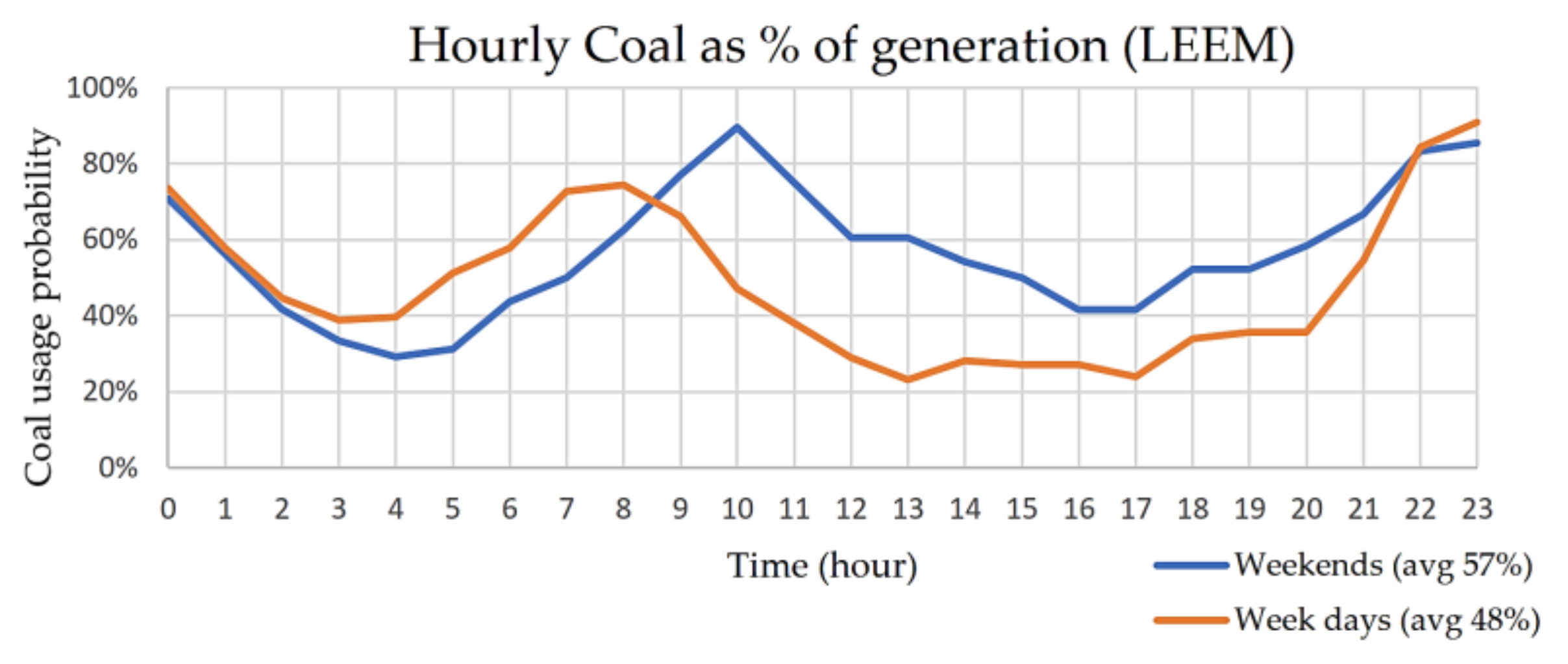
This study also looked at the differences between weekdays and weekends. Due to the reported differences within the study of Thind et al., it was interesting to see if the same trends are observed in the LEEM study. This comparison, in spite of data availability issues, is still relevant to show that power plants behaviors intend to use specific fuels on the margin. The daily comparison shows that the emission intensity is higher during the weekends.
3.6. Hourly Comparison
Comparing the LEEM MEFs dataset, including reports with five-minute intervals which are 12 times bigger than the historical MEFs dataset reported by Thind et al. in an hourly basis, demonstrates how close the daily trends recognized by LEEM are to the other historical methods. The historical data, for instance, highlight that the emission intensities are higher during early mornings and late evenings when the power demand is lower and renewable energy, such as wind and solar, are not operational.
4. Results
The following metrics have been chosen to evaluate and compare the LEEM approach with the existing approaches for MEF estimations, including CO2, SO2, and NOx. The LEEM method provides MEF estimations for Mercury and Lead, whereas the other approaches are not providing estimations for mercury and Lead. Thus, they are not discussed in this paper. This comparison is based on the historical data reported by LEEM for the closest commercial pricing node (CPN) to the WSU campus as a LEEM sample location, the emission data provided by Thind et al., (2017) study, and CEDM.
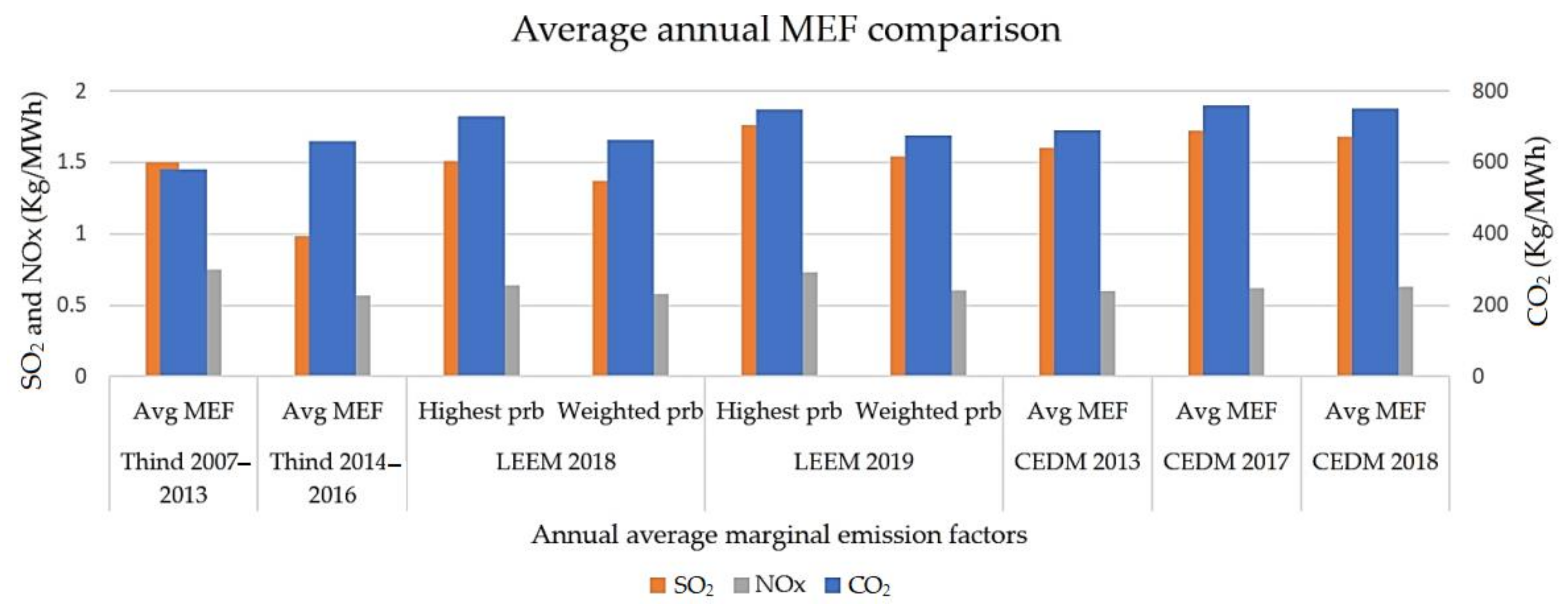
4.1. Annual MEFsCcomparison Results
Annual average data for all three studies are shown in
Figure 2. Data from the CEDM website is reported for 2013 (before MISO changed), 2017, and 2018. Our weighted results for 2018 and 2019 are closer to the website numbers (used as the reference because this historical data is reported by the EIA) reported for AMEFs rather than the numbers reported by Thind et al. for 2007–2013 and 2014–2016 (see
Table 1).
The LEEM values (weighted probability) are adopted to be compared with Thind et al. and CEDM values. We use weighted probability data because LEEM is so specific with very fine resolution on location, and therefore the Highest Probability may overestimate the peaks and underestimate the troughs since the methods targeted by the comparison use a more regional approach. The results demonstrate that the AMEFs are decreasing over time (years) after the MISO geographical change. As another finding in the annual comparison, it is seen that the numbers provided by Thind et al., for 2014 to 2016, are close to the weighted numbers obtained using LEEM data.
As
Table 1 shows, LEEM MEFs were closer to the data reported by the CEDM website for the annual averages and had a lower percentage of difference.
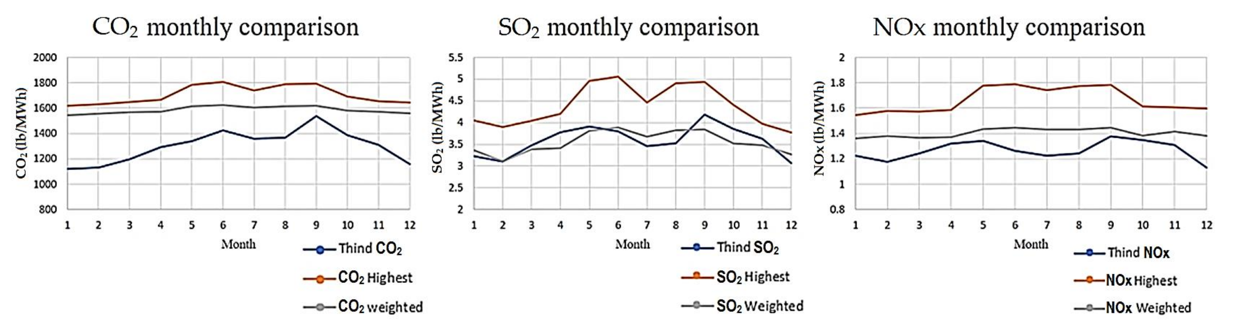
4.2. Monthly MEFs Comparison Results
It is important to consider temporal data in comparing two sets of results generated with different methods that aim to report similar results. As LEEM and Thind et al. both return emission estimations for the same region (MISO), and without a major change in the grid operation over time, the similar emission trends are the most reliable factors to be addressed. Therefore, this study is focused on the similar temporal trends. The emission intensity rates reported by Thind et al. are usually lower than the LEEM intensity rates based on what was observed in the annual comparison.
The monthly comparison demonstration between Thind et al., (2007–2016), and LEEM (2018–2019) in
Figure 3 shows two major emission intensity peaks, one in June and one in September. Although both the weighted and highest probabilities present these peaks, the highest probability shows a more obvious slope. This happens as a result of calculating emissions using the most probable types of fuel and generation technology based on the marginal factors at the margin on a real-time basis. It should be mentioned that LEEM reports the emissions on a five-minute basis rather than hourly (LEEM dataset is of a data resolution that is 12 times more detailed than the Thind et al. dataset), making it fully sensitive to real-time changes in the margin. LEEM does, however, have the same emission trends as the historical data approaches. LEEM estimates emission intensity in two major ways, one is based on the highest probability and the other works based on weighted probability.
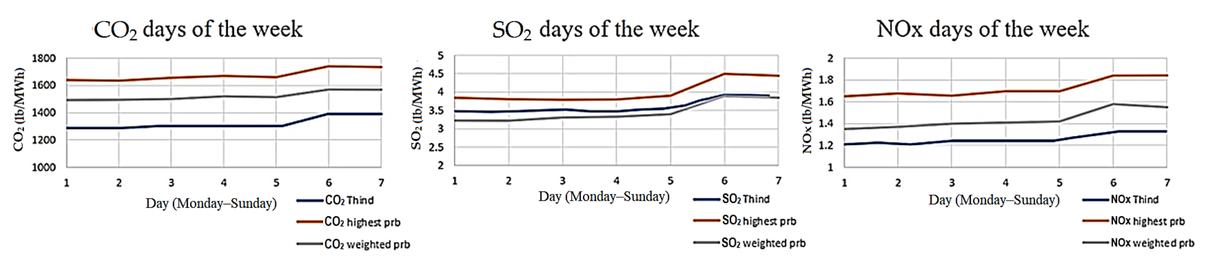
4.3. Daily MEFs Comparison Results
The Thind et al. study analyzed days of the week, showing higher emission intensity at the weekends. LEEM data shows that the fuels used by the electricity generation units are more polluted, and the AMEFs are higher during the weekends (see
Figure 4). The data from LEEM are averaged weeks in the two-years dataset included in this evaluation. However, having higher emission intensity (lb/MWh or kg/MWh) at weekends does not mean that more pollutant is released during the weekends, it only indicates that the fuels on the margin during light load hours on the weekends are coal and natural gas most of the time. Thus, more electricity consumption results in more emissions during the weekends. Moreover, from
Figure 5, which shows the probable share of coal among the total used fuel for an arbitrary LEEM CPN, it can be proved that coal is more on the margin during the weekends than the weekdays.
4.4. Hourly MEFs Comparison Results
The Thind et al. study divided the 24 h of the day into two timeframes, one from 7 p.m. to 7 a.m. and the other from 8 a.m. to 5 p.m. Our study adopted the same policy to make the comparison consistent. As
Figure 6 shows, both LEEM and Thind et al. results show that the AMEFs are higher in the early mornings and late evenings as compared to the other hours. This is due to lower demand at these times, which causes coal to be the main fuel. During the day, the electricity demand is higher, and historically for the Midwest, a wind power plant is the marginal unit. Whenever the emission intensity (lb/MWh) is higher, the used fuel types are more polluted. Coal is used as the base capacity of electricity generation because a coal power plant does not possess a rapid load following capability, whereas natural gas power plants are usually used as flexible and easily adjustable electricity generation units. Averaged LEEM data for 2018 and 2019 represent the same results as the Thind et al. study does.
Table 2 shows that early morning and late evenings (7 p.m. to 7 a.m.) have higher emissions. Thus, the LEEM results are in line with Siler-Evans and Thind et al. results.
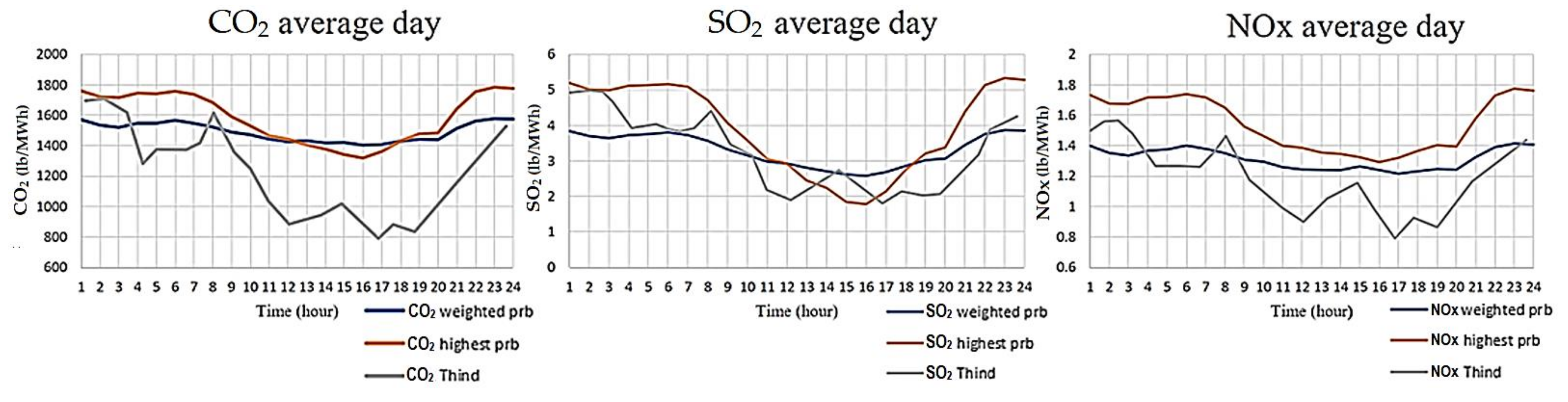
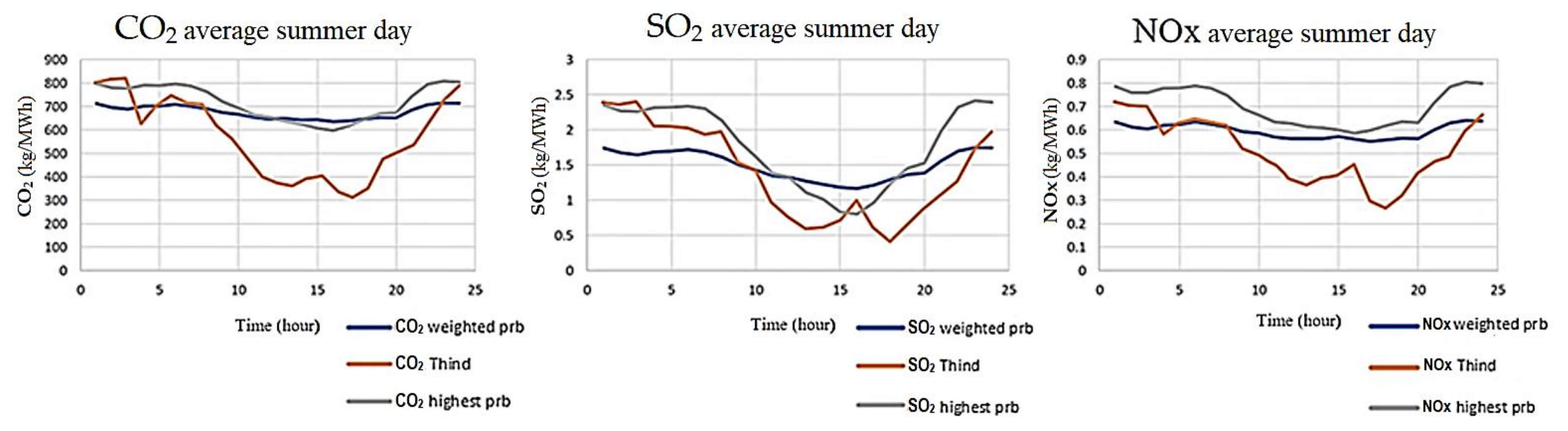
4.5. Seasonal MEFs Comparison Results
The Thind et al. study provided average results in different seasons on an hourly basis. Their results indicated that when there was a temperature change, particularly in winter or summer, there was a spike in the emissions released. LEEM results represented an increase in AMEF amounts when the temperature rose and the demand on the network rose, especially during summer. Below one can see the comparison in 3 different air emissions provided by the Thind et al. and LEEM approaches. For an average day in the summer (see
Figure 7), the highest probability approach shows a better match.
It is notable that Thind et al. [
11] covers the period from 2007 to 2013 (the year MISO changed geographically), whereas LEEM starts from 2018, which explains the differences. Also, Thind et al. presented the data for the whole MISO region, whereas LEEM data is reported for the closest CPN to the WSU campus. The trend of the emission release during 24 h of a summer day shows a reduction in emissions in the middle of the day for both the LEEM approach and that of Thind et al.
As the results show, the emission release is lower during the colder seasons. It may be because cold weather facilitates the cooling process in the cooling towers, which improves the power plant efficiency. Another reason is that during Winter people use gas for space heating, meaning less electricity is consumed. This is unlike the Summers during which electricity is primarily used for space cooling via air conditioning systems, which run on electricity.
Based on what
Figure 7 shows, both the approaches demonstrate peaks in emissions during early morning and late evenings, representing the increase in electricity consumption and absence of renewable energy sources. Lower emissions during mid-day might be because of a more moderate electricity demand and cleaner fuel sources used in power plants. Considering the differences in the approaches, time and geography coverage, the trends show a remarkably satisfying similarity.
5. Discussions and Conclusions
LEEM was developed and tested in the authors’ prior studies, yet no comparison existed that was focused on the different approaches reporting the same type of data. Thus, this study investigated LEEM data reliability by comparing it with two prior studies, including Thind et al., (2017), and CEDM. Thind et al. demonstrated an empirical method based on the data observations sourced from the EPA EIA (CEMS) and the CEDM website, providing the annual AMEFs directly from the same source (CEMS).
The focus of this study is on AMEFs, which are more reliable than AEFs due to the higher sensitivity and precision of AMEFs to the power grid and demand changes. Based on the method developed by Thind et al., (2017), the true environmental benefits of an energy efficiency program will be nearly 20% less than the anticipated outcome when AEFs are used. Also, AEFs overestimate AMEFs by nearly 35% and 25% during the day and night, respectively. The annual AMEFs were made using LEEM data reported for 2018 and 2019, Thind et al., (2017) data from 2007–2016, and CEDM data for 2013, 2017, and 2018 (the most recent year available). The annual comparison showed that LEEM data was closer to the CEDM emission reports by: ~4% closer for CO2, ~12% closer for SO2, and ~11% closer for NOx. There is a limitation in the Thind et al. approach, where this empirical approach calculates MEFs on fossil fuel power plants larger than 25 MW. LEEM does not have any limitations in the type of fuel or power plant. Other temporal comparisons, including the seasonal, monthly, days of the week, and hours of the day, result in similar trends. It is satisfying to see that a stochastic approach returns the same patterns that a historical approach does. However, the temporal AMEFs for Thind et al. were generally lower than the LEEM AMEFs, which are justifiable because the annual averages for Thind et al. are lower in all emission estimations.
Monthly investigations present two peak months during the year for emissions released for both datasets. Days of the week comparison showed that the emission intensities during the weekends are higher than during the weekdays in both LEEM and the Thind et al study. The hourly investigation demonstrates higher emission intensity during early morning and late evening in both LEEM and Thind et al. Seasonally, in summer, average hourly emission comparison projects the same patterns for both the LEEM dataset and the Thind et al. dataset, showing two emission peaks in the same months.
LEEM provides more detailed and informative reports compared to prior studies. In LEEM, the data resolution of the reports is five-minutes, which is much more precise than that of the prior approaches. As a unique feature of LEEM, it can be said that the data is calculated in a real-time format with no limitation in the type of power plant and fuel sources for any specific location, which demonstrated the geographical sensitivity of LEEM. For instance, data is calculated on a real-time basis for every transmission bus in Michigan (182 locations).
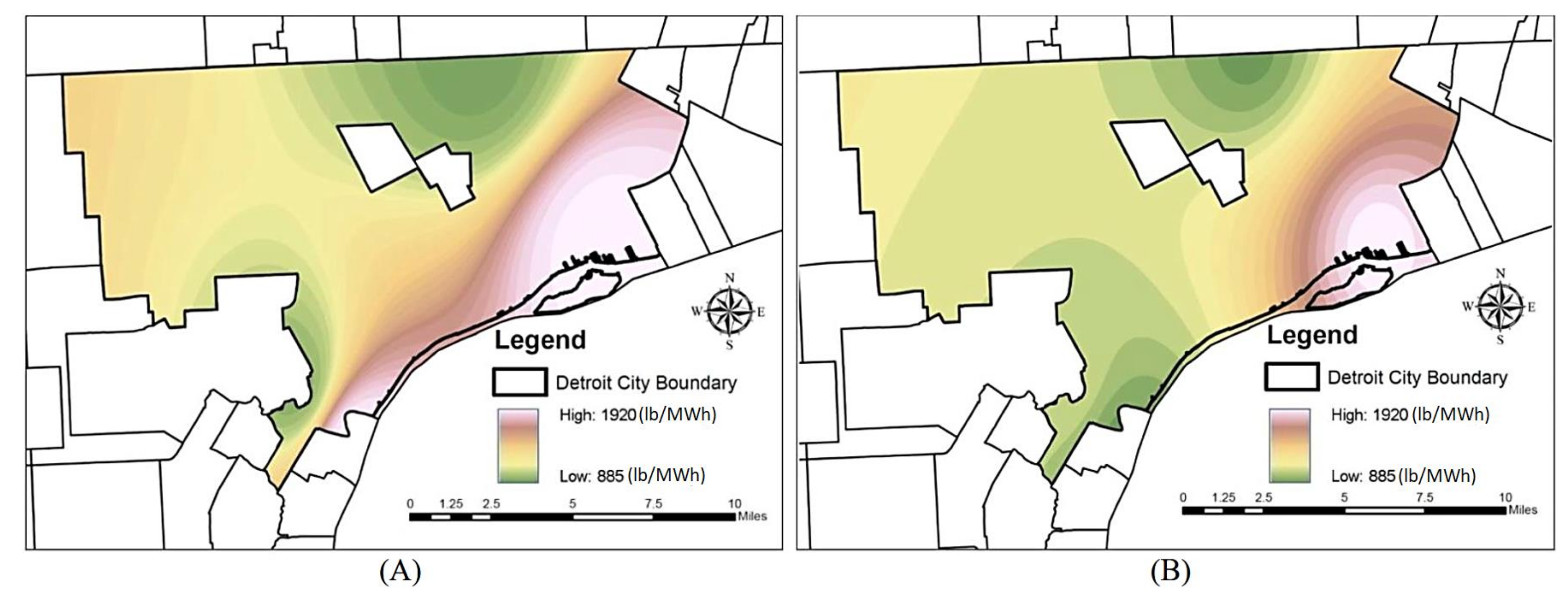
Figure 8 shows a map of LEEM data generated for a random date using different CPN emission intensities for Detroit City. The figure shows the CO
2 emissions for both the light load and heavy load hours. Regional temperature change directly affects the LMPs. The power demand on the transmission system changes as the consumers start to use more electricity for air conditioning purposes. The operators of power systems call on power plants to produce and place the right amount of electricity supply on the grid at every moment to instantaneously keep the supply and demand balanced. The historical approaches are unable to address the emission estimation rise as they are not using an approach that is sufficiently sensitive to the changes on the margin.
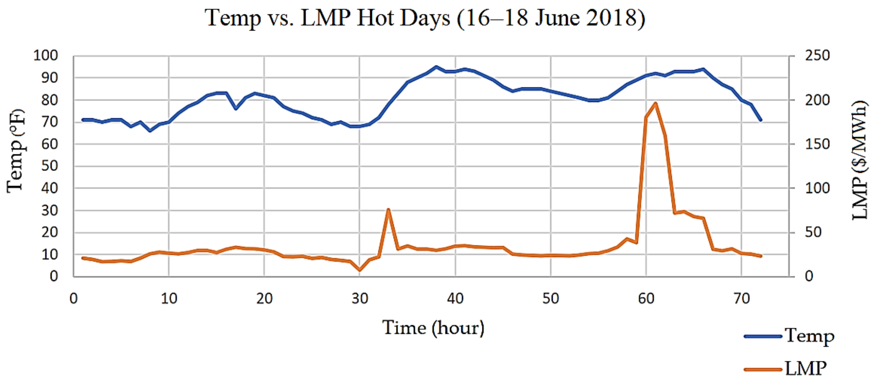
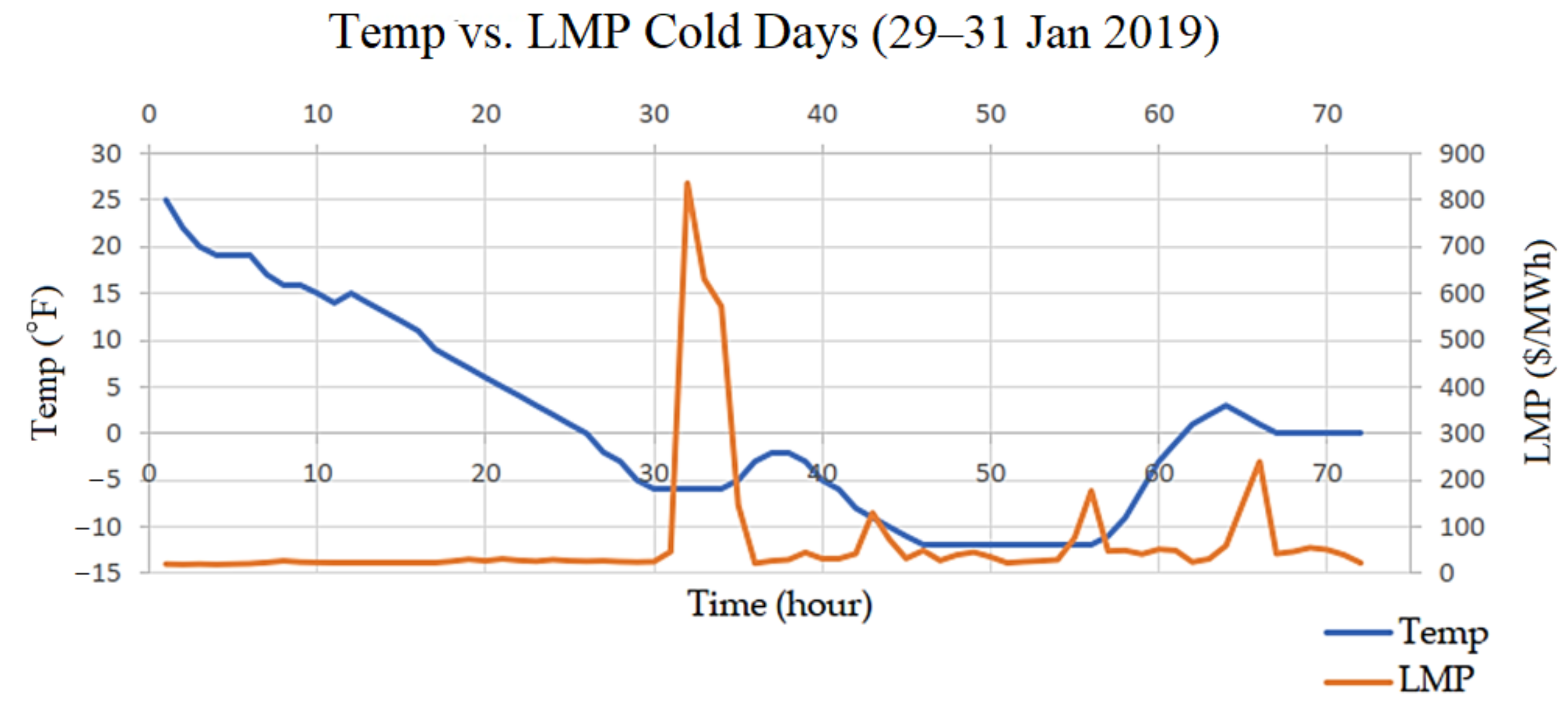
Figure 9 and
Figure 10 demonstrate how hot/cold weather affects the LMPs. Since LEEM is a real-time LMP based stochastic approach, which is geographically sensitive to the marginal factors on the grid, it is able to fully address the emissions.
Potentially, LEEM can deliver emission intensity real-time information to residential sectors as well as utilities and industries. Due to the locational feature of LEEM, which gives data per location, LEEM can be used to provide accurate and real-time information to residential consumers. In 2018, retail sales of electricity to 3 major end-use sectors were 1464 billion kWh for residential, 1377 billion kWh for commercial, and 953 billion kWh for the industrial section [
34]. Other than impacting energy efficiency and shifting the electricity usage from peak hours to light load hours, there is a great potential to motivate individuals to change their electricity usage behavior according to the environmental and economic information. Public awareness is of a key role in altering the behavior of individuals towards a significant improvement in energy usage regimen; therefore, it is obligatory to enhance public awareness about the benefits that energy consumers will receive in exchange for their behavior change. Some recent studies [
35,
36], which investigated the customers’ willingness to adopt renewable energy in highly populated countries like China and Pakistan, has also supported the importance of enhancing self-effectiveness and public awareness. In regard to the untapped potential of energy saving and emission reduction in the US residential sector, it is beneficial to deliver emission information to the residents and give them the chance to not only save money and energy but also to reduce the emissions caused due to electricity generation.


