Reducing Global Greenhouse Gas Emissions to Meet Climate Targets—A Comprehensive Quantification and Reasonable Options

Kern, Christoph; Jess, Andreas

doi:10.3390/en14175260

Open AccessArticle

Reducing Global Greenhouse Gas Emissions to Meet Climate Targets—A Comprehensive Quantification and Reasonable Options

by

Christoph Kern

and

Andreas Jess

^*

Chair of Chemical Engineering, Center of Energy Technology, University Bayreuth, 95440 Bayreuth, Germany

^*

Author to whom correspondence should be addressed.

Energies 2021, 14(17), 5260; https://doi.org/10.3390/en14175260

Submission received: 28 July 2021 / Revised: 19 August 2021 / Accepted: 20 August 2021 / Published: 25 August 2021

(This article belongs to the Section B: Energy and Environment)

Download

Browse Figures

Versions Notes

Abstract

:

A model is presented which covers the global greenhouse gas emissions (GHG emissions) and the energy consumption (fuels, electricity) in five sectors of end users, industry, transport, buildings, agriculture, and fugitive emissions. The electricity sector is also considered, but the associated GHG emissions are reallocated to the five end users. Different GHG reduction measures were calculated ranging from substitution of coal for electricity generation by renewables, electrification of road transport and buildings, restructuring of the sector industry to finally a 50% reduction of both food waste and meat consumption. To elucidate the consequences of global warming, future emission scenarios were also incorporated. One major conclusion is that the world can only reach the 2-degree climate target if electricity is only produced by renewables, and if transportation, buildings, and the industry are completely electrified by 2050. Compared to today, the electricity production by renewables will then rise by a factor of 11, and the total electricity demand by a factor of 2.4.

Keywords:

energy transition; greenhouse gas emissions; climate policies

1. Introduction

Publications on greenhouse gas emissions (GHG emissions), climate change, and climate targets and policies are numerous, ranging from scientific publications, popular scientific books, such as the recently released book written by Bill Gates [1], and newspaper articles to statements as well as pledges of governments and political parties.

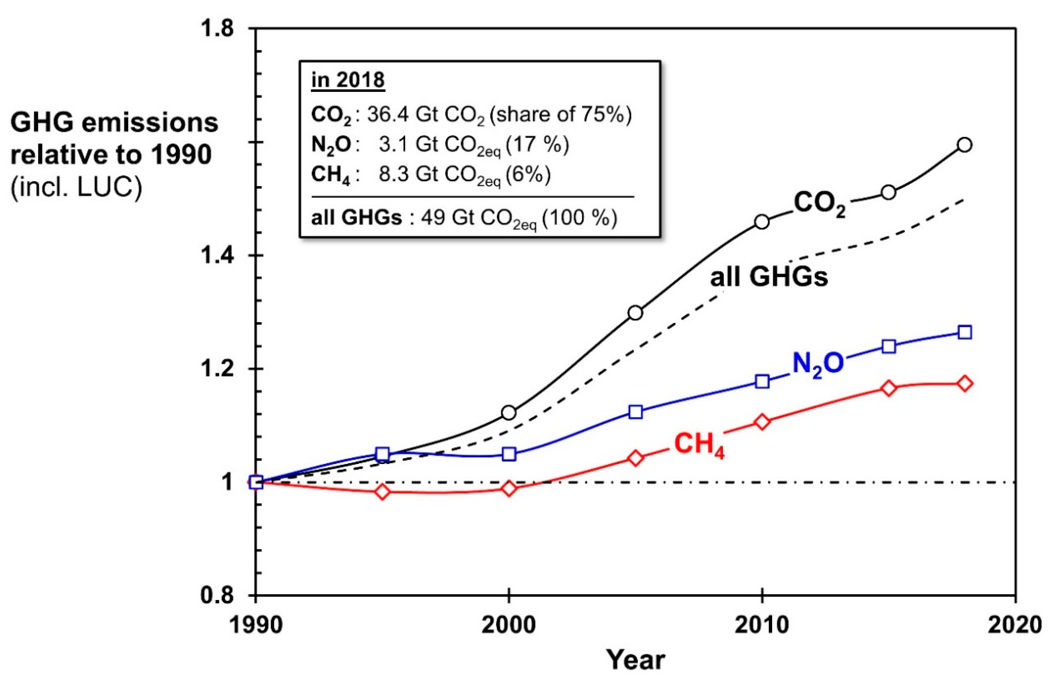
Without any doubt, greenhouse gas emissions have strongly increased during the last decades, as shown in Figure 1. Herein, the emissions of the most relevant greenhouse gases, i.e., carbon dioxide, nitrous oxide, and methane, are given for the period of 1990 to 2018. According to the data shown, the emissions of CO₂ have increased by 60%, the output of methane has grown by 17% and the emissions of N₂O have risen by 26%. These three gases have currently a share of 98% on the total greenhouse gas emissions, CO₂ has a share of 75% whereas methane and N₂O participate with a share of 17% and 6%, respectively. The emissions of fluorinated GHGs (F-gases; not depicted in Figure 1) have significantly gone up by a factor of 4, but the share of 2% is still small. In total, the overall greenhouse gas emissions today are about 50% higher than in 1990.

Although the general trend of GHG emissions is rising, there are massive differences between countries and regions responsible for the greenhouse gas emissions (Table 1). Industrialized countries in North America and Europe have reduced their total and per capita GHG emissions in the last three decades by up to about 25%. However, both the per capita and the total emissions of emerging nations like China and India have increased quite strongly. In some African countries such as Nigeria, per capita emissions have decreased, but the total emissions have gone up because of the strong growth of the country’s population during the last decades.

Interestingly, the per capita emissions have almost remained constant from 1990 until today globally (Table 1). In other words, on global average, the rise in GHG emissions is mainly the result of the growth of the world’s population from 5.3 billion in 1990 to 7.9 billion today (July 2021). Table 1 also lists the greenhouse gas emissions relative to gross domestic product (GDP) and the human development index in the named countries. One issue should be noted here: China’s emissions of greenhouse gases per 1000 US $ GDP are remarkably high with 0.6 t CO_2eq (global average 0.4 t CO_2eq). This is the result of China’s tremendous coal demand: 50% of the global coal is consumed only by China and coal is still the dominating primary energy source of China with a share of 62% compared to 27% on global average in 2019.

As already mentioned, there are numerous publications on GHG emissions and on scenarios of their reduction, but they mainly concentrate on emission pathways to reach a certain climate target, e.g., to limit the global temperature rise to a defined value such as 1.5 °C or 2 °C, relative to pre-industrial temperatures. Hence, emissions reduction targets and the point in time of achievement such as 50% reduction in 2050 are of top priority. Other investigations concentrate on ways and means to reduce emissions in certain sectors such as electricity generation, transportation, buildings, industrial processes, or agriculture. All these issues are undoubtful important, but the strong link of all sectors of end users is seldom considered. However, this is an absolute must to evaluate the outcome of different actions and measures on GHG emissions and climate change. Hence, a realistic and feasible course of action from an engineering orientated perspective is mostly not presented or remains rather vague.

Even the allocation of GHG emissions to certain sectors is not an easy task, as shown in Table 2 by comparison of data published by Gates in his new (worth reading) book [1] and our calculations (based on published data) presented in the subsequent chapters.

Gates claims that the industry is the major GHG emitter, responsible for 31%, and electricity is only second (27%). This is not the case or at least a problem of double counting: If electricity is counted as an own sector, as Gates obviously did, GHG emissions of end users such as industry, buildings and transportation must be given without their electricity consumption, or the electricity produced has to be (re)allocated to all end users. This is probably more appropriate, e.g., to show what the share of end users actually is. In any case, a proper allocation of GHG emissions to sectors is needed. Sectors of end users—whether they include electricity demand or not—are strongly interlinked, which must be considered when judging GHG reduction measures. For example, reducing the consumption of oil products for transport will also decrease the emissions of oil refineries and fugitive emissions related to oil production, currently responsible for 4% of global GHG emissions; even more significant is the substitution of coal for electricity by renewables, as this will lead to less emissions by end users such as industry or transport if e.g., cars with currently internal combustion engines (ICE) are substituted by electric vehicles.

In this paper, a reliable tool and model is presented, which is comprehensible and comprehensive, as it covers the GHG emissions and the consumption of electricity as well as the demand of fossil and other fuels in all interlinked sectors of end users on a global basis. An issue of particular importance—and our main motivation to develop such a tool—is the opportunity of the model to run freely through simulations and future scenarios, of course within the constraints of today’s technical capabilities. Hence, this paper concentrates on the current technical options to reduce GHG emissions, on the respective consequences both regarding the degree of reduction of GHG emissions and the excess consumption of electricity

In the upcoming Section, the basis or our global model is presented. In Section 3, calculated data for the base case of the year 2016 are compared with literature data to confirm the model. In Section 4, GHG reduction pathways, as calculated by the model, are outlined. Finally, in Section 5, energy transition pathways and global warming scenarios are discussed. Not being experts in climate research, we focus on technical options to reduce GHG emissions and use published trajectories to estimate the impact on global warming and the achievement of climate targets.

2. Methodology

In the model developed for this paper, the global energy system was divided into five sectors of end users and the sector electricity & heat. The outcome of the latter, generated electricity and GHG emissions, was reallocated to the end users according to their electricity demand (Figure 2).

Table 3 and Table 4 exemplarily show the respective data for the sectors transport and electricity and heat, respectively. The sector transport considers the consumption of fuels and of the small amount of electricity currently consumed herein. All transportation modes (Table 3) were considered, i.e., road (mainly gasoline and diesel oil), rail (diesel, electricity), air (jet-fuel), ship (gasoil/diesel oil), and pipeline (electricity). The sector electricity & heat (Table 4; 84% electricity, 16% heat) accounts for all power and heat plants run by fossil fuels, biomass, nuclear, hydro, solar, wind, or geothermal energy. The fuel in- and the output of electricity/heat are calculated. Own use of electricity and losses during transport of electricity are also incorporated. The Table 3 and Table 4 (and the Tables S2–S4, S9 and S10 in the Supplementary Information) are divided in sections with different background colors: Red indicates data valid for today, and green data if the reduction of GHG emissions is maximized by the measures considered here; the blue color in Table S4 and grey and yellow in Table 3 are special cases explained in the table.

Data of the other sectors can be found in the Supplementary Information. The sector industry consists of subsectors, iron & steel (Table S2), cement (Table S3), chemical and petrochemical industry (Table S4), non-ferrous metals (Table S5), industrial processes related to machinery, food, tobacco, paper, pulp and printing (Table S6), and other processes (Table S7). The data were taken from literature [2,5,6,7,8,9,10,11,12,13,14,15,16,17,18,19,20,21]; for details see Table 3 and Table 4, and Tables S1–S7. The own use of electricity and fuels of power & heat plants and refineries and losses of electricity during transport (Table S8) were attributed to industry, although electricity is also used to about the same extent for buildings (Table S9). However, such allocations have no influence on the global reduction of GHG emissions and are appropriate to reach a manageable number of sectors, here five. The sector residential & commercial buildings considers the consumption of fossil fuels (coal, heating oil, natural gas), modern/traditional biomass, electricity, and district heat (Table S9). CH₄ and N₂O emissions of burning of traditional biomass are also assigned to this sector.

The sector agriculture (Table S10) incorporates emissions of CO₂, CH₄, and N₂O from burning of agricultural residues, CH₄ from livestock, manure and rice cultivation, N₂O from agricultural soils, and emission related to consumption of fossil fuels, biofuels, and electricity. Emissions from LUC (deforestation, cropland) and CH₄ from landfills and wastewater were also attributed. The worldwide ongoing forest and vegetation fires (e.g., California, Turkey, Greece), exceptionally strong in 2021, represent both a major effect and a cause of the global GHG emissions. This may lead in future to an increasing contribution of this sector to the global GHG emissions, but this aspect is far beyond the scope of this work and was not considered in the model.

In the last and smallest end user sector (other), some remaining emissions not easy to allocate to other end users are merged: N₂O and CH₄ from burning of fossil fuels and fugitive emissions of CH₄ and CO₂ related to leakages, flaring, and coal mining (details in Table S1).

In each sector of end users, consumption of fuels and electricity is specified in metric tons of oil equivalent (41.9 GJ/toe). The CO₂ emissions are calculated by applying emission factors, compiled on the basis of average carbon content of the (fossil) fuel, 3.96 t CO₂ per toe coal, and 2.35 and 3.07 t CO₂ per toe of natural gas and oil (products), respectively [7]. The respective emission factor for electrical energy depends on the fuel mix of electricity generation and is calculated in sector electricity & heat.

The GHG emissions data of all sectors, including the emissions of CH₄, N₂O, and F-gases, were mainly collected from the numbers published by the World Resources Institute (WRI) [2]. For 2016, the WRI provides the latest update of global GHG emissions in detail, i.e., sectors, gases, end users. Thus, 2016 was therefore used here as base case. In most cases, electricity and fuel consumption could be recalculated by (reciprocal) emission factors, e.g., for road transport by the factor 0.326 toe crude oil product per t CO₂ emitted (=reciprocal value of 3.07 t CO₂ per toe oil). In some cases, complementary information from literature was used to specify the consumption of electricity, oil, gas, or coal in each sector, e.g., in the subsectors of the sector industry. This was also helpful to prove the plausibility of numbers (details in Table 3 and Table 4, and Tables S1–S13 in the Supplementary Information).

The numbers of GHG emissions given by the WRI [2] for production of electricity and of heat by combined heat and power plants (CHP) or heat plants are not specified with regard to the amount and shares of fossil fuels, nuclear and renewable energy. Hence, data of consumption of natural gas, crude oil (products), coal, and biomass in power plants as well as of renewable electricity (wind, solar, hydro) and nuclear power published by the International Energy Agency (IEA) [8] were utilized (Table 4). The global emissions of CO₂ related to electricity & heat generation calculated on the basis of the IEA numbers (14.7 Gt CO₂) correspond well to the number given by the WRI (15.0 Gt CO₂). The generated electricity, 2.66 Gtoe including own use of power plants and transport losses, was calculated based on the electricity demand of all five end user sectors. It also agrees well with the number published by the IEA [8] for 2016 (2.73 Gtoe). The average emission factor per unit electricity/heat, a major outcome of model sector electricity, is 5.14 t CO₂ per toe of electricity in the base case of the year 2016.

The results of the calculations—GHG emissions and consumption of fuels and electricity for 2016—will be discussed in more detail in chapter 3. However, much more important and the main reason for developing the model has been the option to calculate future scenarios of GHG reductions options (chapters 4 and 5). The data were therefore implemented in Microsoft Excel 2019 (running on a workstation with an Intel i7-8700 CPU @ 3.20GHz) with the following additional tools on the basis of literature data where needed (see Table 3 and Table 4, Tables S4, S9 and S10, particularly sections with green background color): For each subsector within industry, today in total responsible for 36% of the GHG emissions (including the allocated electricity demand), the consumption of fossil fuels can be changed (normally reduced to decrease GHG emissions), whereby the appropriate change (increase) of the electricity demand is considered (1 toe fuel = 1 toe electrical energy). Tables S2–S4 depict this procedure for iron & steel, cement, and the chemical/petrochemical industry for the maximum reduction of greenhouse gas emissions. For iron & steel, coal/coke (blast furnace) can be completely replaced by (renewable) hydrogen as reducing agent (Table S2). For cement, process heat can be delivered (in the model) by electrical energy, but the CO₂ emissions related to by-product formation resulting from calcination of limestone must be accepted. Hence, CO₂ separation and sequestration or use, which may be future options, were here disregarded, but may be of interest for further model calculations, and can be implemented into the model.

The share of fuels and electricity in the sector transportation, currently responsible for 17% of total global GHG emissions, can be varied in the model, whereby it was assumed (until now) that aviation and shipping are still based on crude oil products. For road transport, cars with internal combustion engines (ICEs) can be replaced partly or completely by battery electric vehicles (BEVs) and trucks with ICE by hydrogen fuel cell vehicles (HFCVs). The additional electricity demand (increase) connected to these changes is calculated by tank-to-wheel efficiencies and the current efficiency of H₂ production by electrolysis (70%); for details see [9] and Table S11.

A similar switch from coal, heating oil, and gas to electricity is considered in sector buildings with a current share of 18% of global GHG emissions, assuming that (electrical) heat pumps are used instead of fossil fuels. The substitution factor is 0.33 toe electrical energy per toe oil or gas, see best case in Table S9.

In the sector agriculture, currently responsible for 22% of GHG emissions, fossil fuels can be substituted by electricity, although the effect is rather small, as the share of fossil fuels within the greenhouse gas emissions in agriculture is only 7% (Table S10). Much more effective with regard to reduce GHG emissions is the reduction of the amount of waste/losses of food, currently 24%, and meat consumption. Hence, both aspects were implemented into the model (see Table S12). In Section 4, the results for 50% reduction of both food waste and meat consumption are presented as an instructive example.

In the smallest sector other with a share of 7% on total GHG emissions in 2016, emissions of N₂O and CH₄ from burning of fossil fuels and fugitive emissions of leakages, flaring, and coal mining are calculated. Thus, if the consumption of a fossil fuel decreases relative to the base case, e.g., coal is replaced by wind energy in the sector electricity or less crude oil products are consumed in transport (BEV and HFCV instead of ICE for cars and trucks, respectively), the GHG emissions of this sector declines.

In sector electricity & heat (Table 4), the shares of primary energy sources can be altered. In the scenarios considered here, wind or solar power substitutes fossil fuels. The amount of electricity produced by modern biomass and nuclear power were “frozen” to the values of 2016, 0.09 Gtoe and 0.23 Gtoe electricity, respectively. Thus, it was assumed that the existing biomass-based and nuclear power plants will be still in operation in the near future.

Finally, the model provides sensible numbers of the non-energetic use of fossil fuels, mainly natural gas and coal as feedstock for ammonia and methanol; and crude oil for bitumen, lubricants, olefins and aromatics (see Table S13). This has no influence on the GHG emissions but was implemented in the model to determine the global consumption of each fossil fuel in different scenarios. Note that CO2 formation as by-product of ammonia production is already considered in the subsector chemical & petrochemical industry (Table S4).

3. Global Data of GHG Emissions and Energy Consumption for the Base Case 2016: Comparison of Model and Literature Data

Table 5 depicts a comparison of data calculated by the model for the year 2016 with data from literature. As already mentioned before, the model matches “real” data of fossil fuel consumption, electricity generation, and GHG emissions very well. This is partly not astonishing, as literature data are the basis of the model. But it shows at least that the energy consumption data of the IEA and GHG emission data of the WRI are reasonable and that both data sets fit nicely together; and this also underlines the suitability of the model.

Table 6 shows the global emissions of all four relevant GHGs allocated to five end user sectors. It is remarkable that the sector agriculture is (behind industry) the second largest emitter of GHG, whereby CH₄ and N₂O dominate this sector with a share of about 70%. CO₂ is mainly emitted by the sector industry (45%) followed by buildings (23%) and transportation (22%). It should be noted that the F-gases are completely allocated to sector industry via subsector chemicals and petrochemical industry, although the real emissions of F-gases appear during the use and disposal of refrigerators, air conditioners, or fire-extinguishers.

4. GHG Reduction and Energy Transition Pathways

Table 7 gives an overview of the measures M_i considered in this work to reduce GHG emissions (with i = 0 for base case and 1 to 6 for successive actions). Both the global population and the average prosperity (heat demand, use of different modes of transportation, industrial production of materials and goods) are here, to begin with, considered as constant.

It must be emphasized that future measures to reduce greenhouse gas emissions will not be taken one by one, but parallel or at least overlapping. However, we have still used the succession of different measures, as this clearly illustrates the individual influence of each measure on the reduction of GHG emissions; their chronological order was chosen on the basis of the most effective measure that is (still) available at a time, i.e., the action with the lowest additional electricity demand per t CO₂ saved. In addition, if, for example, two measures are implemented bit by bit in parallel—as it will be certainly the case -, the final value of the GHG emissions reached will be the same. The only difference is or might be the value of the cumulative greenhouse gases emissions released during a certain period in time. However, this effect, disregarded in this paper, is rather small: For example, if the measures 1 and 2 (see Table 7) are implemented to only 50% each in a certain period (e.g., 10 years), and in the following period of equal length then completely, this would only increase the cumulative GHG emissions by 1% compared to the approach in this work, i.e., measure M₁ completed in period 1 and M₂ in the subsequent period.

Figure 3, Figure 4 and Figure 5 depict the shares of CO₂, CH₄, N₂O, and F-gases (Figure 3), those of different end users (Figure 4), and the reduction of emissions of CO₂, CH₄, N₂O (Figure 5). The shares of nuclear power, renewables and fossil fuels within electricity generation are shown in Figure 6. The consumption of fossil fuels in 2016 as well as if consecutive measures are taken are given in Figure 7. Additional data can be found in Tables S14 and S15.

The Figure 3, Figure 4, Figure 5, Figure 6 and Figure 7 are largely self-explanatory, and only main conclusions should be highlighted: The by far best initial measure to reduce GHG emissions is substitution of coal in sector electricity by renewables, as this would reduce global emissions by 21%. The emission factor strongly drops from 5.1 (2016) to 1.5 t CO₂ per toe electricity, which is a prerequisite of the success of subsequent measures. For example, electrification of transportation (M₂) would reduce the global GHG emissions by 3% (and by 14% in sector transport) for the current electricity mix (Table 3, yellow background) compared to 36% reduction if combined with M₁ (coal substitution in sector electricity).

If the additional electricity needed for transportation would be generated by coal-fired power plants, of course counterproductive for reduction of GHG emissions and only mentioned for comparison, the GHG emissions would be even 46% higher than before (Table 3, grey background).

The current global capacity of coal power is about 2000 GW ([22], Table S16) and has increased on average by 3% per year in the period 2009 to 2019, but in China and India by even 6% and 10%, and in other parts of Asia by 5%. Only in the European Union and in the US, the capacity of coal power is shrinking, in both cases by 3% per year in the last decade. It is unlikely that Asian coal power plants with a share of 70% of global coal power will be speedy shut down. Substitution of coal is challenging in China and India with shares of coal in primary energy of 62% and 45%, compared to the US or the EU28 with both only 14% in 2019 (Table S16).

Additional issues are the low-capacity factors (CF), i.e., the average actual electricity output divided by the rated maximum possible peak value, of wind and PV power due to their fluctuating nature, 10% to 25% compared to 70% for coal. Hence, the current 2000 GW of coal power must be substituted by at least 7000 GW wind power or PV (for CF = 0.2). This is not at all an easy task, as today´s globally installed capacities are only 700 GW for wind and 600 GW for PV (2019 [23]). Huge wind turbines have a capacity between 5 MW (on-shore) and 10 MW (off-shore). Hence, about one million new turbines would be needed.

If the sector building is also electrified by measure 3, i.e., heat pumps substitute heating by oil and gas, the reduction of GHG emissions would reach 44%. The two most important remaining sectors are then agriculture and industry with shares on GHG emissions of 36% and 42%, respectively (Figure 4). If electricity is completely generated by renewables (or nuclear power) by measure 4, shut down of gas- and oil-fired power plants, we reach 54% GHG emissions reduction. The remaining 46% are mainly attributed to the sectors industry and agriculture (incl. LUC).

By measure 5, a strong restructuring of the sector industry is presumed. The main drivers are the subsectors iron & steel, cement, and chemical and petrochemical industry, today with a share of 70% of all industrial GHG emissions (Table S17). Currently, 1.8 Gt CO₂ are related to coke for iron & steel, 3 Gt CO₂ to cement (coal as fuel, byproduct), and 1.1 Gt CO₂ to byproducts of petrochemicals. This is in total 5.9 Gt CO₂, 12% of current global total GHG emissions, which are hard to avoid by today´s technologies. Nevertheless, measure 5 assumes an almost completely electrified industry. Steel is only produced with renewable hydrogen as the reduction agent, and production of F-gases (1 Gt CO_2eq) is abandoned. The remaining industrial GHG emissions are unavoidable CO₂ emissions of limestone calcination (1.5 Gt CO₂) and minor N₂O and CO₂ emissions related to ammonia production on the basis of natural gas and of nitric acid (each 0.2 Gt CO_2eq).

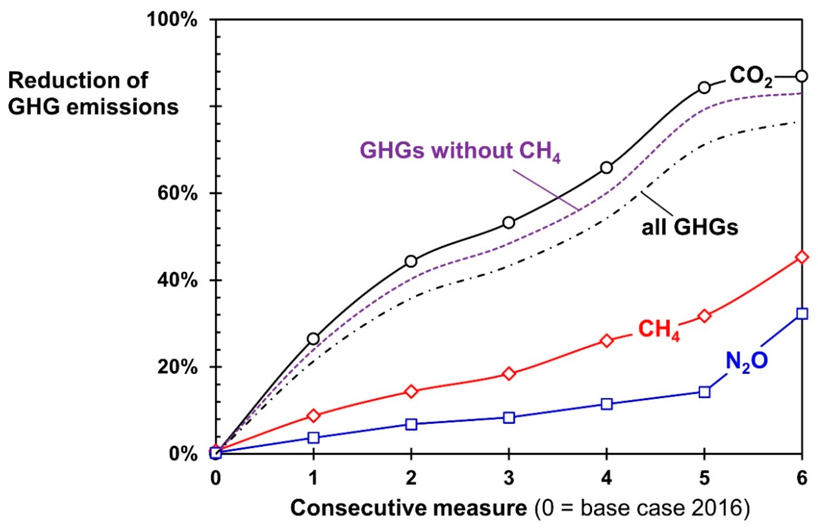
If all five measures are taken, a reduction of the GHG emissions by 71% is achieved. Agriculture is then the by far dominating remaining emitter with a share of 68%, mainly methane with a fraction of 55% and nitrous oxide with 25% within GHG emissions of agriculture, followed by industry (15%) and transport (12%), Figure 4. As a result, the total CH₄ emissions decline to a lower extent compared to CO₂, 30% vs. 80% (Figure 5), and the share of methane on the overall GHG emissions rises with increasing reduction of total GHG emissions (Figure 3), from 17% to 40% if the measures 1 to 5 are taken.

Without going into details: The at first glance small reduction of the methane emissions by 30%, as projected here for the measures 1 to 5, would be favourable regarding climate change, as the atmospheric residence time of methane is only 12 years. According to a recently published study on the global methane budget [24], the atmospheric methane content would decrease from today´s value of 1800 ppb to around 1400 ppb in 2050 if the global methane emissions would be continuously reduced to 70% of today´s value until 2050. (For nitrous oxide we have a mean residence time of 120 years; the lifetime of CO₂ is hard to determine, because there are several processes removing CO₂ from the atmosphere. Most likely about 1/3 of the anthropogenic CO₂ emissions are still present in the atmosphere even after 100 years.)

Consumption of fossil fuels is reduced by 87% and only used for fuels for shipping and aviation (Figure 7) and for the petrochemical industry as feedstock (Table S4). It is by no means a herculean task to reach this goal, above all on global average and in only a few decades.

The last measure (no. 6) considered in this work is the effect of 50% reduction of food waste and of 50% less meat consumption. (It is far beyond the objective of this paper to discuss the pros and cons of vegetarian nutrition and the cultural consequences of agriculture with much less or even no animals.) Within the food supply chain, 24% of the food (related to kcal) is lost or wasted [25]. 5.3 Gt CO_2eq, around 50% of total food and 10% of GHG emissions in 2016, are related to meat production (incl. fish/seafood), 1.9 to milk and eggs, and 3.9 to non-animal food, in total 11.1 Gt CO_2eq [26]. A decrease of 50% of GHG emissions attributed to animals is unrealistic, as additional crops and more synthetic fertilizers are then needed. Greenhouse gas emissions of non-animal food will increase by 40% and the total emissions without meat will be 7.3 Gt CO_2eq (=1.86 + 1.4 × 3.9), which corresponds to a reduction of 34% compared to today. This value was used in the model presented here. A similar value is also given by White and Hall [27]. They calculated (for a complete removal of animals from agriculture in the US) a reduction of 30% because of the production of additional crops on land previously used by animals (32% increase over plant contributions in the system with animals), the need to synthesize fertilizers to replace animal manures (7% increase), and disposal of human-inedible byproducts as feed for animals (+1%). All in all, 50% less meat + 50% less food waste would increase the reduction of GHG emissions from 71% (measures 1 to 5) to 77%. Hence, less meat and food waste would have an effect, although smaller compared to the other measures discussed here. For example, a substitution of coal for electricity by renewables by 30% would have the same effect as 50% less food waste and 50% less meat. For 50% less meat at constant waste a reduction of coal for electricity by 20% would be “sufficient”.

One important point that always must be taken into account for all GHG reduction strategies is that in any case electricity production in total and based on renewables (or alternatively by nuclear power, which is here not considered) will increase quite dramatically (Figure 8). For example, a reduction of GHG emissions by 54% (by measures 1 to 4) would increase the global annual electricity demand from today 2.7 Gtoe to 4.2 Gtoe (+56%). Currently (2016), only 0.6 Gtoe electricity is based on renewables, hence 3.4 Gtoe more renewable electricity—probably mainly by wind and PV—would be needed (assuming nuclear power still delivers 0.2 Gtoe as today). A further rise of total annual electricity demand from 4.2 to even 6.2 Gtoe, i.e., an increase of renewable electricity compared to today (0.6 Gtoe) by a factor of 11 would then be needed if the sector industry is also electrified (measure 5). Compared to the total electricity demand of today (2.7 Gtoe), 6.4 Gtoe (factor 2.4 more) electricity is then needed.

Figure 8 indicates that the effort needed to save GHG emissions, for example expressed as additional electricity demand in toe per t CO₂ saved, will increase with the degree of overall reduction of GHG emissions. For substitution of coal by renewables in electricity, we have 0.09 toe electricity per t CO₂, for electrification of transport and buildings 0.14 toe/t CO₂, and finally for the restructuring of the industry a high value of 0.26 toe per t CO₂ (details in Table S14). This underlines that the proposed sequence of measures, although in “real” life done partly in parallel, is conducive.

Until now, the question how fast the different measures should be implemented, was not addressed. In the following and final section, the outcome of the model will therefore now be compared with different global warming scenarios.

It should be finally mentioned that the global primary energy (PE) demand is not altered by the measures 1 to 4, and only slightly increases by measure 5 if electrical energy (EE) generated by renewables is still—as today in a world mainly run on the basis of fossil fuels—converted in PE by assuming an efficiency of 40%, i.e., 1 Gtoe EE equals 2.5 Gtoe PE. In a predominant renewable world, EE to PE conversion is senseless, and the global energy then decreases if we go from the base case (2016) to consecutive measures, see Figure S1.

5. Energy Transition Pathways and Global Warming Scenarios

What does the future of the global greenhouse gas emissions look like? Figure 9 shows a range of potential future scenarios of global GHG emissions based on data of Climate Action Tracker [28]. Here, the following four scenarios are shown:

○: Current climate policies will lead to a projected warming by 2.7 to 3.1 °C by 2100.
○: Pledges and targets: All countries achieve their current targets/pledges set within the Paris climate agreement with an average warming by 2100 of about 2.4 °C.
○: 2 °C pathways: There are several emission pathways compatible with limiting average warming to 2 °C by 2100, but this would require a significant increase of current pledges.
○: 1.5 °C pathways: very urgent and rapid reduction in global GHG emissions.

All these scenarios have a certain confidence interval of value due to the uncertainty of scenario studies as indicated in Figure 9.

To elucidate the future of GHG emissions and their consequences on global warming, we have assumed here that the six consecutive measures described above to reduce the GHG emissions are available and can be applied. The effect of the projected increase of global population from 7.8 billion in 2020 to 10 billion in 2050—and thereafter assumed to stay constant—was also now considered simply by assuming a linear relationship of population and GHG emissions. For example, a reduction of GHG emissions by 21% by measure 1 (shut down of coal power plants) if taken today, decreases only to 16% if realized after 2050 (21% × 7.8/10). This assumption of a linear relationship of population and GHG emissions is debatable since population growth occurs mainly in low-income countries with lower GHG emissions per capita in the next decades. This may lead, if not “(over)compensated” by emerging economies, to a lower GHG emissions pc in 2050 than in 2016 so that the calculated trajectory (blue data points) shown in Figure 9 is overestimated. Nevertheless, we think that the assumption is reasonable, as otherwise the growth of the world population is ignored. Other aspects such as potential changes of global average prosperity, expected for emerging economies, were simplifying disregarded.

Figure 9 also shows the trajectory of the annual GHG emissions (M₁ to M₆) in the next decades that exactly follows the 2 K pathway. (The corresponding changes of the renewable electricity demand of this pathway and the years, when each measure should be finalized are shown in Figure S2.)

There is one major conclusion can be drawn from Figure 9: It will be very hard to reach the target of 2 °C warming compared to pre-industrial time (and the 1.5 °C-target is probably an illusion). Electricity has to be produced on a global basis without coal in only 5 years (measure M₁, 2026, Figure 9). In addition, the sectors transport (M₂) and buildings (M₃) have to be completely electrified in about 15 years, i.e., until 2035. Note again that different measures will in “reality” not taken strictly one after the other but can at least partly be implemented simultaneously. However, even a combination of M₁, M₂, and M₃, i.e., globally no coal for electricity generation and electrification of transport and buildings completed, until 2035 is hard to achieve.

6. Global and National GHG Reductions to Keep Global Temperature Rise Below 2 K

It is highly unknown, which pathway the global GHG emissions will take in future and which target with regard to keep global temperature rise below a certain value will be reached and when. However, looking briefly on national challenges may be also instructive if we take the case of a 50% reduction of GHG emissions and a global population of 10 billion as example. Figure 10 depicts the annual per capita GHG emissions (incl. LUC) in selected countries and in the world in 2016 as well as the reduction values that must be reached to fulfill an average target of 50% GHG emissions reduction.

It is then quite clear that currently rich and highly industrialized countries such as the US and Germany should then reduce their emissions by around 80%, whereas others like India and African countries such as Nigeria could still increase their emissions per capita to a certain degree. For China, reductions of 70% would be needed. Of course, these targets do not consider aspects like GHG emissions related to gross domestic product or the status of human development in a certain country. (Figure S3 therefore also shows HDI- and GDP-weighted values.) But in any case, the message is clear: Rich and highly industrialized countries must reduce their GHG emissions to a much a higher extent than currently less developed and poorer countries.

Global and national GHG reduction pathways and the velocity with which they can be realized are different, as shown in Table 8 for the example of Germany for 2018 as starting point.

The substitution of coal for electricity by renewables, announced by the government for 2038 at the latest, will reduce Germany´s GHG emissions by 32%, and if M₂ and M₃ (electrified road transport, substitution of oil and gas in buildings by electricity/HPs) are also implemented, the reduction will reach 68% compared to 2018, and even 77% compared to 1990, often used as reference year. If electricity is completely generated even without gas (and small amounts of oil) and the industry is electrified (M₄ and M₅), emissions are reduced by 91% compared to today.

There are mainly three reasons, why targets such as a reduction of GHG emissions by 50% are “easier” to reach in highly industrialized countries such as Germany compared to the global average:

○: The share of electricity, transportation (without electrical energy, EE) and buildings (without EE) on GHG emissions is much higher in Germany, 80% compared to global average of 49%. Reduction measures in these sectors therefore have a higher leverage.
○: Secondly, agriculture (mainly emissions of methane and nitrous oxide) even without land use change is not so important (7% compared to global value of 15%).
○: Thirdly, land use change (deforestation, cropland, Table S10) is globally responsible for 4% of the GHG emissions, whereas in Germany´s emissions from LUC are even negative (net removal of CO₂ from atmosphere), which leads to a reduction of Germany´s overall GHG emissions by 4%.

7. Conclusions

In this paper, a model is presented that covers the global greenhouse gas emissions and the consumption of electricity and fossil fuels in five sectors of end users, industry, transport, buildings, agriculture, and other (mainly fugitive emissions). The sector electricity is initially also considered, but the associated GHG emissions are reallocated to the five sectors of end-users. The model matches “real” global data of fossil fuel demand, electricity generation, and GHG emissions for the base case of 2016 very well, which underlines the model´s suitability. It was therefore then used to calculate six different consecutive GHG emissions reduction measures:

○: The initial measure (M₁) is substitution of coal in the sector electricity by renewables, which would decrease the global GHG emissions by 21%. However, 2 TW of coal power have to be substituted by installation of 7 TW wind power or 14 TW PV or a value in between, if both technologies are used combined. This is a really challenging task, but a prerequisite that any other options to reduce GHGE may succeed.
○: Electrification of transport leads to 36% reduction in total, but only if combined with M₁, assuming that aviation and shipping will still be based on oil products in future.
○: If the sector buildings is also electrified (M₃), reduction of GHG emissions would reach 44%.
○: For a shutdown of all gas- and oil-fired power plants (M₄), 54% GHG emissions reduction can be achieved.
○: If the sector industry (M₅) is completely restructured, so that only the inevitable CO₂ emissions of limestone calcination remain, a further reduction of GHG emissions from 54% to 71% is reached. The specific electricity demand and probably also the costs per t CO₂ saved in this sector are much higher compared to substitution of fossil fuels by renewables in electricity or electrification of transport and buildings. Hence, the focus should lie first on the measures 1 to 4.
○: If the measures 1 to 5 are realized, the sector agriculture (including LUC) is by far the dominating GHG emitter (share of 68% within the remaining 29% of GHGE com-pared to today), and it will be very hard to reach a further reduction of the global GHG emissions.
○: If finally, both food waste and meat consumption (M6) is reduced by 50%, this would lead to a further rise of GHGE reduction from 71% to 77%.

For all GHG reduction strategies and used measures, the electricity demand in total and based on renewables (or alternatively nuclear power) increases quite dramatically. For example, a reduction of GHG emissions by 54% (by measures 1 to 4) increases the annual electricity demand compared to today by 56%. A further rise to +130% compared to today would be needed if also the industry is electrified. In general, the effort needed to save GHG emissions, i.e., the extra electricity demand per Gt CO₂ saved, enhances with the degree of overall reduction of GHG emissions.

To elucidate the consequences on global warming, potential future emission scenarios were finally incorporated. The effect of a projected rise of global population to 10 billion in 2050 was considered, but changes of average prosperity were disregarded.

A conclusion is that the world can only reach the 2-degree climate target, if only renewable electricity is produced, and if transportation, buildings, and industry are completely electrified by 2050. This is really a challenge and hard to achieve, above all to produce electricity without coal in only about 5 years, and to electrify the sectors transportation and buildings until 2040.

It should be finally mentioned that all projections and data given in this work are based on the current status of technology and represent a limited snapshot of current GHG reduction options. If (hopefully) in future new and much better technologies are developed and invented, for example in the fields of renewable electricity generation, hydrogen and synfuel production, use of CO₂ separated from air this may change the trajectory of the global GHG emissions.

Supplementary Materials

The following are available online at https://www.mdpi.com/article/10.3390/en14175260/s1.

Author Contributions

A.J. was the project administrator and responsible for conceptualization and methodology. C.K. created the simulation program in Microsoft Excel. A.J. wrote the manuscript and C.K. reviewed the paper for publication. Both authors have read and agreed to the published version of the manuscript.

Funding

This research received no external funding.

Institutional Review Board Statement

Not applicable.

Informed Consent Statement

Not applicable.

Data Availability Statement

Data sharing is not applicable.

Conflicts of Interest

The authors declare no conflict of interest.

Nomenclature

BEV	battery electric vehicle
CF	capacity factor
CO_2eq	carbon dioxide equivalent
CHP	combined heat and power plant
EE	electrical energy
F-gases	fluorinated greenhouse gases
GDP	gross domestic product
GHG	greenhouse gas(es)
HDI	human development index
HFCV	hydrogen fuel cell vehicle
HP	heat pumps
ICE	internal combustion engine
IEA	International Energy Agency
LHV	lower heating value of fuel (gas, oil, coal)
LUC	land use change
Mn	measure n; n = 0 (year 2016) to 6
PV	Photovoltaic
pc	per capita
PE	primary energy
PPP	purchasing power parity
toe	tonnes of oil equivalent (1 toe = 41.9 GJ = 11.6 MWh)
WRI	World Resources Institute

References

Gates, B. How to Avoid a Climate Disaster; Alfred A. Knopf: New York, NY, USA, 2021. [Google Scholar]
World Resources Institute (WRI). Available online: www.wri.org/data/world-greenhouse-gas-emissions-2016 (accessed on 18 February 2021).
World Bank. Available online: https://data.worldbank.org/indicator/NY.GDP.PCAP.PP.CD (accessed on 20 May 2021).
Our World in Data. Available online: www.ourworldindata.org/human-development-index#the-human-development-index-around-the-world (accessed on 5 April 2021).
World Aluminium. Available online: www.world-aluminium.org (accessed on 5 April 2021).
Tian, H.; Xu, R.; Canadell, J.G.; Thompson, R.L.; Winiwarter, W.; Suntharalingam, P.; Davidson, E.A.; Ciais, P.; Jackson, R.B.; Janssens-Maenhout, G.; et al. A comprehensive quantification of global nitrous oxide sources and sinks. Nature 2020, 568, 248–255. [Google Scholar] [CrossRef] [PubMed]
BP, Methodology for Calculating CO₂ Emissions from Energy Use. Available online: www.bp.com/content/dam/bp/business-sites/en/global/corporate/pdfs/energy-economics/statistical-review/bp-stats-review-2019-carbon-emissions-methodology.pdf (accessed on 10 March 2021).
International Energy Agency (IEA). Available online: www.iea.org/data-and-statistics (accessed on 20 May 2021).
Hjelkrem, O.A.; Arnesen, P.; Bø, T.A.; Sondell, R.S. Estimation of tank-to-wheel efficiency functions based on type approval data. Appl. Energy 2020, 276, 115463. [Google Scholar] [CrossRef]
Crippa, M.; Solazzo, E.; Guizzardi, D.; Monforti, F.; Tubiello, F.N.; Leip, A. Food systems are responsible for a third of global anthropogenic GHG emissions. Nat. Food 2021, 2, 198–209. [Google Scholar] [CrossRef]
Deutsche Energie Agentur (Dena). Available online: www.dena.de/fileadmin/dena/Publikationen/PDFs/2019/Feedstocks_for_the_chemical_industry.pdf (accessed on 5 April 2021).
Jess, A.; Wasserscheid, P. Chemical Technology, 2nd ed.; Wiley-VCH: Weinheim, Germany, 2020. [Google Scholar]
Statista. Available online: www.statista.com/statistics/267891/global-coke-production-since-1993/ (accessed on 4 April 2021).
IEA. Available online: www.iea.org/reports/iron-and-steel (accessed on 4 April 2021).
IEA. Available online: www.iea.org/reports/cement (accessed on 4 April 2021).
Bicer, Y.; Dincewr, I.; Zamfirescu, C.; Vecina, G.; Raso, F. Comparative life cycle assess ment of various ammonia production methods. J. Clean. Prod. 2016, 135, 1379–1395. [Google Scholar] [CrossRef]
IEA. The Future of Petrochemicals—Towards More Sustainable Plastics and Fertilisers, Metho dological Annex. 2018. Available online: www.iea.org (accessed on 5 April 2021).
Bailis, R.; Drigo, R.; Ghilardi, A.; Masera, O. The global footprint of traditional woodfuels. Nat. Clim. Chang. 2015, 5, 266–272. [Google Scholar] [CrossRef]
International Renewable Energy Agency (IRENA). Available online: www.irena.org/media/Files/IRENA/Agency/Publication/2018/Apr/IRENA_Report_GET_2018.pdf (accessed on 5 April 2021).
IEA. CO₂ Emission from Fuel Combustion—Highlights, 2015 Edition. Available online: www.oecd-ilibrary.org/energy/co2-emissions-from-fuel-combustion-2015_co2_fuel-2015-en (accessed on 20 May 2021).
IPCC. Working Group III, Mitigation of Climate Change, Annex III, Table A.III.2. 2014. Available online: www.ipcc.ch/site/assets/uploads/2018/02/ipcc_wg3_ar5_annex-iii.pdf#page=7 (accessed on 18 February 2021).
CarbonBrief. Available online: www.carbonbrief.org/mapped-worlds-coal-power-plants (accessed on 20 May 2021).
REN21, Renewables 2019, Global Status Report. Wind PV. Available online: www.ren21.net/wp-content/uploads/2019/05/g;sr_2019_full_report_en.pdf (accessed on 5 April 2021).
Saunois, M.; Stavert, A.R.; Poulter, B.; Bousquet, P.; Canadell, J.G.; Jackson, R.B.; Raymond, P.A.; Dlugokencky, E.J.; Houweling, S.; Patra, P.K.; et al. The global methane budget 2000–2017. Earth Syst. Sci. Data 2020, 12, 1561–1623. [Google Scholar] [CrossRef]
Kummu, M.; de Moel, H.; Porkka, M.; Siebert, S.; Varis, O.; Ward, P.J. Lost food, wasted resources: Global food supply chain losses and their impacts on freshwater, cropland, and fertiliser use. Sci. Total. Environ. 2012, 438, 477–489. [Google Scholar] [CrossRef] [PubMed]
Our World in Data. Available online: www.ourworldindata.org/food-ghg-emissions (accessed on 5 April 2021).
White, R.R.; Hall, M.B. Nutritional and greenhouse gas impacts of removing animals from US agriculture. Proc. Natl. Acad. Sci. USA 2017, 114, E10301–E10308. Available online: www.pnas.org/content/114/48/E10301 (accessed on 5 April 2021). [CrossRef] [PubMed]
Climate Action Tracker. Available online: www.ourworldindata.org/future-emissions (accessed on 5 April 2021).
Climate Watch. Available online: www.climatewatchdata.org (accessed on 5 April 2021).
Mineralölwirtschaftsverband, Jahresbericht 2020. Available online: www.mwv.de/wp-content/uploads/2020/09/MWV_Mineraloelwirtschaftsverband-e.V.-Jahresbericht-2020-Webversion.pdf (accessed on 21 May 2021).

Figure 1. Global emissions of CO₂, CH₄, N₂O, and of all GHGs relative to the year 1990 including land use change (LUC) (data from [2]). Fluorinated greenhouse gases (F-gases) are not shown, but emissions have strongly increased from 0.3 Gt CO_2eq in 1990 to 1.3 Gt CO_2eq in 2018 (2% on total GHG).

Figure 2. Simplified scheme of the model used to determine global greenhouse gas emissions. Consumption of fossil fuels and of electricity is also calculated. Numbers in red are for 2016 and in brackets (blue) calculated for 70% reduction of GHG emissions (measures 1 to 5 as discussed in detail in Section 4).

Figure 3. Global GHG emissions and shares of CO₂, CH₄, N₂O and F-gases in base case (2016) and if measures 1 to 3 or 1 to 5 are taken (constant global population and prosperity).

Figure 4. Global GHG emissions and shares of different sectors in the base case (2016) and if measures 1 to 3 or 1 to 5 are taken (constant global population and prosperity).

Figure 5. Reduction of global GHG emissions (CO₂, CH₄, N₂O, without F-gases for different consecutive measures (constant global population and prosperity).

Figure 6. Share of nuclear power, renewables and fossil fuels within global electricity production for different consecutive measures (constant global population and prosperity).

Figure 7. Global consumption of fossil fuels (coal, oil, gas) in the base case (2016) and if consecutive measures 1 to 3 or 1 to 5 are taken (constant global population and prosperity). For the measures 1 to 5 the residual oil demand (1.3 Gtoe) is the result of non-energetic use (52%) and the production of jet-fuel and fuel for shipping (48%).

Figure 8. Reduction of global GHG emissions and corresponding increase of annual (renewable) electricity production if measures 1 to 6 are consecutively taken (constant global population and prosperity); for details see also Tables S14 and S15.

Figure 9. Range of future greenhouse gas emissions and global warming by 2100 published by Climate Action Tracker [28] and trajectory according to consecutive reduction measures M₁ to M₆ (reached in different years) consistent to keep temperature rise below 2 °C. It is thereby assumed that the population linearly increases from 7.8 billion in 2020 to 10 billion in 2050 (then constant).

Figure 10. Annual per capita GHG emissions (incl. LUC) in selected countries and in the world 2016 and in case of reduction of GHG emissions by 50% for a population of 10 billion.

Table 1. GHG emissions per capita (pc), in total, relative to gross domestic product in selected countries in 1990/2016. [2,3], human development index in 2017 [4], and population in 1990/2020.

Country	GHG Emissions (incl. F-Gases and LUC)					HDI 2017 ²	Population in Million
	t CO_2eq pc and a		Gt CO_2eq/a		t CO_2eq/1000 US $ GDP (PPP ¹ 2016)		Population in Million
	1990	2016	1990	2016	t CO_2eq/1000 US $ GDP (PPP ¹ 2016)		1990	2000
USA	22.2	17.6	5.5	5.7	0.30	0.92	250	329
Germany	14.0	10.0	1.1	0.82	0.20	0.94	79	83
China	2.5	8.1	2.9	11.2	0.60	0.75	1135	1402
India	1.2	2.3	1.0	3.1	0.39	0.64	855	1380
Nigeria	2.6	1.8	0.25	0.33	0.34	0.53	95	206
World	6.2	6.4	32.7	49.4 ³	0.40	-	5280	7753

¹ Gross domestic product (purchasing power parity) in current international $ (data from [3]). ² HDI measures and combines with equal share key dimensions of human development, a long and healthy life (measured by life expectancy), access to education (years of schooling), and a decent standard of living (gross national income pc); data are from [4]. ³ Global GHG emissions have increased by 45%, similar to increase of population by 40%.

Table 2. Share of different sectors within global GHG emissions incl. land use change (LUC): comparison of data given by Gates [1] and in this work.

Sector	Share of Global GHG Emissions
	Gates	This Work
	Gates	Electricity as Own Sector ¹	Electricity Allocatedto End User ²
Electricity & heat	27%	27% ³	Electricity Allocatedto End User ²
Industry	31%	22%	36%
Agriculture (incl. LUC, forestry)	19%	22%	22%
Transport and traffic	16%	16%	17%
Buildings (cooling and heating)	7%	6%	18%
Other (fugitive emissions) ⁴	-	7% ⁴	7% ⁴
Total	100%	100%	100%

¹ Electricity not allocated to end user, i.e., emissions in other sectors only related to fuel consumption (coal, oil, gas) and land use change. 53% of electricity is used in the industry, 42% in residential/commercial buildings, 3% in transport, and 2% in agriculture. ² Electricity allocated to the listed five sectors of end use. ³ Including heat production of combined heat and power plants and heat plants. ⁴ Details are given in Table S1.

Table 3. Global transport 2016 (data from [2,8]).

Standard Model (Base Case 2016)
Electricity & Fuels			Gtoe	t CO_2//toe	Gt CO₂
Crude oil products			2.54	3.07	7.79
Natural gas			0.10	2.35	0.24
Biofuels			0.08	0	0
Electricity (14% road, 43% rail, 43% pipeline)			0.07	5.14	0.36
Total			2.79	-	8.39
Mode of transportation (2016)
Mode of transportation	Share	Gtoe	t CO_2//toe	Gt CO₂	Share
Road (gasoline, diesel oil, gas) ¹	70.9%	1.90	3.07	5.83	72.8%
Road (biofuels)	3.7%	0.1	0	0	-
Road (electricity)	0.4%	0.01	5.14	0.05	0.6%
Rail (diesel oil)	0.7%	0.02	3.07	0.06	0.8%
Rail (electricity)	1.5%	0.04	5.14	0.21	2.5%
Air (jet-fuel)	11.6%	0.31 ²	3.07	0.94	11.8%
Ship (gasoil/diesel oil)	10.1%	0.27 ²	3.07	0.84	10.3%
Pipeline (electricity)	1.1%	0.03	5.14	0.15	1.9%
Best case: aviation and shipping still based on oil products, BEV (cars) and HFCV (trucks) instead of ICEV (Table S11), and 100% renewable (or nuclear) electricity (measures 1–4)
Mode of transportation	Share	Gtoe	t CO_2//toe	Gt CO₂	Share
Aviation (jet-fuel)	19.0%	0.31 ²	3.07	0.94	53%
Shipping (gasoil/diesel oil)	16.6%	0.27 ²	3.07	0.84	47%
Biofuels (road)	4.9%	0.08	-	-	-
Electricity	59.5%	0.97	-	-	-
Total (reduction of CO₂ emissions of transport by 79%)				1.78	100%
Two other cases for comparison: additional electricity by coal or by natural gas
Additional electricity by coal (η_elect = 0.4)		1.06 ³	9.9	10.49	85%
Total (increase of CO₂ emissions of transport by 46%)				12.27	100%
Additional electricity by electricity mix 2016		1.06 ³	5.14	5.45	81%
Total (reduction of CO₂ emissions of transport by 14%)				6.76	100%

¹ 60% of CO₂ from cars/busses and 40% from trucks. Share of gas within fossil fuels is only 4%. ² Assumption that oil-based fuels for shipping and aviation are not substituted. Synthetic fuels may be produced by Fischer-Tropsch synthesis based on renewable H₂ and captured CO₂, but this is not considered in this paper. ³ 0.9 toe additional electricity for transport + 0.16 toe more electricity for own use power plant and losses during electricity transportation (Table 4).

Table 4. Global electricity & heat 2016 (incl. CHP, direct heat, autoproducers) 2016 (data from [8]; shares within renewables from [19]). Efficiency η is the ratio of output of electricity & heat to fuel input on the basis of LHV).

Electricity & Heat	Mtoe_elec/heat	Share	Mtoe in	t CO₂/toe	η	Gt CO₂
Coal ¹	1035	38.9%	2435	3.96 ²	42%	9.64
Oil	97	3.6%	241	3.07 ²	40%	0.74
Natural gas ¹	729	27.4%	1403	2.35 ²	52%	3.30
Nuclear	227	8.5%	687	0.14 ³	33%	(0.03)
Hydro power	360	13.5%	360	0.28 ³	100%	(0.09)
Wind power	83	3.1%	83	0.14 ³	100%	(0.012)
Solar power (PV) & heat	29	1.1%	29	0.52 ³	100%	(0.015)
Geothermal power & heat	8	0.3%	8	0.44 ³	100%	(0.004)
Modern biomass (incl. waste)	90	3.4%	113	2.68 ³	80%	(0.24)
Subtotal (16% heat)	2658	100%	5.14 t CO₂/toe electr. & heat			13.68 ^3,4
Substitution of coal by renewables (or nuclear) (measure 1)						4.04
Substitution of all fossil fuels by renewables (or nuclear) (measure 1 and 4)						0
Own use power/heat plants	221	8.3%
Losses (transport)	191	7.2%
Final consumption	2227	84.5% ⁵

¹ The numbers for coal and gas include autoproducers, undertakings that generate electricity and/or heat, wholly or partly for own use as an activity supporting their primary activity. According to [20], the numbers are 0.1 Gtoe (0.23 Gt CO₂) for natural gas and 0.15 Gtoe (0.58 Gt CO₂) for coal. ² The values of the specific CO₂ emissions of fossil fuels were taken from [7]. ³ The specific CO₂ emissions of electricity from nuclear power or renewables are small, but not zero. Literature data vary significantly, and therefore these emissions were disregarded in the model. The given values (related to generated electricity) are for comparison with fossil fuels (LCA analysis [21]). ⁴ Renewables and nuclear power not counted. The overall emissions are slightly higher (14.7 Gt CO₂), if own use of fossil fuels is also considered, 0.32 Gt CO₂ related to gas and 0.65 Gt CO₂ to coal [8]. ⁵ Factor needed to determine the electricity production based on the demand of all end users.

Table 5. Comparison of global energy data and GHG emissions 2016 of model and literature [2,8].

Fuels		Model	[2,8]	Deviation
Coal		3.71 Gtoe	3.74 Gtoe	−1%
Crude oil		4.38 Gtoe	4.38 Gtoe	0%
Natural gas		2.91 Gtoe	3.02 Gtoe	−4%
Total fossil fuels		11.0 Gtoe	11.1 Gtoe	−4%
Nuclear		0.23 Gtoe ¹
Traditional biomass		0.62 Gtoe ²
Modern biomass & biofuels		0.32 Gtoe ²
Hydro		0.36 Gtoe ¹
Wind, solar & geothermal		0.12 Gtoe ¹
Gross electricity & heat consumption		2.66 Gtoe	2.73 Gtoe	−3%
Emitted GHG	Model	[2]		Deviation
CO₂	37.7 Gt CO₂ (74.8%)	36.7 Gt CO₂ (74.3%)		3%
CH₄	8.5 Gt CO_2eq (16.9%)	8.6 Gt CO_2eq (17.4%)		−1%
N₂O	3.2 Gt CO_2eq (6.3%)	3.1 Gt CO_2eq (6.3%)		+3%
F-gases	1.0 Gt CO_2eq (2.0%)	1.0 Gt CO_2eq (2.0%)		0%
Total GHG	50.5 Gt CO_2eq (100%)	49.4 Gt CO_2eq		+2%

¹ Electricity and heat produced. ² Primary energy (LHV of biomass).

Table 6. Global GHG emissions by sector and by greenhouse gas 2016 (data from model).

GHG Emissions by Sector and Gas	Gt CO_2eq					Share
GHG Emissions by Sector and Gas	CO₂	CH₄	N₂O	F-Gases	Total
Industry	17.1	-	0.3	1.0	18.4	36%
Agriculture, forestry and fishing	3.4	5.4	2.4	-	11.2	22%
Residential and commercial buildings	8.6	0.3	-	-	8.9	18%
Transportation	8.4	-	-	-	8.4	17%
Other (fugitive emissions related to fossil fuels)	0.3	2.9	0.5	-	3.6	7%
Total	37.7	8.6	3.2	1.0	50.5	100%
Share of sector on emission of a certain GHG			CO₂	CH₄	N₂O	F gases
Industry			45%	-	9%	100%
Agriculture, forestry and fishing			9%	63%	75%	-
Residential and commercial buildings			23%	3%	-	-
Transportation			22%	-	-	-
Other (fugitive emissions rel. to fossil fuels)			1%	34%	16%	-
Total			100%	100%	100%	100%

Table 7. Consecutive measures considered in this work to reduce global GHG emission and respective reduction of GHG emissions. The global population and the average prosperity (heat demand, use of different modes of transportation, industrial production of materials and goods) are here (simplifying) considered as constant.

n	Measure M_n	Reduction of GHG Emissions
0	Base case (World 2016)	-
1	Replacement of coal for electricity by wind/PV	21%
2	M₁ + transport by BEV (cars) and HFCV (trucks) ¹; extra electr. by wind/PV	36%
3	M₂ + buildings mainly on basis of renewables ²; extra electr. by wind/PV; 50% less trad. biomass	44%
4	M₃ + electricity (almost) completely from renewables ²	54%
5	M₄ + industry electrified (steel based on H₂, no F-gases); replacement of fossil fuels for agriculture by renewable electricty	71%
6	M₅ + 50% less meat + 50% less food waste ³	77%

¹ Shipping and aviation still based on fuel oil and jet-fuel, respectively. Rail completely electrified. ² Modell assumes that nuclear electricity is still produced as in 2016. ³ Value for reduction of waste only is 74% reduction for reduction of meat only 75%.

Table 8. GHG emissions of Germany 2018 and if five consecutive measures are taken (data from [2,29] and for fossil fuel consumption in subsectors from [8].

Subsector	GHG-Emissions		Share of Gas to GHG Emissions of Sector
Subsector	Mt CO_2eq	Share Germany (Global Share)	CO₂	CH₄	N₂O	F-Gases
Electricity & heat	310	38% (27%)	100%	-	-	-
Transportation ^1,2	193	24% (16%)	100%	-	-	-
Industry ^1,3	142	18% (22%)	80%	9%	4%	7%
Buildings ¹	121	15% (6%)	100%	-	-	-
Agriculture ¹ (without LUC)	58	7% (15%)	-	56%	44%	-
Waste & fugitives	16	2% (10%)	47%	50%	3%	-
Land use change	−30	−4% (+4%)	100%	-	-	-
Total	811	100%	87%	8%	4%	1%
GHG emissions in case of consecutive measures			Mt CO_2eq		Reduction (relative to 1990 ⁴)
M₁: substitution of about 58 Mt toe coal ⁵ (64% lignite, 36% hard coal) for electricity by renewables			554		32% (51%)
M₂: M₁ + substitution of ICEs in road transport ⁶ by BEV/HFCV; additional electricity by renewables			384		53% (66%)
M₃: M₂ + substitution of gas, oil and coal ⁷ in buildings by electricity (heat pumps); add. electr. by renewables			263		68% (77%)
M₄: M₃ + substitution of oil/gas ⁸ for electricity by renewables			220		73% (81%)
M₅: M₄ + industry electrified ⁹ (add. electricity by renewables)			91		91% (92%)

¹ without electricity consumption to exclude double counting. ² The value given in [2,29] for CO₂ emissions of transport in 2018 is 158 Mt, but bunker fuels for shipping and aviation (35 Mt) were here included. Numbers according to [8] are 52 Mtoe oil and 0.6 Mtoe gas for road/rail, 9.9 Mtoe jet-fuel for aviation, and 1.7 Mtoe for shipping. Similar numbers are given in [30], 17.8 Mtoe for gasoline (road), 34.6 Mtoe diesel oil (road) and 10.3 Gtoe for jet-fuel. ³ industrial processes, manufacturing and construction, and other fuel combustion. ⁴ Germany´s GHG emissions in 1990 were 1131 Mt CO_2eq (including bunker fuels and LUC). ⁵ Lignite has a higher CO₂ emission factor, about 4.7 t CO₂/toe, compared to hard coal with 3.96 t CO₂/toe. ⁶ 17.8 Mtoe of gasoline, 34.6 Mtoe diesel oil and 0.6 Gtoe gas for road transport (163 Gt CO₂). 2.14 Gtoe oil products and 0.25 Gtoe gas are used in agriculture (7 Gt CO₂), which is here included. ⁷ Sector buildings consumes 33 Mtoe natural gas, 13.5 Mtoe heating oil, and only 0.5 Mtoe coal. ⁸ 1 Mtoe oil and 17 Mtoe gas. ⁹ H₂-based steel, no F-gases; cement (34 Mt) still leads to unavoidable 12 Mt CO₂ as by-product. Germany´s NH₃ production (practically only on basis of natural gas) was 0.76 million tons in 2018, which leads to additional unavoidable emissions of 1 million t CO₂ as by-product (see also Table S4).

Publisher’s Note: MDPI stays neutral with regard to jurisdictional claims in published maps and institutional affiliations.

© 2021 by the authors. Licensee MDPI, Basel, Switzerland. This article is an open access article distributed under the terms and conditions of the Creative Commons Attribution (CC BY) license (https://creativecommons.org/licenses/by/4.0/).

Share and Cite

MDPI and ACS Style

Kern, C.; Jess, A. Reducing Global Greenhouse Gas Emissions to Meet Climate Targets—A Comprehensive Quantification and Reasonable Options. Energies 2021, 14, 5260. https://doi.org/10.3390/en14175260

AMA Style

Kern C, Jess A. Reducing Global Greenhouse Gas Emissions to Meet Climate Targets—A Comprehensive Quantification and Reasonable Options. Energies. 2021; 14(17):5260. https://doi.org/10.3390/en14175260

Chicago/Turabian Style

Kern, Christoph, and Andreas Jess. 2021. "Reducing Global Greenhouse Gas Emissions to Meet Climate Targets—A Comprehensive Quantification and Reasonable Options" Energies 14, no. 17: 5260. https://doi.org/10.3390/en14175260

Note that from the first issue of 2016, this journal uses article numbers instead of page numbers. See further details here.

Article Menu

Reducing Global Greenhouse Gas Emissions to Meet Climate Targets—A Comprehensive Quantification and Reasonable Options

Abstract

1. Introduction

2. Methodology

3. Global Data of GHG Emissions and Energy Consumption for the Base Case 2016: Comparison of Model and Literature Data

4. GHG Reduction and Energy Transition Pathways

5. Energy Transition Pathways and Global Warming Scenarios

6. Global and National GHG Reductions to Keep Global Temperature Rise Below 2 K

7. Conclusions

Supplementary Materials

Author Contributions

Funding

Institutional Review Board Statement

Informed Consent Statement

Data Availability Statement

Conflicts of Interest

Nomenclature

References

Share and Cite

Article Metrics

Article Access Statistics

Further Information

Guidelines

MDPI Initiatives

Follow MDPI