Empirical Formula for Dynamic Biot Coefficient of Sandstone Samples from South-West of Poland

Abstract

In this research, two empirical correlations have been introduced to calculate the dynamic Biot coefficients of low-porosity and high-porosity sandstone samples from two open pit mines located in South-West Poland. The experiments were conducted using an acoustic velocity measurement apparatus. Under the undrained condition, firstly, the confining pressure was increased in increments of 200 psi, and the values of pore pressure and dynamic elastic modulus were recorded. This experiment was continued until the Skempton coefficient remained in the range of 0.98–1. Secondly, an experiment on the same sample was conducted under drained conditions, and the corresponding dynamic elastic moduli were calculated. Then, using the calculated dynamic elastic moduli, the dynamic Biot coefficient was determined for each sample under different confining pressure. Finally, two empirical correlations were formulated for each sandstone category. The results demonstrate that, as the confining pressure increases, the Biot coefficient decreases from 0.79 to 0.50 and from 0.84 to 0.45 for low-porosity and high-porosity samples, respectively. Furthermore, as the porosity increases, the sandstone behavior increasingly approaches that of soil. The empirical correlations can be used for sandstone formations with the same porosity in projects where there is not a measurement method for the Biot coefficient.

1. Introduction

Terzaghi [1] introduced the expression of effective stress to explain the pore pressure influence on the soil response under an applied stress. In his theory, the effective stress was stated as

$$\acute{\sigma }=\sigma -p.$$

(1)

where $\acute{\sigma }$ and $\sigma$indicate the effective stress and total stress, respectively, and the parameter of $p$ represents the fluid pore pressure in the porous soil. Terzaghi theory was successfully adopted in a wide spectrum of engineering projects related to soil mechanics, such as foundation subsidence, soil consolidation, embankment dams, etc. When a saturated soil specimen is subjected to an external pressure (stress) in undrained condition, the pore fluid (water) builds up and takes the applied pressure instead of the soil matrix (minerals). This phenomenon can be explained in this way because the water bulk modulus (order of GPa) is much higher than the bulk modulus of the soil minerals (order of MPa). If the external pressure increases, there will be a point at which the pore pressure no longer takes the external loading, leading to failure in the soil matrix.

Biot [2] developed the effective stress principle for rocks by introducing a new coefficient of effective stress as

$$\acute{\sigma }=\sigma -\alpha p.$$

(2)

The new coefficient, α, is the Biot coefficient. Theoretically, α is described as the proportion of the change in pore fluid volume to the change in bulk volume of the rock sample when it is subjected to a confining pressure under drained condition. Furthermore, for a typical porous rock, the Biot coefficient can be stated in terms of rock bulk modulus together with the bulk modulus of the rock minerals, K_m, as

$$\alpha =1-\frac{K_{dry}}{K_m}.$$

(3)

where α is dimensionless Biot coefficient, K represents the dry rock bulk modulus (Pa) and K_m indicates the bulk modulus of minerals (Pa). Parameter $\alpha$ lies in the range of $\phi <\alpha \le 1$ in which $\phi$ represents the porosity of the porous rock. For soils, $\alpha$ is equal to 1.

Another major poroelastic parameter is Skempton coefficient. This parameter is defined for the soil or rock samples when they are subjected to a confining pressure (axial and radial loading) under undrained condition. Hence, Skempton coefficient is defined as the ratio of the change in pore pressure to the change of confining pressure in undrained condition. When a certain rock sample is subjected to low values of confining pressure, the Skempton coefficient remains nearly equal to 1. However, as the confining pressure increases, the relative change of pore pressure values decreases, meaning that the influence of pore fluid in the strength capacity of the sample declines. The product of the Skempton coefficient and Biot coefficient is described as the strength of poroelastic coupling [3,4].

In Equation (3), instead of $K_{dry}$, [5] utilized the rock bulk modulus in the drained condition to calculate the Biot coefficient. Mavko et al. [6] published a list of bulk modulus for different matrix minerals which one can use to compute the Biot coefficient when there is no accessible measurement method of $K_m$.

Regarding the Biot coefficient of sandstones, [7] conducted a number of triaxial compression experiments on the Bakken rocks. They found that the Biot coefficient varied between 0.6 and 0.79. Some experimental tests on diverse rocks were carried out by [8], and they concluded that the Biot coefficient depends remarkably on the porosity of the samples.

So far, several empirical correlations have been introduced to calculate the Biot coefficient especially by using porosity. For instance, [9] suggested a correlation for consolidated sediments as

$$\alpha =1-{\left(1-\phi \right)}^{3.8}.$$

(4)

where $\phi$ represents the porosity. As another example, [10] introduced a similar correlation based on the tests on the dry rocks as

$$\alpha =1-{\left(1-\phi \right)}^{\left(\frac{3}{1-\phi }\right)}.$$

(5)

Moreover, [11], suggested a correlation for unconsolidated sediments as

$$\alpha =\left(\frac{-184.05}{1+exp\left(\frac{\phi +0.5646}{0.09425}\right)}\right)+0.99494.$$

(6)

In Equations (4)–(6), as the porosity of the samples increases, the Biot coefficient increases. For instance, soils have a Biot coefficient equal to 1, while the Biot coefficients of the most sandstone samples are in the range of 0.6–0.8 when the porosity is between 0.15 and 0.2.

Biot coefficient can be calculated through both static and dynamic methods. The next section fully describes the available methods to calculate the Biot coefficient. In this research, a dynamic Biot coefficient has been computed for two different categories of sandstone samples taken from the Zbylutów and Radków open pit mines located in South-West Poland. The first category includes three low-porosity sandstone specimens that have an average porosity of 11.5% with an unconfined compressive strength (UCS) of 60.5 MPa in dry conditions. The second group consists of three high-porosity sandstone samples that have an average porosity of 21% with an UCS of 21.9 MPa in dry conditions. As is obvious, the porosity of the second category is approximately half of the porosity of the first group. Thus, in this research, it was expected that the calculated dynamic Biot coefficient must be more for high-porosity sandstone specimens.

In this study, the dynamic Biot coefficient of each category of sandstone samples has been measured using an acoustic velocity measurement apparatus, and afterwards, for each group, an empirical correlation has been obtained. The results demonstrate that the dynamic Biot coefficient decreases with the increase in the confining pressure. The main reason is the intense reduction of the fluid volume within the sample when it is under low values of confining pressure. In better words, when the confining pressure is between 7 and 14 MPa (1000–2000 psi), the fluid undergoes the highest volume change, and hence, in the presence of the next larger values of confining pressure the fluid volume significantly decreases. This decrease in the fluid volume change makes the sandstone minerals to increasingly bear the confining loading. Therefore, the drained bulk modulus of the sample increases, and according to Equation (3) (if we use the drained bulk modulus instead of the dry one), Biot coefficient decreases. In addition, the value of dynamic Biot coefficient was calculated in the range of 0.50–0.79 and 0.45–0.84 for low-porosity and high-porosity samples, respectively.

As the Biot coefficient is the most important poroelastic parameter in describing the rock response to the adjacent stresses, having a good knowledge of this factor is inevitable. Many previous studies developed some correlations based on porosity. However, in this study, the effect of confining pressure is also taken into consideration. The obtained correlations can be used by geoscience engineers, including petroleum, mining, civil engineers, and geologists, to calculate the dynamic Biot coefficient of sandstone layers with similar porosity values to our research (from 11.5% to 21%). If confining pressure (the average value of the local in-situ stresses) in the site is known, the achieved correlations can be used to obtain the dynamic Biot coefficient of the sandstone layers more precisely. Then, the Biot coefficient can be utilized in different analyses of the engineering problems, such as land subsidence, fault reactivation, ground stability, etc.

2. Material and Methods

There are several methods to measure or estimate Biot coefficient. These methods can be divided into static and dynamic approaches. The static methods consist of laboratory experiments on core samples, while dynamic techniques include the usage of compressional and shear wave velocities to estimate the dynamic properties of the rock. Dynamic methods can be adopted using well log data from the field or laboratory sonic tests with, e.g., an acoustic velocity measurement apparatus.

The accuracy of the static Biot coefficient is greater than the dynamic one. For the static experiments, the samples are subjected to a confining pressure in the lab. The static Biot coefficient can be directly computed by measuring the change in the pore fluid volume and bulk volume of the sample during the test. However, through the dynamic methods, the Biot coefficient is indirectly calculated using the compressional and shear wave velocities that are used to estimate the dynamic bulk modulus of the rocks. The formulas (Equation (15) in this paper) that convert the compressional and shear wave velocities to the dynamic bulk modulus of the rocks are based on some assumptions, such as the homogeneity of the rock. In reality, because the rocks are heterogeneous materials, the formulas estimate the dynamic bulk modulus of the rocks with an inevitable error.

2.1. Static Methods

2.1.1. Method 1

This method uses the first equation of the poroelasticity theory. This equation relates the mean stress to the volumetric strain and Biot coefficient as

$$S_{mean}=K_{Jac}{\epsilon }_{vol}-\alpha P_p.$$

(7)

where $S_{mean}$ is the mean stress (Pa), $K_{Jac}$ is the material bulk modulus measured directly from a jacketed laboratory test (Pa), ${\epsilon }_{vol}$ is the volumetric strain of the material under loading, $\alpha$ is Biot coefficient and $P_p$ is pore pressure (Pa). Equation (7) can be rewritten as

$${\epsilon }_{vol}=\frac{1}{K_{Jac}}(S_{mean}+\alpha P_p)$$

(8)

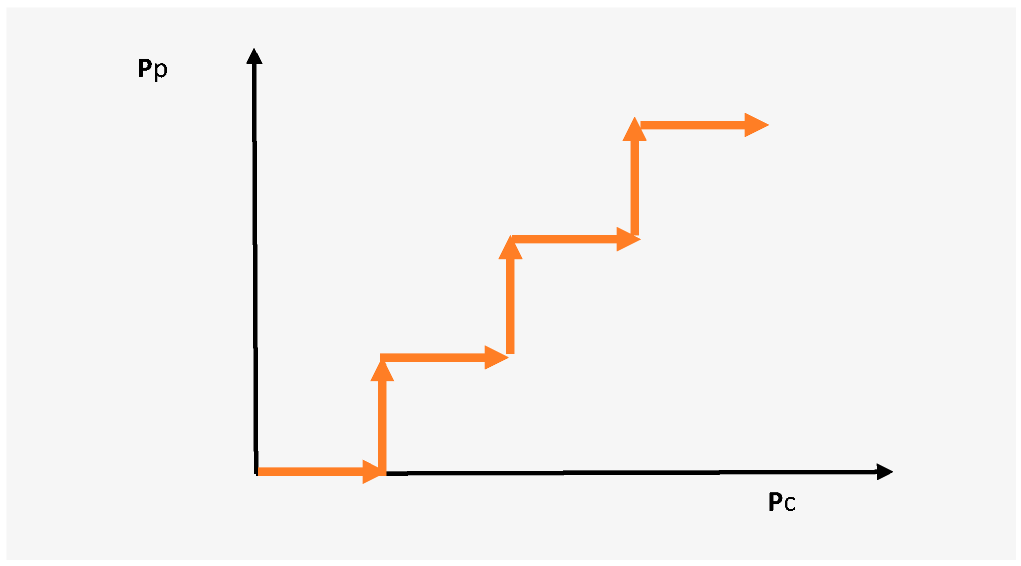
A jacketed test is conducted to measure the $K_{Jac}$. The procedure is as follows:

Firstly, the sample is put in the membrane confined by a confining pressure, $P_c$, and with no pore pressure interference. Secondly, $P_c$increases in increments while $P_p$is kept constant. In the next stage, $P_p$is increased whereas the $P_c$remains constant. This cycle is repeated with regard to the point that the confining pressure must always be larger than the pore pressure to prevent the sample from inflating like a balloon. Figure 1 demonstrates the procedure of the experiment.

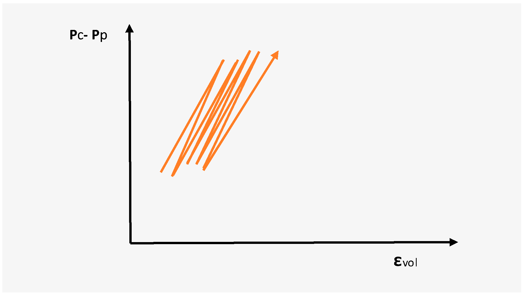
Finally, the diagram illustrating the difference between confining pressure and pore pressure, $P_c-P_p$, versus ${\epsilon }_{vol}$ is relatively similar to Figure 2.

By using fitting techniques, the matched curve for $P_c-\alpha P_p$versus ${\epsilon }_{vol}$ can be obtained (Figure 3).

$K_{Jac}$is calculated using the slope of the fitted line. $\alpha$ is also calculated from the $P_c-\alpha P_p$axis in Figure 3. Finally, the solid bulk modulus of the matrix mineral can be measured from the Equation (3).

2.1.2. Method 2

In this method, it is assumed that the rock is an isotropic material, homogeneous and has a connected porosity. In this method, Equation (3) is utilized to compute the parameter $\alpha$. Such procedure is as follows:

• Rock bulk modulus determination.

Firstly, the rock bulk modulus, K, is calculated through a jacketed test on the dry samples (on the basis of elasticity theory or acoustic velocities). The jacketed test is easy to do and there is no connection between $P_c$ and $P_p$. Then, the dry samples of the rock are subjected to loading to obtain the stress–strain chart, and calculation of the elastic moduli such as Young’s modulus or Poisson’s ratio. Then, considering the elasticity theory, rock bulk modulus is determined as

$$K=\frac{E}{3\left(1-2v\right)}.$$

(9)

where K is the rock bulk modulus (Pa), E represents the rock Young’s modulus (Pa), and v is the Poisson’s ratio. Another method to approximate the parameter K is using the propagation of sonic waves in the rock (obtained from the well log data or laboratory tests). In this method, Poisson’s Ratio, Young’s modulus, bulk modulus, and shear modulus can be calculated.

2.

Determination of bulk modulus of matrix mineral

In this case, K_m parameter can be measured with two different assumptions. If the rock is composed of a certain mineral, it is said that the rock is Mono-mineral material. For instance, in some reservoirs, the sandstone rocks are mostly made of quarts (SiO₂) mineral. Hence, parameter K_m can be reasonably assumed to be identical to the mineral bulk modulus (e.g., Quartz) as

$$K_m=K_{mono-mineral}=K_{sio2}.$$

(10)

If the rock is made of several minerals, it is said to be a multi-mineral material. Hence, in this case, the parameter $K_m$ is computed as an average value of all minerals. The lower and upper bounds of the average bulk modulus of the mineral can be estimated through Reuss and Voigt bounds, respectively. Moreover, the lower and upper bounds of the K_m can be obtained through the Hash–Strikeman bounds.

2.1.3. Method 3

In this method, it is assumed that the rock is an anisotropic material. Equation (1) is used to calculate the Biot coefficient by estimation of the bulk modulus of the rock through unjacketed test ($K_{unj}$) as

$$\alpha =1-\frac{K}{K_{unj}}$$

(11)

where α is dimensionless Biot coefficient, $K$ represents the rock bulk modulus (Pa), and K_unj indicates the mineral bulk modulus obtained from unjacketed test (Pa).

2.2. Dynamic Methods

In these methods, using the compressional and shear wave velocities, characteristics like the elastic moduli of the rock can be estimated. Computing the bulk modulus through Equation (3), we can calculate Biot coefficient.

2.2.1. Well Log Data

This method utilizes sonic log data to estimate the dynamic Biot coefficient by using the Equation (3) as

$${\alpha }_{dyn}=1-\frac{K_{dry}}{K_o}.$$

(12)

where ${\alpha }_{dyn}$ is dynamic Biot coefficient,$K_{dry}$represents the dry rock bulk modulus (Pa), and $K_o$indicates the rock effective bulk modulus (Pa).

2.2.2. Acoustic Velocity Measurement Apparatus

The basis of this apparatus is sound wave propagation in rock and measurement of the compressional and shear wave velocities. Poisson’s ratio together with elastic moduli are calculated through the following equations:

$$v_{dyn}=\frac{0.5-{\left(\frac{V_s}{V_p}\right)}^2}{1-{\left(\frac{V_s}{V_p}\right)}^2}.$$

(13)

$$E_{dyn}=\rho \frac{V_p{}^2\left(1+v_{dyn}\right)\left(1-2v_{dyn}\right)}{\left(1-v_{dyn}\right)}$$

(14)

$$K_{dyn}=\rho \left(V_p{}^2-\frac{4}{3}{V}_s{}^2\right)$$

(15)

$$G_{dyn}=\rho V_s{}^2$$

(16)

where $v_{dyn}$ represents the dynamic Poisson’s ratio, $E_{dyn}$ indicates the dynamic Young’s modulus (Pa), $K_{dyn}$ represents the dynamic bulk modulus (Pa), and $G_{dyn}$ indicates the dynamic shear modulus (Pa). The compressional and shear wave velocities are represented by the symbols of $V_p$ (m/s) and $V_s$ (m/s), respectively. $\rho$ indicates the rock density (kg/m³). Determination of shear wave velocity is always more difficult than compressional wave velocity.

Through this apparatus, one can obtain the drained and undrained bulk modulus of the samples in different radial and axial pressure and pore pressure. Hence, the Biot coefficient can be obtained as

$${\alpha }_{dyn}=(1-\frac{K_{undrained}}{K_{drained}})/B.$$

(17)

where ${\alpha }_{dyn}$ is the dynamic Biot coefficient,$K_{Undrained}$ represents the saturated rock bulk modulus under undrained condition (Pa), $K_{drained}$ indicates the saturated rock bulk modulus under drained condition (Pa), and $B$ is the Skempton coefficient.

Confining pressure has an inverse relationship with the Biot coefficient. Refs. [12,13,14] found that stress loading and confining pressure is the most important parameter in the fluid motion through the pores within the porous rocks. The in-situ stress regime also affects the pore deformations and consequently the mechanical failure of the rock [15]. This behavior is very crucial in applications such as hydraulic fracturing [16,17]. Moreover, to predict the porous rock behavior in the presence of dynamic or static loads, the active confining pressure is very crucial. Confining pressure governs the deformation of the porous rock, and its interaction with the pore fluid determines the final response of the rock to the applied stresses or forces [18,19].

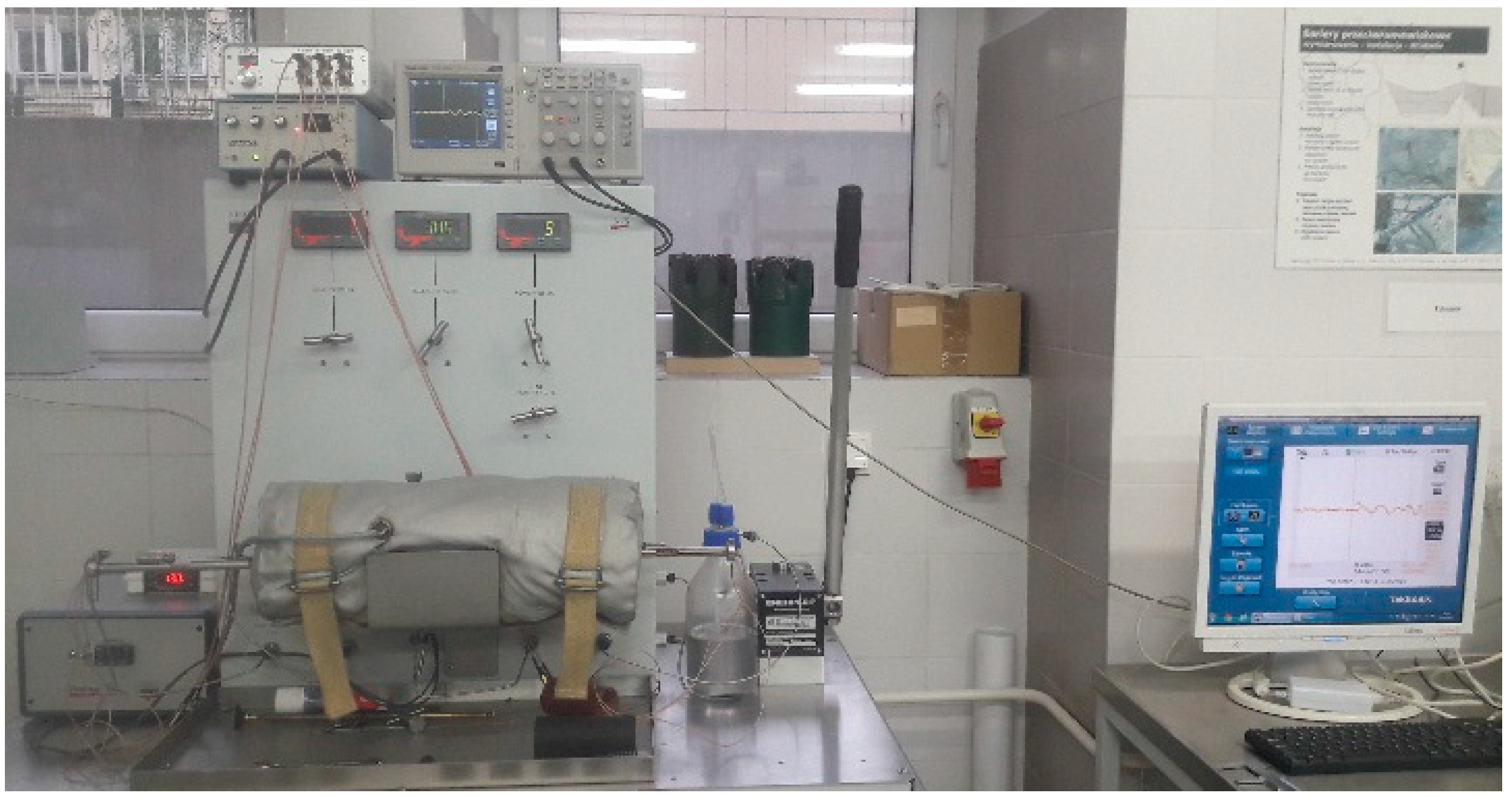
2.3. Materials

In this research, dynamic Biot coefficients of the low-porosity and high-porosity sandstone samples have been determined through the conduction of a series of non-destructive laboratory measurements. An acoustic velocity measurement apparatus (AVS) was used to measure the shear and compressional velocities of the sonic waves propagated through the sandstone specimens (Figure 4).

Before conducting the laboratory tests using the AVS apparatus, the average value of UCS for three cylindrical sandstone specimens of each category was determined.

Table 1. UCS values obtained for Low-porosity sandstone samples.

Sample Code	Diameter (mm)	Length (mm)	Massdry (gr)	UCS (MPa)
C1	38	40.5	106.2	63.45
C2	38	42	110.8	64.05
C3	38	42	110.1	53.96

and

Table 2. UCS values obtained for High-porosity sandstone samples.

Sample Code	Diameter (mm)	Length (mm)	Massdry (gr)	UCS (MPa)
H1	38	38.5	114	21.9
H2	38	40	115.2	23.95
H3	38	40.5	116.1	19.8

display the UCS results for those samples. The average UCS for low-porosity and high-porosity samples was calculated as 60.5 MPa and 21.9 MPa, respectively.

Then three different samples of each category were saturated in the saturation apparatus provided by the Laboratory of Drilling and Geoengineering, AGH University of Science and Technology. The samples were subjected 2000 Psi and 1000 Psi for low-porosity and high-porosity, respectively. After 36 hours, the samples were removed and prepared for the AVS apparatus. The properties of those samples are summarized in

Table 3. Properties of Low-porosity sandstone specimens for AVS apparatus.

Sample Code	Diameter (mm)	Length (mm)	Massdry (gr)	Masssat (gr)	Porosity (%)	Density (gr/cm3)
C4	38	43	113.5	119.25	11.80	2.64
C5	38	44.5	117.78	123.67	11.68	2.64
C6	38	45	117.62	124.10	12.70	2.64

and

Table 4. Properties on High-porosity sandstone specimens for AVS apparatus.

Sample Code	Diameter (mm)	Length (mm)	Massdry (gr)	Masssat (gr)	Porosity (%)	Density (gr/cm3)
H4	38	41	93.90	103.47	20.59	2.54
H5	38	41	93.5	103.2	20.87	2.54
H6	38	39	87.5	97.37	22.33	2.55

.

The laboratory tests were conducted on the saturated sandstone samples in both undrained and drained conditions. Because the bulk modulus of the saturated samples is larger than the drained ones, the undrained tests were conducted prior to the drained experiments. All experiments were conducted at temperature of 20°. Refs. [20,21,22,23,24] expressed that temperature can dramatically change the fluid motion and sample deformations. The reason is that the temperature changes the rheological properties of the fluid such as viscosity.

2.4. Undrained Condition

The procedure of the experimental tests in the undrained condition was so that after inserting each sample in the apparatus core holder, the confining pressure increased in increments of 200 psi regularly. When the confining pressure was raised, the pore pressure increased simultaneously. After each increment, the overall instant Skempton coefficient was continuously monitored to be approximately equal to 1. The overall Skempton coefficient was calculated as

$$B=\frac{\mathsf{\Delta }{P}_p}{\mathsf{\Delta }{P}_c}=\frac{P_{p2}-P_{p1}}{P_{c2}-P_{c1}}$$

(18)

where $B$ represents the Skempton coefficient, $P_{p2}$ and $P_{c2}$indicate the pore pressure and confining pressure at the last increment, respectively; similarly, $P_{p1}$ and $P_{c1}$indicate the pore pressure and confining pressure at the first increment, respectively. Also, at the end of each increment, the instant Skempton coefficient was calculated. At each increment, the values of pore pressure, confining pressure, P-wave and S-wave flight time, and P-wave and S-wave velocities were recorded. Then, by using the flight time, the wave velocities were computed. Afterwards, dynamic parameters including elastic moduli together with Poisson’s ratio of the sample were calculated for each $P_p$ and $P_c$ under undrained condition. 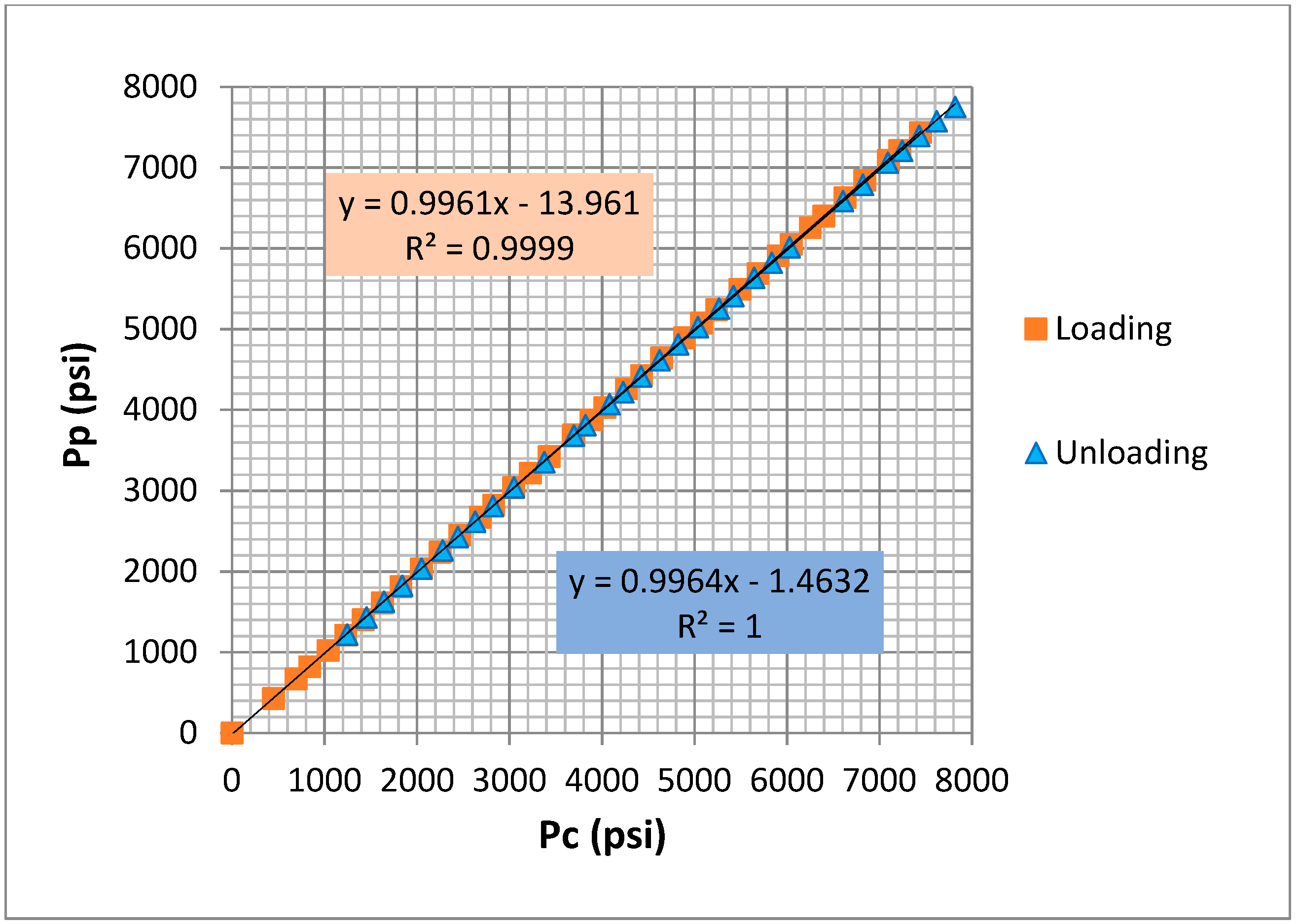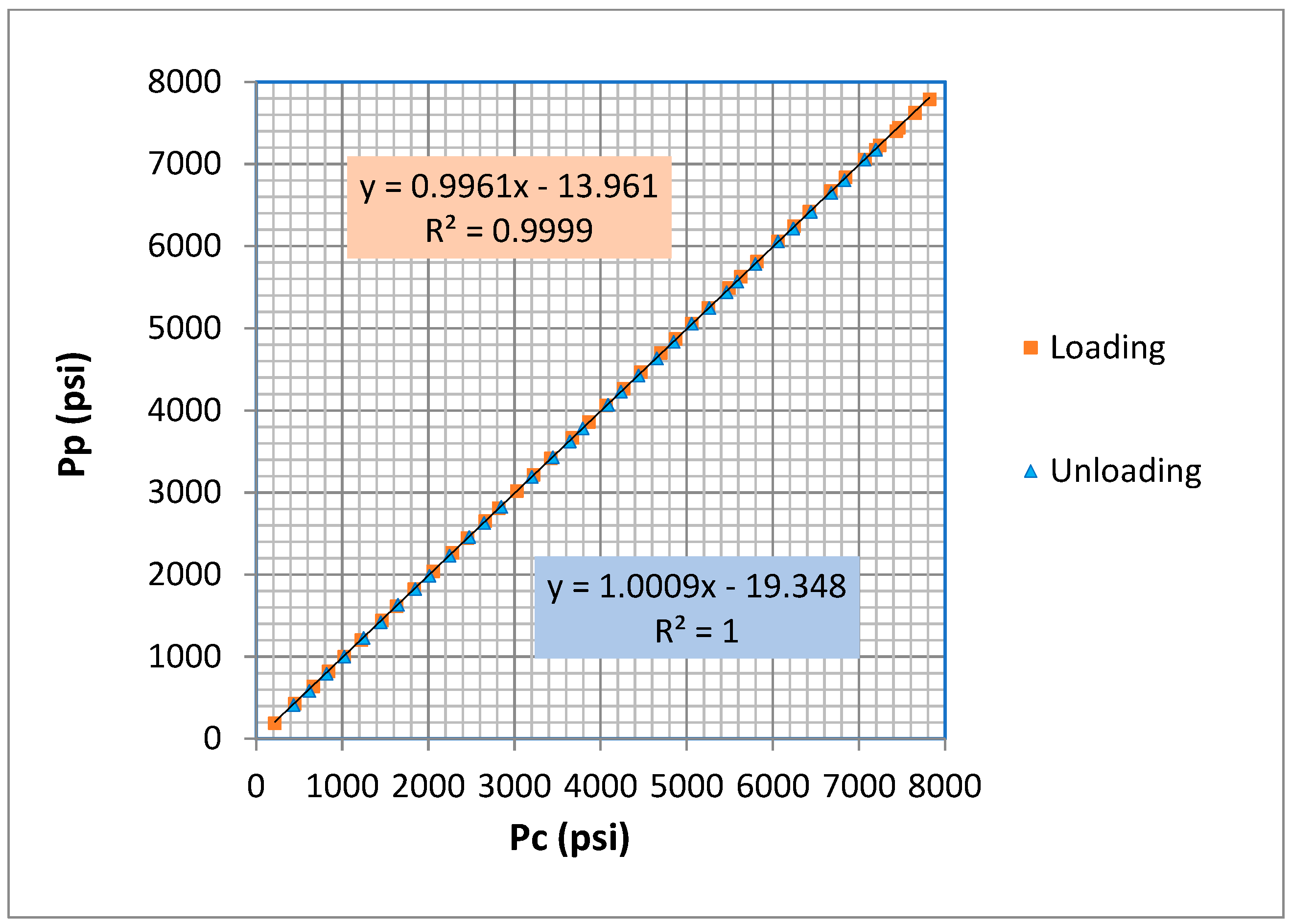When the confining pressure reached the value that pore pressure did not equally increase to compensate for, the instant B decreased. When instant B reached under 0.93, the loading stage was stopped. At this time, the overall Skempton coefficient was obtained in the range of 0.98–1 for each sample. Then, to return the sample to the initial state, the confining pressure was reduced (unloading stage) with regular increments of 200 psi until neither confining pressure nor pore pressure existed. At the end of each undrained test, the value of undrained dynamic bulk modulus was calculated through Equation (16) for each increment through the test.

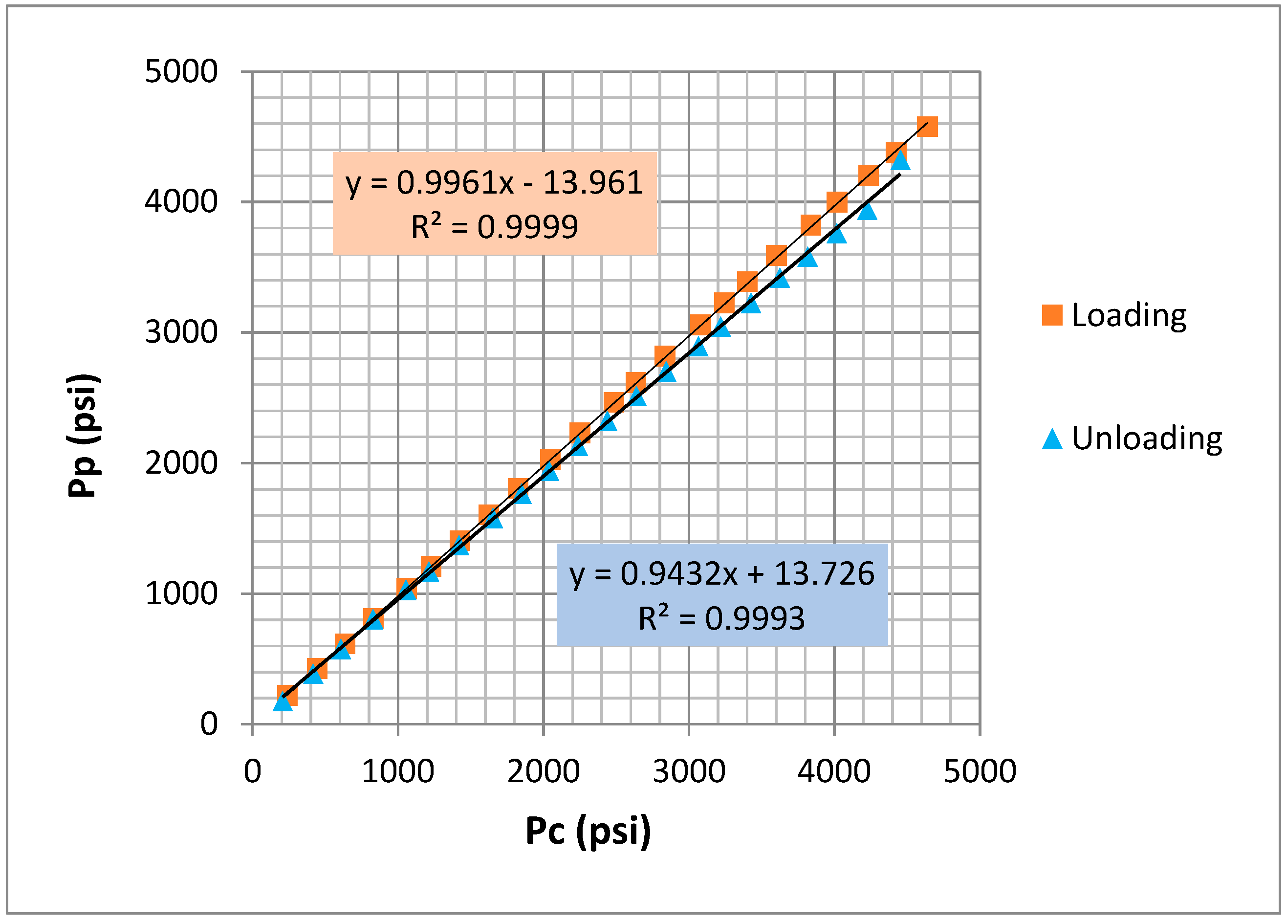
Figure 5, Figure 6 and Figure 7 illustrate the change of $P_p$ versus $P_c$ only for low-porosity samples during loading and unloading stages. Here, the aim is only to show the procedure of the undrained conditions and the change in pore pressure versus the change in confining pressure. Hence, for the prevention of repetition, only the figures related to the low-porosity samples have been presented in this section.

2.5. Drained Condition

To provide the drained condition, two valves of pore pressure on the apparatus were opened to allow the water to escape from the sample subjected to the applied confining pressure. The confining pressure was regularly increased in increments of 200 psi. At each increment, the values of pore pressure, confining pressure, compressional and shear wave, flight time, and velocities were recorded, and dynamic parameters, including elastic moduli and Poisson’s ratio, of the samples were calculated for each $P_p$ and $P_c$ under drained condition. Applying the confining pressure was continued up to the maximum confining pressure under the previous corresponding undrained test. At the end of each drained test, the drained dynamic bulk modulus of the sample was calculated through Equation (13) for each increment through the test and compared to the corresponding undrained bulk modulus of the sample under the different confining pressures. Finally, using Equation (15), the dynamic Biot coefficient was computed for each sample. 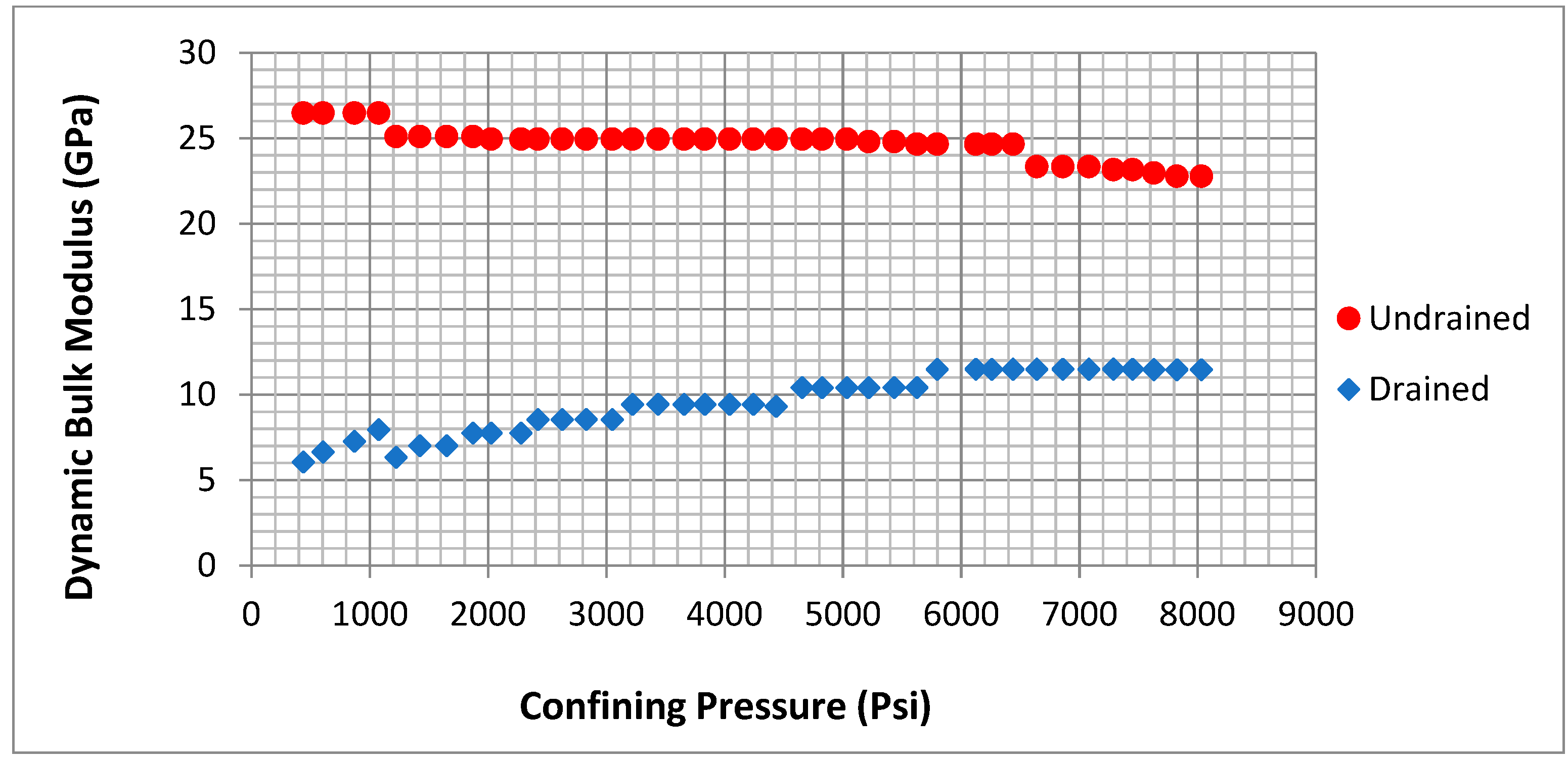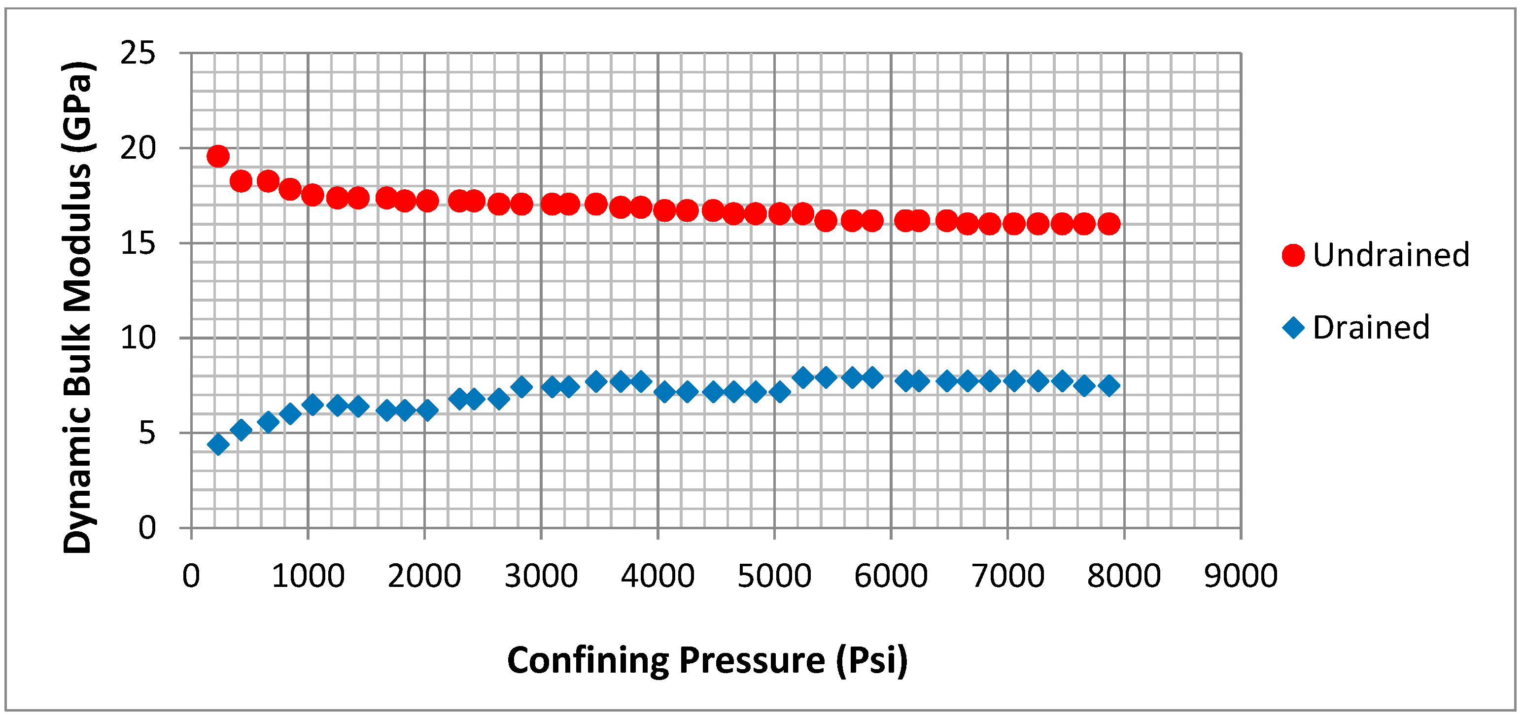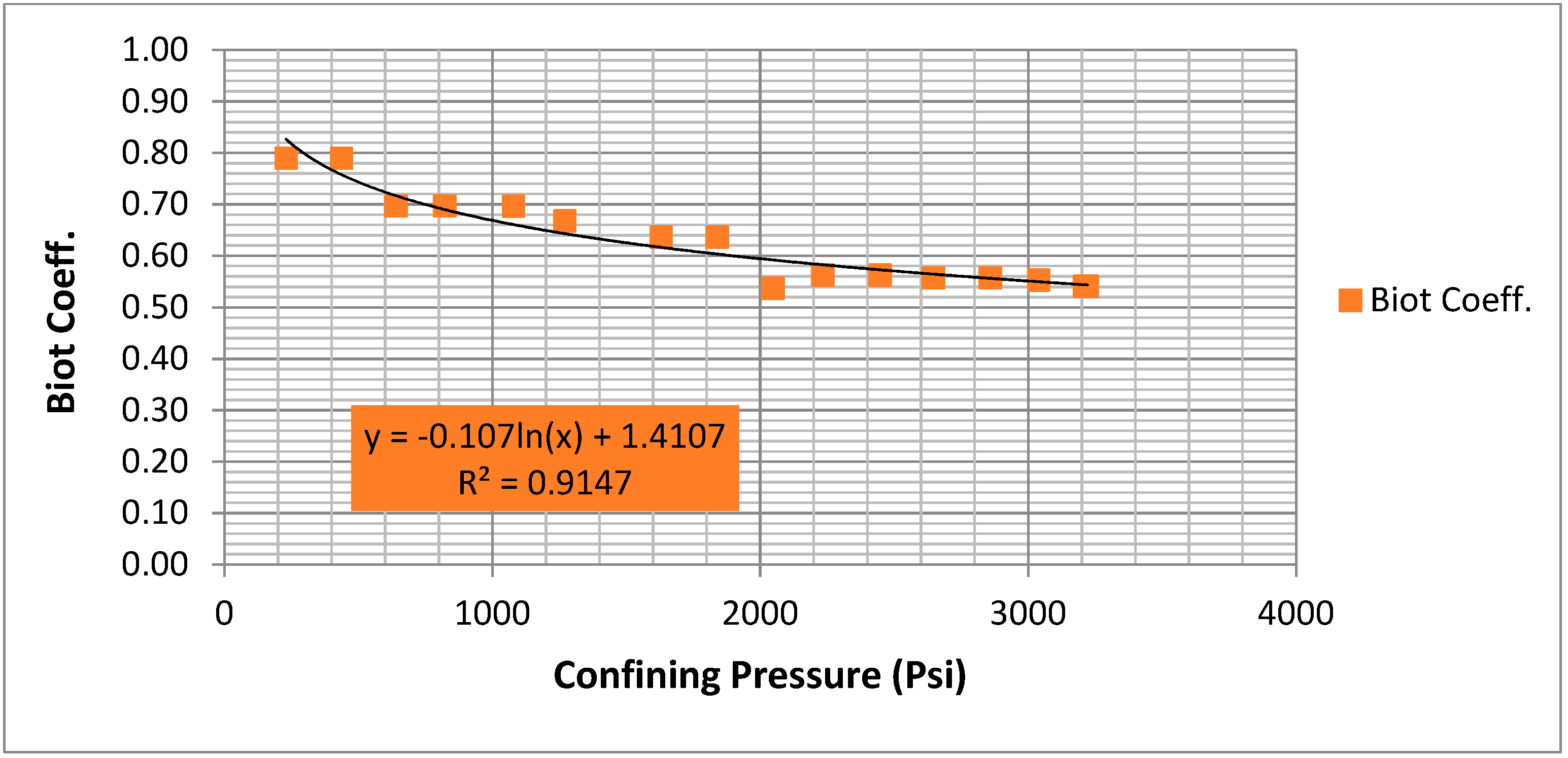Figure 8, Figure 9, Figure 10, Figure 11, Figure 12 and Figure 13 display the variation of the undrained and drained dynamic bulk moduli, and Biot coefficient with confining pressure for C4, C5, and C6 specimens.

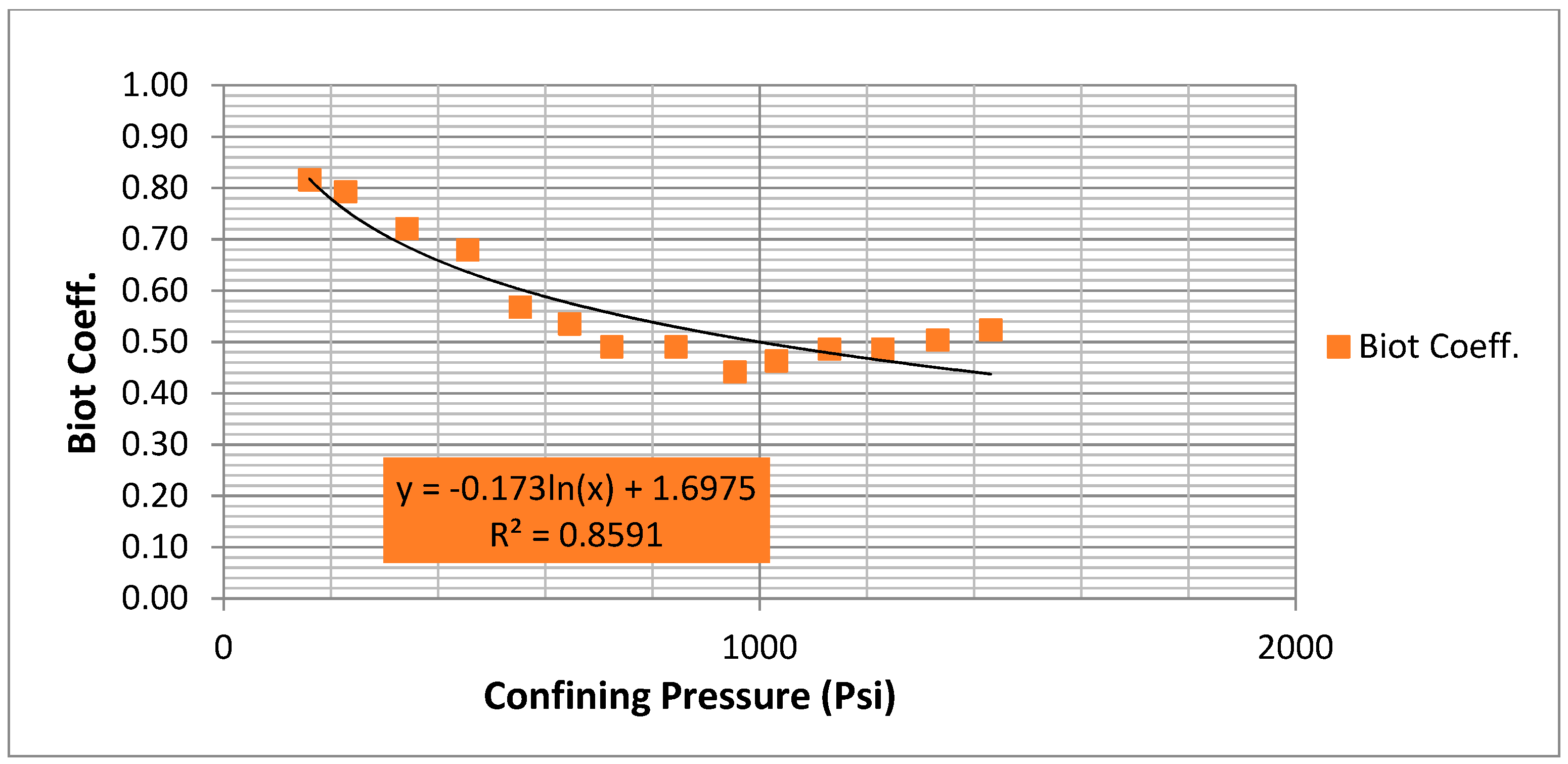
According to these results, the following empirical correlation can be developed for low-porosity sandstone samples:

$${\alpha }_{dyn}=-0.090Ln\left(P_C\right)+1.34$$

(19)

where ${\alpha }_{dyn}$ is the dynamic Biot coefficient and $P_C$ is confining pressure (psi). For low-porosity samples, the value of R-squared is around 0.91. This confirms that the obtained correlation can be developed for the same samples. It should be noted that as the average value of UCS for these three samples was equal to 60.5 MPa (≅ 8775 psi), we can observe that the confining pressure can be in the range 0–8000 psi.

Similarly, Figure 14, Figure 15, Figure 16, Figure 17, Figure 18 and Figure 19 display the variation of the undrained and drained dynamic bulk moduli and Biot coefficient with confining pressure for H4, H5, and H6 specimens.

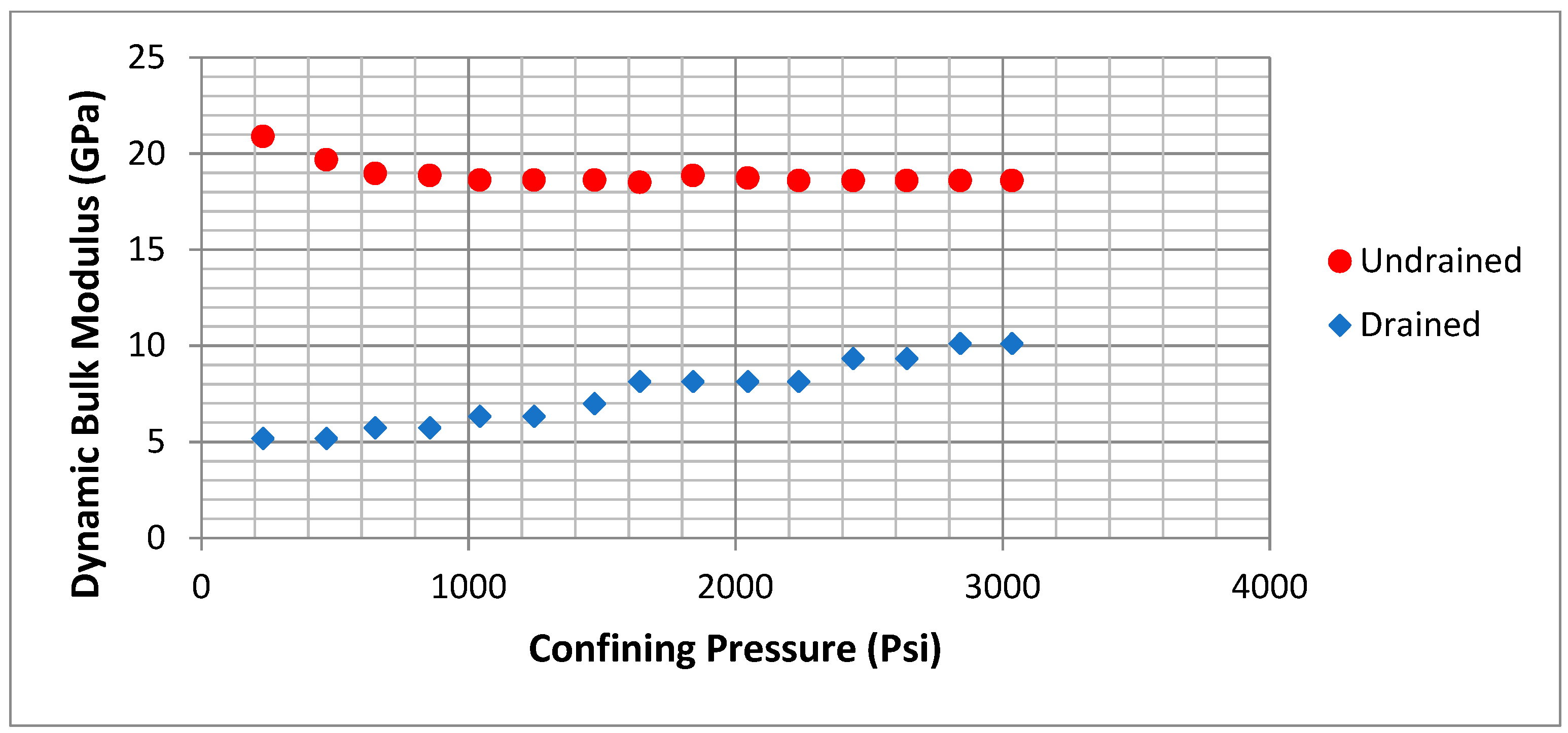
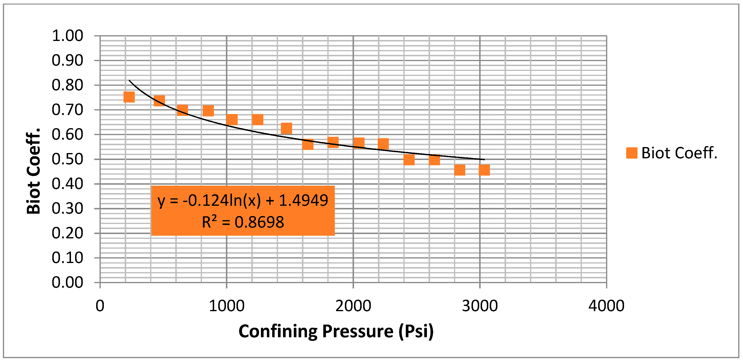
According to these results, the following empirical correlation can be developed for high-porosity sandstone samples:

$${\alpha }_{dyn}=-0.136Ln\left(P_C\right)+1.56$$

(20)

where ${\alpha }_{dyn}$ is dynamic Biot coefficient and $P_C$ is confining pssure (psi). Furthermore, the interesting point about R-squared is that it has been obtained as 0.85. Hence, it can be said that the empirical correlation can depict a reasonable value of the dynamic Biot coefficient versus confining pressure. Moreover, the average value of UCS for the high-porosity samples was equal to 21.9 MPa (≅3175 psi). From Figure 14, Figure 15, Figure 16, Figure 17, Figure 18 and Figure 19, it can be seen that the range of confining pressure can be between 0 and 3000 psi.

Comparison between the low-porosity and high-porosity samples indicates that, as the porosity increases, the Biot coefficient decreases more remarkably with confining pressure. This implies that as the pore space is larger in the sample, the effect of pore fluid on the volume change of the bulk sample is greater.

In addition, in lower confining pressures, the change of Biot coefficient is more significant when compared to the higher confining pressure near the value of UCS of the sample. At lower pressures, the dynamic drained bulk modulus of the sample increases at a substantial rate, while for the confining pressure values adjacent to the UCS, its change rate is smoother. However, the dynamic undrained bulk modulus of the sample does not change remarkably with the confining pressure. This is the reason that Biot coefficient decreases with increasing confining pressure. For high-porosity samples, the change in the dynamic undrained bulk modulus is higher in comparison to the low-porosity sandstone samples.

3. Discussion

In dynamic calculation of the Biot coefficient, compressional and shear wave velocities are the most fundamental parameters to calculate the elastic moduli of the samples. During the experiments, the ratio of compressional wave velocity to the shear wave velocity changed between 1.6–1.8 for both low-porosity and high-porosity samples. Our findings demonstrated a good agreement with the relationship between $V_s$ (m/s) and $V_p$ (m/s) introduced by [25,26] as

$$V_s=0.79\left(1-V_p\right)$$

(21)

This relationship was introduced based on investigations of the wave velocities within a number of sandstone rocks. On a positive note, when determination of the $V_s$ is difficult, one can utilize this equation as finding $V_p$ is very easy.

In this research, it was found that developing a correlation only between the porosity and Biot coefficient cannot describe the real response of the porous rock under different values of confining pressure. As in every petroleum, mining, and civil engineering project, the measurement of the rock porosity is very simple, the previous correlations are suitable for a fast estimation of the Biot coefficient. However, as the scale of the project becomes larger, the effect of confining pressure must be taken into account. For instance, when the value of confining pressure or in situ stress magnitude lies between 7 and 14 MPa, the Biot coefficient declines more remarkably in comparison to the case when the values of confining pressure are greater than 21 MPa. This relationship was introduced based on investigations of the wave velocities within a number of sandstone rocks. On a positive note, when determination of the $V_s$ is difficult, one can utilize this equation as finding $V_p$ is very easy.

The empirical correlations present an acceptable R-squared of 0.9 and 0.85 for low-porosity and high-porosity samples, respectively. This also can imply that as the porosity of the samples increases, the empirical correlations lose gradually their precision. However, sandstone samples present much better correlations when they are compared to shale specimens. Ref. [27] conducted a set of laboratory experiments on shale rocks with different porosity and confining pressure. They found that shale rocks show a very changeable Biot coefficient in different values of porosity and confining pressure. They turned out that the anisotropy of shale permeability significantly affects the measured Biot coefficient. The samples that were taken vertically from the horizontal shale layers illustrated further less Biot coefficient in comparison to the samples taken in the horizontal direction. In this study, it was found that the dynamic Biot coefficient for the sandstone samples does not depend on the direction of sampling. In spite of shale formations, sandstone layers do not show a remarkable anisotropy of permeability in different directions.

4. Conclusions

During the undrained experiments, the Skempton coefficient was kept around 1 to avoid the plastic deformations in the structure of the samples. Moreover, at the end of each increment, the instant Skempton coefficient was calculated. At each increment, the values of pore pressure, confining pressure, compressional and shear wave flight time and velocities were recorded. Using velocities, the dynamic parameters including dynamic elastic moduli as well as dynamic Poisson’s ratio were calculated for each $P_p$ and $P_c$ under undrained condition. When the confining pressure reached the value that pore pressure did not equally increase to compensate for, the instant Skempton coefficient decreased. When the instant Skempton coefficient decreased to the values less than 0.93, the experiment was stopped. At this time, the overall Skempton coefficient was mostly in the range of 0.98–1.

In this study, the average value of porosity for low-porosity sandstone samples was 11.5% while it was 21.0% for high-porosity specimens. For both samples, the following relationship between the dynamic Biot coefficient and confining pressure was obtained as

$${\alpha }_{dyn}={\{}_{-0.136Ln\left(Pc\right)+1.56;\mathit{for}\mathit{porisity}=21.0\%}^{-0.090Ln\left(Pc\right)+1.34;\mathit{for}\mathit{porisity}=11.5\%}$$

(22)

where ${\alpha }_{dyn}$ is dynamic Biot coefficient, and $P_C$ is confining pressure (psi). Furthermore, the value of R-squared for low-porosity and high-porosity samples was 0.91 and 0.85, respectively. This indicates that for lower values of porosity, the estimated value for dynamic Biot coefficient is more precise.

The results demonstrate that, under lower values of confining pressure (7–14 MPa or 1000–2000 psi), an increase in confining pressure leads to a remarkable reduction in the dynamic Biot coefficient. In fact, for this lower range of confining pressure, the dynamic Biot coefficient decrease at a much higher rate in comparison to the high values of confining pressure. In this study, dynamic Biot coefficient was calculated within the range of 0.50–0.79 and 0.52–0.84 for low-porosity and high-porosity samples, respectively.

Furthermore, our findings confirm that, as the porosity of the samples increases, the dynamic Biot coefficient reduces more significantly with confining pressure. This illustrates that, as the pore volume within the sample is higher, the influence of the containing fluid on the volume change of the bulk sample is much more noticeable.