Abstract
California has set two ambitious targets aimed at achieving a high level of decarbonization in the coming decades, namely (i) to generate 60% and 100% of its electricity using renewable energy (RE) technologies, respectively, by 2030 and by 2045, and (ii) introducing at least 5 million zero emission vehicles (ZEVs) by 2030, as a first step towards all new vehicles being ZEVs by 2035. In addition, in California, photovoltaics (PVs) coupled with lithium-ion battery (LIB) storage and battery electric vehicles (BEVs) are, respectively, the most promising candidates for new RE installations and new ZEVs, respectively. However, concerns have been voiced about how meeting both targets at the same time could potentially negatively affect the electricity grid’s stability, and hence also its overall energy and carbon performance. This paper addresses those concerns by presenting a thorough life-cycle carbon emission and energy analysis based on an original grid balancing model that uses a combination of historical hourly dispatch and demand data and future projections of hourly demand for BEV charging. Five different scenarios are assessed, and the results unequivocally indicate that a future 80% RE grid mix in California is not only able to cope with the increased demand caused by BEVs, but it can do so with low carbon emissions (<110 g CO2-eq/kWh) and satisfactory net energy returns (EROIPE-eq = 12–16).
1. Introduction
Electricity is increasingly recognised as an essential commodity to ensure the economic growth, productivity and well-being of modern societies. Ensuring a reliable supply of electricity is, therefore, of crucial importance. At the same time, it is also commonly accepted that the ever-growing demand for energy is in large part responsible for the increasing concentration of carbon dioxide (CO2) in the atmosphere [1]. This awareness has prompted many countries to approve The Paris Agreement in 2015 and to commit to the reduction of greenhouse gas (GHG) emissions to the atmosphere [2]. Among the measures implemented by governments, decarbonizing electricity generation systems has rightfully taken centre stage.
A shift to renewable energy resources is seen as the most promising strategy to reduce GHG emissions from electricity, prompting scholars and researchers to better investigate the energy implications, technical feasibility and environmental impacts of their increased use [3,4,5,6,7,8,9].
Life cycle assessment (LCA) is the de-facto standard method to fully assess the environmental impacts and the energy implications related with all the life-cycle stages of the technologies comprising the electricity grid system.
Analysing the system as a whole is important because the grid’s overall impacts depend not only on the technologies that comprise it, but also on the location, the specific electricity demand profile and the associated requirement for energy storage, as evidenced in recent analyses [10,11,12,13,14,15,16,17].
In California (USA), the government has established an ambitious plan to generate 60% and 100% of its electricity using renewable energy technologies, respectively, by 2030 and by 2045 [18]. The plan also aims to reach overall 40% and 80% reductions in GHG emissions by the same years.
Photovoltaic (PV) technologies play a significant role in future energy scenarios where a high degree of decarbonization is sought [19,20,21,22]. At the same time, strong penetration of renewable energies, and PV in particular, in the electricity grid mix will also require a parallel increase in the deployment of energy storage systems due to the inherent intermittence of these resources. The interdependence of PV and energy storage for the future of the California grid mix has been discussed elsewhere by the same authors [23].
In recent years, concerns have begun to emerge about how a rapidly increasing deployment of electric vehicles (EVs) and the associated additional demand for electricity could potentially have adverse effects on the electricity grid system, in terms of reduced stability and reliability of electricity supply, and/or worsening environmental impacts. Hoaraua and Perez refer to photovoltaic generation and electric mobility as disruptive technologies for the energy and transport sectors and claim that their interaction poses challenges that require investigations in a distribution grid [24]. Moon et al. write that an accurate prediction of the charging demand for EVs is required to ensure the stability of the power grid that will be required to effectively meet the additional electricity demand due to EV penetration in the transport sector [25]. Das et al. investigate a scenario for the future deployment of EVs and their integration with the power grid, analysing a range of ensuing issues and benefits [26]. Kasprzyk et al. emphasise the challenge of developing and implementing energy storage technologies to adapt the power grid to the needs of a growing demand for EV charging [27]. Brinkel et al. analyse the voltage fluctuations in PV electricity generation due to cloud transients and suggest a strategy to mitigate this effect based on altering the EV charging process [28]. Cheng et al. found that large-scale use of battery electric vehicles (BEVs) could actually provide benefits in terms of CO2 emission reductions at grid level [29]. In addition, Kasprzyk et al. present results according to which the use of BEVs can reduce energy losses by modifying the shape of the curve for daily load [30].
However, the literature still lacks high temporal resolution analyses of how future electricity grids featuring a high penetration of renewables would cope (from a technical as well as an environmental viewpoint) when called upon to satisfy the combined electricity demand of a large fleet of EVs plus all other utilities at the same time.
This study aims to fill this knowledge gap by building on a previously published LCA and net energy analysis (NEA) of the domestic electricity generation mix in California [23] and extending the scope of analysis to include a range of scenarios of high penetration of EVs. Consistent with the previous study, a high temporal resolution approach was retained with regards to all the underlying electricity demand and generation data.
The goal of this new study is thus two-fold: firstly, to verify, with an hourly resolution, the prospective stability and reliability of the California electricity grid in 2030, assuming that even larger quantities of renewable energies will be deployed to meet an 80% domestic renewable electricity generation target, while at the same time satisfying the combined electricity demand of all pre-existing utilities plus a planned large penetration of EVs in the transport sector. Secondly, to quantify the 2030 year-end life-cycle environmental and energy burdens associated with the electricity grid under this new set of scenario assumptions.
2. Materials and Methods
2.1. Power Dispatch Data
Historical data with 1 h resolution for electricity generation (disaggregated by technology), power curtailment for wind and PV generators, and electricity imports from out-of-state in the year 2018 were collected from the Open Access Same-time Information System (OASIS) archive of the California Independent System Operator (CAISO) [31]. These data were used as the starting point for the modelling of the future scenarios, in a similar way as previously described in the parent study [23]. For a detailed discussion of the individual energy generation technologies comprising the California grid mix, their expected future trajectories, and the way in which they were modelled, the reader is also referred to the same study. Specifically for PVs, updated assumptions have been made here, consistently with the latest literature, as detailed in Section 2.2. In addition, revised assumptions have been made on purpose-built lithium-ion batteries (LIBs) for grid-level energy storage, as explained in Section 2.3.
2.2. Photovoltaic (PV) Electricity
Solar photovoltaic (PV) energy has grown rapidly in California in the last 2 decades to address the clean energy transition challenge. In 2020, the PV power installed capacity reached approximately 32,870 MW [32], out of which approximately 20% was comprised by cadmium telluride (CdTe) thin-film installations (personal communication by First Solar, the leading producer for this technology). The remaining PV technology shares were based on the latest global production data collected in the Fraunhofer Institute for the solar energy report, which lead to 28% single-crystalline silicon (sc-Si), and 52% multi-crystalline silicon (mc-Si).
In this analysis, ground-mounted PV systems were assumed, which were composed of PV panels and balance of system (BOS), including mechanical and electrical components such as inverters, transformers and cables, as well as system operation and maintenance.
The same Fraunhofer report also provided the current PV commercial efficiencies, namely: 20.5% for sc-Si, 18% for mc-Si, and 18% for CdTe [33].
PV systems are still on steadily improving trends, and, therefore, future efficiencies were taken into account, according to the recent IEA projections [34], as follows: 23% for sc-Si and CdTe, and 22% for mc-Si.
The lifetime of PV systems was assumed to be 30 years, according to the IEA Photovoltaic Power Systems (PVPS) Task 12 guidelines [35].
In terms of material and energy utilization for the production of PV panels, there has been significant improvement over the years [36,37]. Specifically, as discussed in Fthenakis and Leccisi, 2021 [37], the main improvements in c-Si PV module production were associated with: (i) reduced wafer thickness, from 200 μm in 2015 to 170 μm (sc-Si) and 180 μm (mc-Si) in the 2020 productions; (ii) reduced kerf losses, from 145 μm for slurry-based sawing to 65 μm in 2020, using diamond cutting, and (iii) reduced electricity demand in the sc-Si and mc-Si wafer stages, which it was currently 4.76 kWh/m2 (for sc-Si) and 5.56 kWh/m2 (for mc-Si). According to the latest IEA-PVPS Task 12 LCI report [38], the current reported silicon demands were 595 g/m2 and 634 g/m2 for sc-Si and mc-Si, respectively, which were significantly lower than previous estimates (1580 g/m2 and 1020 g/m2) [39].
Accordingly, in this analysis, these most recent datasets have been considered for the PV system modelling. For c-Si PV modules, the foreground inventory was based on the latest IEA PVPS Task 12 report [38], and the life-cycle impact results were based on Fthenakis and Leccisi, 2021 [37]. CdTe PV module data were provided directly by the leading producer for this technology (First Solar), and life-cycle impacts were based on Leccisi et al., 2016 [36]. First Solar also provided information on the balance of system (BOS) for ground-mounted installations, and the same BOS data were also used for the c-Si technologies. Background life-cycle inventory data were taken from the Ecoinvent database [40] and adapted to the current geographical production conditions in order to be as accurate and realistic as possible. Specifically, the main producer country for c-Si PV panels is currently China, while CdTe is produced in the US. Their electricity grid mixes were updated according to the latest available information [41].
PV end of life (EoL) management and recycling were excluded from the analysis boundary because of the dearth of large-scale recycling facilities on which to base realistic future estimates for collection rates and large-scale material recovery. However, according to preliminary studies, the future recycling of PV components may lead to improvements in energy and environmental performance as well as economic benefits due to the high value of recycled copper, aluminium, silicon [42,43].
Finally, emerging PV technologies (e.g., single-junction and tandem perovskites) were not included in this analysis because they are not yet available at an industrial scale. However, they are expected to become available in the next years, and their penetration could further reduce the energy and environmental impacts of PV electricity, as estimated in recent perovskite LCA comparative studies [37,44,45,46].
2.3. Lithium-Ion Battery (LIB) Energy Storage
In this analysis, lithium-ion batteries (LIB) were assumed because they are considered to have the largest potential for future development and implementation [47]. They also show potential benefits in terms of economic cost, charge capability, energy density and efficiency. A number of different cathode types have been used in Li-ion batteries, with varying chemical compositions such as lithium manganese oxide (LMO = LiMn2O4), lithium iron phosphate (LFP = LiFePO4), lithium cobalt oxide (LCO = LiCoO2), lithium nickel-manganese-cobalt oxide (NMC or NCM = LiNixCoyMnzO2), lithium nickel-cobalt-aluminium oxide (NCA = LiNiCoAlO2). Among the alternatives, LMO and LFP batteries are considered the least environmentally critical because they are not based on toxic or rare metals such as cobalt. An earlier LCA study focused on PV complemented with LIB storage performed a sensitivity analysis comparing LMO with LFP alternatives [48], and the results showed small changes in both energy and carbon emissions impacts. Thus, in this analysis, the model assumes 100% LIB based on LMO cathode composition, which has been modelled using the Ecoinvent database [40].
A crucial factor to be determined was LIB lifetime because it affects the rate at which batteries are replaced in a system, which has relevant environmental, energy and economic implications, as discussed in Peters et al., 2021 [49]. Previous studies reported ranges between 10 and 30 years for dedicated first-life battery lifetimes and approximately one full cycle per day [49,50,51,52,53]. Different reported ranges reflect the complexity of estimating the battery ageing process, which results in a capacity fade and an increase of inner resistance. In this analysis, a 20-year LMO lifetime has been assumed as a baseline, which is the average of previous estimates (this value may still be considered conservative for future scenarios since battery lifetime is expected to increase further). To address the uncertainty on this critical parameter, a sensitivity analysis has been performed, considering a lifetime range from 10 to 30 years.
2.4. Additional Electricity Demand for EVs
California state policies for the reduction of CO2 emissions are comparatively aggressive, and executive order B-48-18 established a target of 5 million Zero Emission Vehicles (ZEVs) by 2030, while executive order N-79-20 established that 100% of in-state sales of new passenger cars and trucks shall be zero-emission by 2035. Given that battery electric vehicles (BEVs) are widely regarded as the most promising ZEV technology in the medium-to-long term, in this study, the simplifying assumption was made that all future light-duty ZEVs in California will be BEVs. Based on executive order B-48-18, it was then estimated that the whole California light-duty vehicle (LDV) fleet in 2030 would include at least 5 million BEVs, and that, in more ambitious scenarios for the same year, the number of light-duty BEVs could possibly be as high as 10 million (cf. Section 2.5).
The California Energy Commission is the primary state agency responsible for managing and developing the electricity grid and for planning the energy policies in California. The commission uses various data resources to forecast and assess the energy demand and to create the energy system for the future to guarantee prosperity for the nation. One such source of data is the California Vehicles Survey, which is used to assess current and future vehicle ownership in California in the residential and commercial LDV sectors, subdivided into 13 vehicle segments by size and type, ranging from subcompact cars to full-size vans.
It was assumed that the overall LDV fleet data reported in the survey for the years 2015–2017 [54], in terms of segment composition and kilometres travelled per year by each vehicle within each segment, will also apply to the BEVs that will form part of the fleet in 2030, with the further assumption that the total number of BEVs will be equally split between the residential and commercial sectors.
Further, Kiani et al. reported that 87% of the total distance travelled by a BEV in California was typically for intracity trips (i.e., within a city), while only 13% was for intercity travel (on highways) [55]. Assuming that these percentages will still hold for 2030, they were then combined with fuel economy information deducted from Jung et al. [56], who linearly correlated BEV mass and electricity consumption under highway and city driving conditions and the average BEV mass within each segment, which was extracted from the 2018 EPA Automotive Trends Report [57]. This enabled the calculation of the cumulative demand for electricity for the entire BEV fleet in 2030.
The 2015–2017 California Vehicles Survey also provided an additional questionnaire for residential and commercial BEV owners, where it was asked to select a time in the morning, in the afternoon, in the evening and in the night on a typical weekday when they would normally charge their vehicles’ batteries [54]. Based on the resulting charging times data, it was thus possible to create a typical daily BEV charging profile with an hourly resolution, which was assumed to apply equally to all days of the year (specific information on vehicle charging at weekends and bank holidays was not available). This charging profile was then used to calculate the hourly power demand for all BEVs in 2030.
For full transparency, all the detailed data and calculations on BEVs are reported in the Supplementary Materials.
Finally, the manufacturing, maintenance and end-of-life treatment of BEVs were excluded from this assessment since they fell outside of the intended scope of the study, which focuses on quantifying the life-cycle environmental and energy burdens associated with California’s domestic electricity supply, under a range of scenarios characterised by varying degrees of penetration of BEVs.
2.5. Definition of Future Scenarios for 2030
The total California in-state generation in 2018 was 165 TWh, to which non-renewable energy technologies contributed by 50% (out of which 39% was gas and 11% nuclear), and renewables comprised the remaining 50% (16% PV, 15% hydro, 10% wind, 5% geothermal, 3% biomass and 1% Concentrating Solar Power (CSP)).
As discussed in Raugei et al., 2020 [23], PV may be expected to be singularly relied upon to raise the share of renewable energy generation in the California domestic grid mix to 80% by 2030, with a parallel growth in energy storage. In addition, by 2030, it is expected that all nuclear reactors will have been decommissioned and that gas-fired generation will be curbed, in accordance with the government’s plan to minimise GHG emissions. Even so, gas-fired electricity will continue to play an important role as a dispatchable technology to follow the demand profile and to help compensate for the intrinsic intermittency of wind and solar energy. The generation profiles for hydro, biogas, biomass, geothermal, wind and CSP are instead assumed to remain the same as in 2018.
Five future scenarios for California in 2030 have been considered in this study.
The first one, referred to as “BAU” (business as usual), is a counterfactual with no penetration of BEVs. In this scenario, the total annual electricity demand is expected to remain at 226,342 GWh (i.e., the same as in 2018). The high temporal resolution grid balancing model (cf. Section 2.6) then indicated that the 80% domestic renewable energy generation target (%RE target) could be achieved with approximately 43,000 MW of installed PV power and 154,000 MWh of LIB storage capacity, i.e., equal to 60% of the PV power for 6 h. For a 100-MW PV system with an inverter loading ratio = 1.3, the inverter size must be 77 MW AC (100 MW/1.3). Using the inverter/storage size ratio (1.67) suggested by NREL [58], the storage power capacity must be 46 MW AC (77/1.67). Thus, to match a 100-MW PV system, the storage power capacity must be 60 MW DC (46 × 1.3). This also leads to 2.5% of the total variable renewable energy (VRE) generation being curtailed in this first scenario.
In the second scenario, named “Low BEV”, 5,000,000 BEVs are assumed to be present in the LDV fleet by 2030, and the total annual electricity demand is thus increased by 12%, to over 250,000 GWh. In this scenario, approximately 50,000 MW of installed PV power with 6 h of dedicated storage capacity would suffice to meet the same 80% RE target, but a 4.5% VRE curtailment would ensue.
The third scenario, named “High BEV”, sees the number of BEVs in the fleet rise to 10,000,000, and the total annual electricity demand grows further to over 280,000 GWh. In this scenario, over 60,000 MW of installed PV power with 8 h of storage would be required to meet the 80% RE target while at the same time preventing %VRE curtailment from increasing to unacceptable levels (with this combination of PV power and storage capacity, %VRE curtailment is limited to 2%).
The fourth scenario, named “High BEV DSM”, was the same as the third one, except for a new assumption being introduced about the BEV charging pattern. In this scenario, the latter is supposed to be demand-side managed (DSM) to mitigate the associated electricity demand during the night and redistribute it to the central hours of the day, the goal, of course, is to reduce the mismatch between BEV-induced demand and PV generation. Figure 1 shows the two daily EV charging patterns, the first one (continuous line) based on historical data (cf. Section 2.4) and the second one (dashed line) “flattened” by DSM. In this scenario, the 80% RE target could be met with only slightly increased installed PV power but significantly reduced deployment of dedicated LIB storage (6 h instead of 8 h); the ensuing %VRE curtailment would, however, be marginally higher at 4.4%.
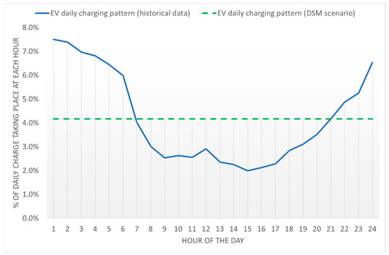
Figure 1.
Daily EV charging patterns. Solid line = historical data (scenarios 2 and 3); dashed line = with demand side management (scenarios 4 and 5).
Finally, the fifth scenario, named “High BEV DSM + V2G”, is a variation on the fourth one, in which vehicle-to-grid (V2G) technology is assumed to be rolled out, to supply a quarter of the total storage capacity. This enables energy to be pushed back into the power grid from the batteries of EVs when the latter are connected for charging. This would allow reverting to the same installed PV power as in the “High BEV” scenario, and, significantly, to further reduce the number of purpose-built LIBs, while still ensuring the availability of the same 6 h of total storage depth. In this scenario, the overall %VRE curtailment would drop to 2.0%. Furthermore, a parametric analysis was carried out to evaluate the additional degree of battery cycle ageing that this level of V2G engagement would cause to the BEV fleet. Assuming that only half of the BEVs in the fleet (i.e., 5,000,000 units) would participate in the V2G scheme, and based on an average battery capacity of 112 kWh, the resulting mean V2G battery utilization rate would be 13.6% (increasing to 27.2% if only a quarter of the BEVs participated). These results indicate that this level of V2G engagement is not likely to be detrimental to the service life of the EV batteries. Accordingly, a simple cut-off rule was adopted in the model, whereby the energy and environmental impacts associated to the manufacturing of the EV batteries were entirely attributed to their primary function of providing traction energy storage to the vehicles (and, therefore, the secondary V2G energy storage function is assumed to be impact-free).
Table 1 reports the key parameters that define the five analysed scenarios as described above.

Table 1.
Key parameters defining the five analysed scenarios for California in 2030.
Table 2 reports the resulting composition (net generation post-curtailment and storage) of the domestic California grid mix in 2030, in the five analysed scenarios.
Table 2.
Technology shares (net generation post-curtailment and storage) of the domestic California grid mix in 2030, in the five analysed scenarios. All values rounded to the nearest 1%.
2.6. Grid Operation Model
From a modelling perspective, consistently with a previous study by the same authors [23], the following approach and assumptions were adopted here to model the future California electricity grid mix in 2030 in all scenarios:
- The total hourly demand profile in 2030 for Scenario 1 (i.e., with the exclusion of the additional demand for EVs) was assumed to be the same as in 2018. This extrapolation is supported by the data for the past 19 years [31].
- The potential variations in electricity demand, in terms of both hourly profile and total year-end cumulative value, due to the large-scale deployment of BEVs in Scenarios 2 to 5 were estimated separately, as described in Section 2.4.
- Natural gas combined cycle (NGCC) output and electricity imports were assumed to be used, in synergy with LIB energy storage, to balance the hourly supply and demand curves. The hierarchical dispatch order depends on whether, at any given time, fully tapping the total potential PV generation would lead to an over- or an under-supply of electricity, vs. the demand curve. The grid balancing model relies on hourly resolution data. As such, it may fail to capture shorter-term, higher-frequency mismatches between supply and demand. However, these were not deemed to be large enough to significantly affect the overall reliability of the results. Specifically:
- (a)
- When excess PV power is available, curbing gas-fired electricity is the preferred option, as this achieves the largest reduction in carbon emissions since NGCC have the highest carbon intensity of all the technologies in the domestic grid mix and is also higher than the average grid mix of technologies used for the production of imported energy in California [59]. Then, if necessary, after cutting NGCC output all the way down to zero, electricity imports from out of state can be cut. Thirdly, if the residual potential PV output still leads to an over-supply of electricity, the excess PV electricity can be routed into storage, as long as neither the maximum storage power (P) nor the available residual storage capacity (E) is exceeded. Finally, PV curtailment would occur as a last resort.
- (b)
- Conversely, when not enough PV power is available (e.g., at times of increased demand for EV charging and reduced solar irradiation), the first strategy is to tap the available battery storage (which, however, is once again limited in terms of maximum power throughput, P). NGCC are then called upon to supply the balance, as long as doing so does not exceed the available NGCC installed power. Finally, in the rare instances when the latter condition cannot be met, the remaining demand deficit is met by increasing imports. This reversed order of dispatch is chosen to avoid potentially problematic surges in demand for imported electricity, which may be problematic or costly to fulfil.
It is noteworthy that the data collected and analysed in this study show that in California, the electricity supply-demand mismatch is potentially more pronounced in the spring months rather than, as might have been expected, in the summer. This is explained by fact that the increased electricity demand for air conditioning in the hotter summer months tends to occur at times of maximum insolation, and hence PV output, thus improving the match between supply and demand. Figure 2, Figure 3, Figure 4 and Figure 5 illustrate the sum of the contributions of the individual electricity generation profiles and the demand for the month of April, taken as a worst-case of supply-demand mismatch, for the considered scenarios. From bottom to top: green line = other renewables (i.e., the sum of hydro, biogas, biomass and geothermal); blue line = wind; yellow line = solar (PV + CSP) potential pre-storage and curtailment; grey line = demand profile excluding EV demand; black line = total demand profile.
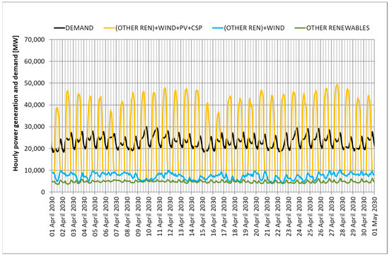
Figure 2.
Projected hourly electricity demand and potential generation (i.e., pre-curtailment and storage) for the month of April 2030, in the “BAU” (business as usual) scenario.
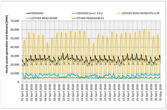
Figure 3.
Projected hourly electricity demand and potential generation (i.e., pre-curtailment and storage) for the month of April 2030, in the “Low BEV” scenario.
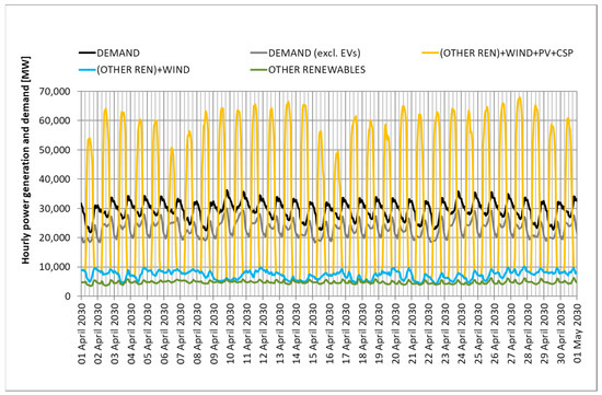
Figure 4.
Projected hourly electricity demand and potential generation (i.e., pre-curtailment and storage) for the month of April 2030, in the “High BEV” scenario.
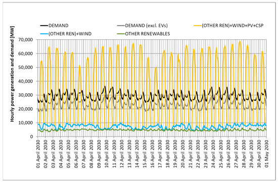
Figure 5.
Projected hourly electricity demand and potential generation (i.e., pre-curtailment and storage) for the month of April 2030, in the “High BEV DMS” and “High BEV DMS + V2G” scenarios.
2.7. Methods of Analysis
2.7.1. Life Cycle Assessment (LCA)
Life cycle assessment (LCA) is a widely applied method to assess the environmental impacts of products and processes. It takes into account all the life cycle, including raw material extraction, transport, manufacturing, use, and end of life. It has a high degree of standardization [60,61], and it benefits from well-established inventory databases, such as Ecoinvent [62], which has been used here for this assessment.
The LCA method enables the calculation of a large number of impact indicators; this paper focuses on the calculation of the global warming potential (GWP), using Intergovernmental Panel on Climate Change (IPCC)-derived characterization factors with a time horizon of 100 years and expressed in units of kg of CO2-equivalent for all gaseous emissions with the exclusion of biogenic CO2.
In addition, the cumulative energy demand (CED) and the non-renewable cumulative energy demand (nr-CED), which are life-cycle energy metrics to, respectively, quantify the total amount of primary energy directly and indirectly harvested from the environment per unit of electricity output, and the non-renewable share thereof, are calculated here, and the results are expressed in MJ of oil-equivalent per kWh (or per MJ) of electricity [63].
Finally, the life-cycle primary-to-electric energy conversion efficiency of the whole grid mix (ηG) is equal to the reciprocal of its CED:
ηG = 1/CEDG
2.7.2. Net Energy Analysis (NEA)
Net energy analysis (NEA) [64] provides a method to quantify the amount of energy “profit” from the point of view of the end-user, and its main indicator is the energy return on (energy) investment [65], defined as follows:
EROI = Out/Inv
However, NEA does not have a high degree of standardisation, and this has led to many inconsistent comparisons [66,67].
In this study, in order to integrate the LCA and NEA approaches [10,12,13,15,17], when the EROI of electricity is calculated, all the energy investments at the denominator are accounted for in terms of their respective life-cycle CED, and they are expressed in units of oil-equivalent.
When the EROI numerator is measured as the amount of electricity delivered, a subscript “el” is used (i.e., EROIel). Alternatively, when the EROI numerator is expressed as “primary energy equivalent”, a subscript “PE-eq” is used (i.e., EROIPE-eq), where:
EROIPE-eq = EROIel/ηG
It is noteworthy that the values of EROIel and EROIPE-eq become closer and closer as the primary-to-electric energy conversion efficiency of the grid mix as a whole improves. This is consistent with the replacement logic that underpins the definition of “primary energy equivalent”; in fact, asymptotically, if a grid mix is achieved ηG = 1, then one unit of electricity would be equivalent to one unit of primary energy.
3. Results and Discussion
3.1. Impacts per Unit of Electricity Delivered in 2030
The main LCA results are shown in Figure 6 and Figure 7, respectively, in terms of GWP and nr-CED per kWh of electricity delivered by the California domestic grid mix in 2030, according to the five scenarios defined in Section 2.5.
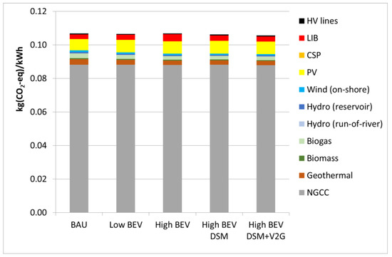
Figure 6.
Global warming potential (GWP) of 1kWh of electricity supplied by the domestic grid, with contributions by technology.
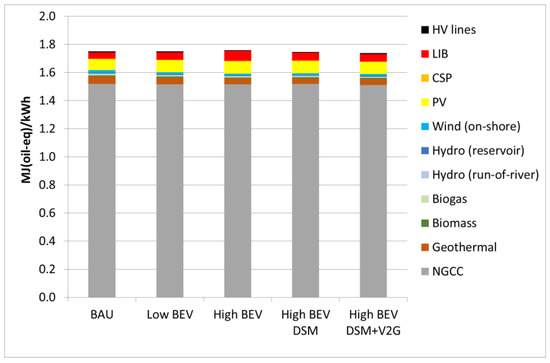
Figure 7.
Non-renewable cumulative energy demand (nr-CED) of 1kWh of electricity supplied by the domestic grid, with contributions by technology.
Comparing across the five scenarios shows that the chosen grid adaptation strategy to cope with the increased electricity demand due to BEVs, based on ramping up PV installed power and LIB battery storage, is not only technically effective at ensuring the continued matching of the total hourly demand profile (regardless of the specific number of BEVs or their charging pattern), but it also manages to do so without any appreciable adverse effect in terms of carbon emissions or non-renewable primary energy intensity. It is also noteworthy that despite the grid mix being heavily tilted towards PV (which represents between ~50 and ~60% of the total net generation in all scenarios), the largest contribution by far (~80%) to both types of impact is still caused by gas-fired electricity (which is called upon to deliver ~20% of the total electricity). Conversely, LIBs are only responsible for a very minor share of the total impacts, even in the “High BEV” scenario in which they are required in the largest quantity.
Further, Figure 8 shows that the overall life-cycle primary-to-electric energy conversion efficiency of the whole grid mix (ηG) is also remarkably stable across all scenarios, with, in fact, a very slight improvement in those scenarios with the largest penetration of BEVs. This latter effect is a direct consequence of the further increase in PV’s share of the total net generation (see Table 2), and it happens in spite of the increased demand for storage. It is worth noting that those projected life-cycle grid efficiencies values are about 1.5 to 2 times higher than the current values for California and for most other commonly assumed electricity mixes based on thermoelectric technologies [12,13,37,68].
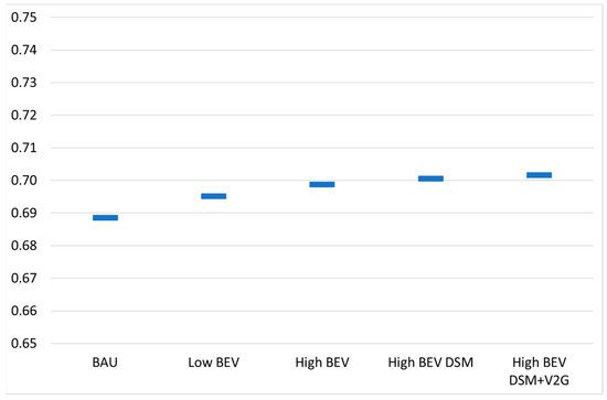
Figure 8.
Life-cycle primary-to-electric energy conversion efficiency of the domestic grid mix (ηG).
Moving on to the NEA results, Figure 9 reports the total primary energy investment required per unit of electricity delivered by the domestic grid. It is important to remember how this differs from both CED and nr-CED, in that it does not include the primary energy directly harvested from nature and then converted into electricity (e.g., the solar energy captured by the PV panels and the natural gas extracted from the earth), but only the additional primary energy invested along the supply chains (e.g., to manufacture and maintain the PV systems, and to extract and deliver the natural gas and to manufacture and maintain the NGCC power plants). From this point of view, the impacts of PVs and LIBs are then much larger, and in fact, when considered together, they represent the largest relative contribution (~50%) to the total energy investment.
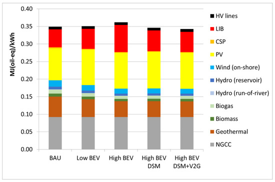
Figure 9.
Primary energy investment required per kWh of electricity supplied by the domestic grid, with contributions by technology.
Given the relatively large contribution of LIBs to the primary energy investment per kWh of electricity, a sensitivity analysis was performed on these results, by altering the assumed lifetime of the purpose-built battery packs designed for grid storage applications to cover a range from a minimum of 10 years (worst case) to a maximum of 30 years (best case), as discussed in Section 2.3. This leads to a corresponding range of EROIPE-eq values for each scenario, as illustrated in Figure 10, where the square symbol indicates the value resulting from the “baseline” lifetime assumption of 20 years.
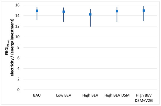
Figure 10.
Energy return on investment (EROIPE-eq) of electricity supplied by the domestic grid, with sensitivity analysis to Li-ion battery lifetime (baseline = 20 years, worst case = 10 years, best case = 30 years). The PE-eq conversions are based on the grid efficiencies reported in Figure 5 (~0.7).
Despite the increased sensitivity of the NEA indicators to the differences between the individual scenarios, and to the underlying assumption on battery lifetime, it is, however, important to always keep the necessary sense of proportion when interpreting these results, too. In fact, here too, the main message has to be that, irrespective of the exact EROIPE-eq value (which may range from ~12 to ~15.5 depending on the specific BEV deployment scenario and LIB lifetime), the California domestic gid mix in 2030 can still be expected to be characterised by a reassuring net energy performance.
3.2. Cumulative Impacts, Including Operation of 10 Million LDVs, in 2030
After finding how the carbon and energy performance of the future domestic electricity supply mix in California is unlikely to be significantly affected by the increased demand caused by a large-scale deployment of electric vehicles, it was deemed important to also look at the cumulative impacts occurring in the year of analysis across all five scenarios. The purpose of this second comparison was to highlight the extent of the benefits brought about by the replacement of internal combustion engine vehicles (ICEVs) with EVs while changing the functional unit of the assessment to the total electricity delivered by the California domestic grid, plus the use phase of a fleet of 10 million LDVs. In order to do so, the use-phase carbon emissions of ICEVs were estimated on the basis of the 2020 EPA Automotive Trends Report [69], which provides CO2 emission data per vehicle type under highway and city driving conditions.
The resulting cumulative GHG emissions and demand for non-renewable primary energy are illustrated in Figure 11 and Figure 12, respectively. As can be seen, the replacement of 5 million (in the “Low BEV” scenario) and 10 million (in all the “High BEV” scenarios) ICEVs with corresponding numbers of BEVs leads to significant reductions in both types of impact (respectively, approximately −30% and −60%), in spite of the ensuing increase in electricity demand. This indicates that BEVs do represent an effective strategy to curb carbon emissions and reduce California’s dependency on non-renewable energy resources.
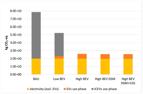
Figure 11.
Cumulative greenhouse gas (GHG) emissions of domestic electricity supply to all non-transport sectors (yellow) + use phase of a 10 million LDV fleet. “BAU” = 10M ICEVs (grey); “Low BEV” = 5M ICEVs (grey) + 5M BEVs (orange); “High BEV,” “High BEV DMS” and “High BEV DMS+V2G” = 10M BEVs (orange).
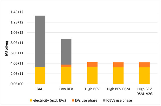
Figure 12.
Non-renewable cumulative energy demand (nr-CED) of domestic electricity supply to all non-transport sectors (yellow) + use phase of a 10 million LDV fleet. “BAU” = 10M ICEVs (grey); “Low BEV” = 5M ICEVs (grey) + 5M BEVs (orange); “High BEV,” “High BEV DMS” and “High BEV DMS+V2G” = 10M BEVs (orange).
4. Conclusions
This paper presents the results of a prospective assessment of the future carbon intensity and energy performance of electricity generation in California, based on a novel approach that leverages detailed historical hourly power dispatch data, combines them with key assumptions based on current grid decarbonization policy and electric vehicle deployment, and feeds them to a bespoke grid balancing algorithm to calculate the required amounts of PV energy and battery storage to ensure the stable operation of the grid. The grid’s ensuing carbon intensity and demand for non-renewable primary energy are then calculated using the latest life-cycle inventory data on all the technologies that comprise it (with suitable assumptions on their future trajectories). Results have shown that a future 80% renewable grid mix in California may not only be expected to be able to cope with the increased demand caused by a significant increase in electrical mobility, but also to do so with remarkably stable environmental and net energy performance, irrespective of the specific assumptions on the number of electric vehicles, their charging pattern, and on battery lifetime. In addition, the assessment of the operation of the entire domestic electricity grid plus a fleet of 10 million light-duty vehicles in 2030 has shown incontrovertibly that replacing internal combustion engine vehicles with electric vehicles, while at the same time decarbonizing the grid mix by ramping up PV and battery storage, is a very effective combined strategy to significantly curb California’s cumulative carbon emissions and non-renewable primary energy demand.
Supplementary Materials
The following are available online at https://www.mdpi.com/article/10.3390/en14165165/s1, BEV data and calculations.xlsx.
Author Contributions
Conceptualization, M.R. and A.P.; methodology, M.R.; software, M.R. and A.P.; validation, M.R., A.P., E.L. and V.F.; formal analysis, M.R.; investigation, M.R. and A.P.; resources, M.R., A.P. and E.L.; data curation, M.R., A.P. and E.L.; writing—original draft preparation, M.R., A.P. and E.L.; writing—review and editing, M.R. and V.F.; visualization, M.R.; supervision, M.R. and V.F. All authors have read and agreed to the published version of the manuscript.
Funding
This research received no external funding.
Data Availability Statement
Publicly available datasets were analyzed in this study. This data can be found here: https://www.caiso.com/TodaysOutlook/Pages/default.aspx (accessed on 19 June 2020), and here: https://www.epa.gov/automotive-trends/download-automotive-trends-report#Full%20Report (accessed on 19 June 2020). Further data presented in this study are available in the Supplementary Materials file “BEV data and calculations.xlsx”.
Conflicts of Interest
The authors declare no conflict of interest.
References
- Ritchie, H.; Roser, M. CO2 and Greenhouse Gas Emissions. Our World in Data. Available online: https://ourworldindata.org/co2-and-other-greenhouse-gas-emissions#global-warming-to-date (accessed on 19 June 2020).
- Dejuán, Ó.; Lenzen, M.; Cadarso, M.Á. (Eds.) Environmental and Economic Impacts of Decarbonization: Input-Output Studies on the Consequences of the 2015 Paris Agreements, 1st ed.; Routledge: Abingdon, UK, 2018; p. 402. [Google Scholar]
- Sørensen, B. Energy and resources. Science 1975, 189, 255–260. [Google Scholar] [CrossRef]
- Lovins, A.B. Energy strategy: The road not taken. Foreign Aff. 1976, 55, 65. [Google Scholar] [CrossRef] [Green Version]
- Sørensen, B.; Meibom, P. A global renewable energy scenario. Int. J. Glob. Energy 2000, 13, 196–276. [Google Scholar] [CrossRef]
- Fthenakis, V.; Mason, J.E.; Zweibel, K. The technical, geographical, and economic feasibility for solar energy to supply the energy needs of the US. Energy Policy 2009, 37, 387–399. [Google Scholar] [CrossRef]
- Jacobson, M.Z.; Delucchi, M.A.; Cameron, M.A.; Mathiesen, B.V. Matching demand with supply at low cost in 139 countries among 20 world regions with 100% intermittent wind, water, and sunlight (WWS) for all purposes. Renew. Energy 2018, 123, 236–248. [Google Scholar] [CrossRef]
- Brown, T.W.; Bischof-Niemz, T.; Blok, K.; Breyer, C.; Lund, H.; Mathiesen, B.V. Response to ‘Burden of proof: A comprehensive review of the feasibility of 100% renewable-electricity systems’. Renew. Sustain. Energy Rev. 2018, 92, 834–847. [Google Scholar] [CrossRef]
- Diesendorf, M.; Elliston, B. The feasibility of 100% renewable electricity systems: A response to critics. Renew. Sustain. Energy Rev. 2018, 93, 318–330. [Google Scholar] [CrossRef]
- Raugei, M.; Leccisi, E. A comprehensive assessment of the energy performance of the full range of electricity generation technologies deployed in the United Kingdom. Energy Policy 2016, 90, 46–59. [Google Scholar] [CrossRef] [Green Version]
- Jones, C.; Gilbert, P.; Raugei, M.; Leccisi, E.; Mander, S. An approach to prospective consequential life cycle assessment and net energy analysis of distributed electricity generation. Energy Policy 2017, 100, 350–358. [Google Scholar] [CrossRef]
- Raugei, M.; Leccisi, E.; Azzopardi, B.; Jones, C.; Gilbert, P.; Zhang, L.; Zhou, Y.; Mander, S.; Mancarella, P. A multi-disciplinary analysis of UK grid mix scenarios with large-scale PV deployment. Energy Policy 2018, 114, 51–62. [Google Scholar] [CrossRef]
- Raugei, M.; Leccisi, E.; Fthenakis, V.; Moragas, R.E.; Simsek, Y. Net energy analysis and life cycle energy assessment of electricity supply in Chile: Present status and future scenarios. Energy 2018, 162, 659–668. [Google Scholar] [CrossRef] [Green Version]
- Leccisi, E.; Raugei, M.; Fthenakis, V. The energy performance of potential scenarios with large-scale PV deployment in Chile—A dynamic analysis 2018. In Proceedings of the IEEE 7th World Conference on Photovoltaic Energy Conversion (WCPEC), Waikoloa Village, HI, USA, 10—15 June 2018; pp. 2441–2446. [Google Scholar]
- Murphy, D.J.; Raugei, M. The energy transition in New York: A greenhouse gas, net energy and life-cycle energy analysis. Energy Technol. 2020, 8, 1901026. [Google Scholar] [CrossRef]
- Osorio-Aravena, J.C.; Aghahosseini, A.; Bogdanov, D.; Caldera, U.; Muñoz-Cerón, E.; Breyer, C. Transition toward a fully renewable based energy system in Chile by 2050 across power, heat, transport and desalination sectors. Int. J. Sustain. Energy Plan. Manag. 2020, 25, 77–94. [Google Scholar]
- Raugei, M.; Kamran, M.; Hutchinson, A. A prospective net energy and environmental life-cycle assessment of the UK electricity grid. Energies 2020, 13, 2207. [Google Scholar] [CrossRef]
- California State. Senate Bill No. 100, Chapter 312. An Act to Amend Sections 399.11, 399.15, and 399.30 of, and to Add Section 454.53 to, the Public Utilities Code, Relating to Energy. 2018. Available online: https://leginfo.legislature.ca.gov/faces/billTextClient.xhtml?bill_id=201720180SB100 (accessed on 19 June 2020).
- Haegel, N.M.; Atwater, H.; Barnes, T.; Breyer, C.; Burrell, A.; Chiang, Y.M.; De Wolf, S.; Dimmler, B.; Feldman, D.; Glunz, S.; et al. Terawatt-scale photovoltaics: Transform global energy. Science 2019, 364, 836–838. [Google Scholar] [CrossRef] [PubMed] [Green Version]
- Arbabzadeh, M.; Sioshansi, R.; Johnson, J.X.; Keoleian, G.A. The role of energy storage in deep decarbonization of electricity production. Nat. Commun. 2019, 10, 3413. [Google Scholar] [CrossRef] [PubMed] [Green Version]
- Comello, S.; Reichelstein, S. The emergence of cost effective battery storage. Nat. Commun. 2019, 10, 2038. [Google Scholar] [CrossRef] [PubMed] [Green Version]
- Cebulla, F.; Haas, J.; Eichman, J.; Nowak, W.; Mancarella, P. How much electrical energy storage do we need? A synthesis for the US, Europe, and Germany. J. Clean. Prod. 2018, 181, 449–459. [Google Scholar] [CrossRef]
- Raugei, M.; Peluso, A.; Leccisi, E.; Fthenakis, V. Life-cycle carbon emissions and energy return on investment for 80% domestic renewable electricity with battery storage in California (USA). Energies 2020, 13, 3934. [Google Scholar] [CrossRef]
- Hoarau, Q.; Perez, Y. Interactions between electric mobility and photovoltaic generation: A review. Renew. Sustain. Energy Rev. 2018, 94, 510–522. [Google Scholar] [CrossRef] [Green Version]
- Moon, H.; Park, S.Y.; Jeong, C.; Lee, J. Forecasting electricity demand of electric vehicles by analyzing consumers’ charging patterns. Transp. Res. Part D Transp. Environ. 2018, 62, 64–79. [Google Scholar] [CrossRef]
- Das, H.S.; Rahman, M.M.; Li, S.; Tan, C.W. Electric vehicles standards, charging infrastructure, and impact on grid integration: A technological review. Renew. Sustain. Energy Rev. 2020, 120, 109618. [Google Scholar] [CrossRef]
- Kapustin, N.O.; Grushevenko, D.A. Long-term electric vehicles outlook and their potential impact on electric grid. Energy Policy 2020, 137, 111103. [Google Scholar] [CrossRef]
- Brinkel, N.B.G.; Gerritsma, M.K.; AlSkaif, T.A.; Lampropoulos, I.; van Voorden, A.M.; Fidder, H.A.; van Sark, W.G.J.H.M. Impact of rapid PV fluctuations on power quality in the low-voltage grid and mitigation strategies using electric vehicles. Int. J. Electr. Power Energy Syst. 2020, 118, 105741. [Google Scholar] [CrossRef]
- Cheng, A.J.; Tarroja, B.; Shaffer, B.; Samuelsen, S. Comparing the emissions benefits of centralized vs. decentralized electric vehicle smart charging approaches: A case study of the year 2030 California electric grid. J. Power Sources 2018, 401, 175–185. [Google Scholar] [CrossRef]
- Kasprzyk, L.; Pietracho, R.; Bednarek, K. Analysis of the impact of electric vehicles on the power grid. E3S Web Conf. 2018, 44, 00065. [Google Scholar] [CrossRef] [Green Version]
- California ISO. Available online: https://www.caiso.com/TodaysOutlook/Pages/default.aspx (accessed on 19 June 2020).
- Solar Energy Industry Association (SEIA). Solar State Spotlight. 2021. Available online: https://www.seia.org/sites/default/files/2021-06/California.pdf (accessed on 1 July 2021).
- Fraunhofer Institute for Solar Energy Systems. Photovoltaics Report. 2020. Available online: https://www.ise.fraunhofer.de/content/dam/ise/de/documents/publications/studies/Photovoltaics-Report.pdf (accessed on 28 June 2021).
- Frischknecht, R.; Itten, R.; Wyss, F.; Blanc, I.; Heath, G.; Raugei, M.; Sinha, P.; Wade, A. Life Cycle Assessment of Future Photovoltaic Electricity Production from Residential-Scale Systems Operated in Europe; Report T12-05:2015; International Energy Agency PVPS Task 12: Paris, France, 2015; Available online: https://iea-pvps.org/key-topics/iea-pvps-task-12-life-cycle-assessment-of-future-photovoltaic-electricity-production-from-residential-scale-systems-operated-in-europe-2015/ (accessed on 19 June 2020).
- Frischknecht, R.; Stolz, P.; Heath, G.; Raugei, M.; Sinha, P.; de Wild-Scholten, M.; Fthenakis, V.; Kim, H.C.; Alsema, E.; Held, M. Methodology Guidelines on Life Cycle Assessment of Photovoltaic Electricity, 4th ed.; Report T12-03:2020; International Energy Agency PVPS Task 12: Paris, France, 2020; Available online: http://www.iea-pvps.org (accessed on 19 June 2020).
- Leccisi, E.; Raugei, M.; Fthenakis, V. The energy and environmental performance of ground-mounted photovoltaic systems—A timely update. Energies 2016, 9, 622. [Google Scholar] [CrossRef] [Green Version]
- Fthenakis, V.; Leccisi, E. Updated sustainability status of crystalline silicon-based photovoltaic systems: Life-cycle energy and environmental impact reduction trends. Prog. Photovolt. Res. Appl. 2021. [Google Scholar] [CrossRef]
- Fthenakis, V.; Kim, H.; Frischknecht, R.; Raugei, M.; Sinha, P.; Stucki, M. Life Cycle Inventories and Life Cycle Assessment of Photovoltaic Systems; Report T12-19: 2020; International Energy Agency (IEA) PVPS Task 12: Paris, France, 2020; Available online: https://iea-pvps.org/wp-content/uploads/2020/12/IEA-PVPS-LCI-report-2020.pdf (accessed on 1 July 2020).
- Fthenakis, V.; Kim, H.; Frischknecht, R.; Raugei, M.; Sinha, P.; Stucki, M. Life Cycle Inventories and Life Cycle Assessments of Photovoltaic Systems; Report T12-04: 2015; International Energy Agency (IEA) PVPS Task 12: Paris, France, 2015; Available online: https://iea-pvps.org/wp-content/uploads/2020/01/IEA-PVPS_Task_12_LCI_LCA.pdf (accessed on 1 July 2020).
- The Ecoinvent Database. Available online: https://www.ecoinvent.org/references/references.html (accessed on 28 June 2021).
- US Energy Information Administration (EIA). China, Electricity. 2020. Available online: https://www.eia.gov/international/data/country/CHN/electricity/electricity-generation?pd=2&p=00000000000000000000000000000fvu&u=0&f=A&v=mapbubble&a=-&i=none&vo=value&&t=C&g=none&l=249--38&s=315532800000&e=1546300800000 (accessed on 28 June 2020).
- Corcelli, F.; Ripa, M.; Leccisi, E.; Cigolotti, V.; Fiandra, V.; Graditi, G.; Sannino, L.; Tammaro, M.; Ulgiati, S. Sustainable urban electricity supply chain–Indicators of material recovery and energy savings from crystalline silicon photovoltaic panels end-of-life. Ecol. Indic. 2018, 94, 37–51. [Google Scholar] [CrossRef] [Green Version]
- Ansanelli, G.; Fiorentino, G.; Tammaro, M.; Zucaro, A. A Life Cycle Assessment of a recovery process from End-of-Life Photovoltaic Panels. Appl. Energy 2021, 290, 116727. [Google Scholar] [CrossRef]
- Fthenakis, V.; Leccisi, E. Life-cycle environmental impacts of single junction and tandem perovskite PVs: A critical review and future perspectives. Prog. Energy 2020, 2, 032002. [Google Scholar] [CrossRef]
- Leccisi, E.; Fthenakis, V. Critical review of perovskite photovoltaic life cycle environmental impact studies. In Proceedings of the IEEE 46th Photovoltaic Specialists Conference (PVSC), Chicago, IL, USA, 16–21 June 2019; Volume 2, pp. 1–6. Available online: https://ieeexplore.ieee.org/document/9198977 (accessed on 19 June 2020).
- Billen, P.; Leccisi, E.; Dastidar, S.; Li, S.; Lobaton, L.; Spatari, S.; Fafarman, A.T.; Fthenakis, V.M.; Baxter, J.B. Comparative evaluation of lead emissions and toxicity potential in the life cycle of lead halide perovskite photovoltaics. Energy 2019, 166, 1089–1096. [Google Scholar] [CrossRef]
- Divya, K.C.; Østergaard, J. Battery energy storage technology for power systems—An overview. Electr. Power Syst. Res. 2009, 79, 511–520. [Google Scholar] [CrossRef]
- Raugei, M.; Leccisi, E.; Fthenakis, V.M. What are the energy and environmental impacts of adding battery storage to photovoltaics? A generalized life cycle assessment. Energy Technol. 2020, 8, 1901146. [Google Scholar] [CrossRef]
- Peters, I.M.; Breyer, C.; Jaffer, S.A.; Kurtz, S.; Reindl, T.; Sinton, R.; Vetter, M. The role of batteries in meeting the PV terawatt challenge. Joule 2021, 5, 1353–1370. [Google Scholar] [CrossRef]
- Kamran, M.; Raugei, M.; Hutchinson, A. A dynamic material flow analysis of lithium-ion battery metals for electric vehicles and grid storage in the UK: Assessing the impact of shared mobility and end-of-life strategies. Resour. Conserv. Recycl. 2021, 167, 105412. [Google Scholar] [CrossRef]
- Cole, W.; Frazier, A.W. Cost Projections for Utility-Scale Battery Storage; NREL/TP-6A20-73222; National Renewable Energy Laboratory: Golden, CO, USA, 2019. Available online: https://www.nrel.gov/docs/fy19osti/73222.pdf (accessed on 19 June 2020).
- Zhang, Y.; Xu, Y.; Yang, H.; Dong, Z.Y.; Zhang, R. Optimal whole-life-cycle planning of battery energy storage for multi-functional services in power systems. IEEE Trans. Sustain. Energy 2019, 11, 2077–2086. Available online: https://ieeexplore.ieee.org/document/8844110 (accessed on 19 June 2020). [CrossRef]
- Thorbergsson, E.; Knap, V.; Swierczynski, M.J.; Stroe, D.I.; Teodorescu, R. Primary frequency regulation with li-ion battery energy storage system—Evaluation and comparison of different control strategies. In Proceedings of the Intelec 2013, 35th International Telecommunications Energy Conference ‘Smart Power and Efficiency’, Hamburg, Germany, 13–17 October 2013; Available online: https://ieeexplore.ieee.org/document/6663276 (accessed on 19 June 2020).
- Fowler, M.; Cherry, T.; Adler, T.; Bradley, M.; Richard, A.; Resource Systems Group, Inc. 2015–2017 California Vehicle Survey: Consultant Report; Publication Number: CEC-200-2018-006; California Energy Commission: Hartford, VT, USA, 2018. [Google Scholar]
- Kiani, B.; Ogden, J.; Sheldon, F.A.; Cordano, L. Utilizing Highway Rest Areas for Electric Vehicle Charging: Economics and Impacts on Renewable Energy Penetration in California; NCST-UCD-RR-20-15; National Center for Sustainable Transportation: Davis, CA, USA, 2020. [Google Scholar] [CrossRef]
- Jung, H.; Silva, R.; Han, M. Scaling trends of electric vehicle performance: Driving range, fuel economy, peak power output, and temperature effect. World Electr. Veh. J. 2018, 9, 46. [Google Scholar] [CrossRef] [Green Version]
- US Environmental Protection Agency. The 2018 EPA Automotive Trends Report: Greenhouse Gas Emissions, Fuel Economy, and Technology since 1975; EPA-420-R-19-002; US Environmental Protection Agency: Ann Arbor, MI, USA. Available online: https://nepis.epa.gov/Exe/ZyPDF.cgi/P100W5C2.PDF?Dockey=P100W5C2.PDF (accessed on 19 June 2020).
- Denholm, P.; Eichman, J.; Margolis, R. Evaluating the Technical and Economic Performance of PV Plus Storage Power Plants; NREL/TP-6A20-68737; National Renewable Energy Laboratory: Golden, CO, USA, 2017. Available online: https://www.nrel.gov/docs/fy17osti/69061.pdf (accessed on 19 June 2020).
- California Energy Commission. 2018 Total System Electric Generation. Available online: https://www.energy.ca.gov/data-reports/energy-almanac/california-electricity-data/2018-total-system-electric-generation (accessed on 19 June 2020).
- Environmental Management—Life Cycle Assessment—Principles and Framework; Standard ISO 14040; International Organization for Standardization: Geneva, Switzerland, 2006; Available online: https://www.iso.org/standard/37456.html (accessed on 27 March 2020).
- Environmental Management—Life Cycle Assessment—Requirements and Guidelines; Standard ISO 14044; International Organization for Standardization: Geneva, Switzerland, 2006; Available online: https://www.iso.org/standard/38498.html (accessed on 27 March 2020).
- Ecoinvent Life Cycle Inventory Database. 2019. Available online: https://www.ecoinvent.org/database/database.html (accessed on 19 June 2020).
- Frischknecht, R.; Wyss, F.; Büsser Knöpfel, S.; Lützkendorf, T.; Balouktsi, M. Cumulative energy demand in LCA: The energy harvested approach. Int. J. Life Cycle Assess. 2015, 20, 957–969. [Google Scholar] [CrossRef]
- Carbajales-Dale, M.; Barnhart, C.; Brandt, A.; Benson, S. A better currency for investing in a sustainable future. Nat. Chang. 2014, 4, 524–527. [Google Scholar] [CrossRef]
- Hall, C.; Lavine, M.; Sloane, J. Efficiency of energy delivery systems: I. an economic and energy analysis. Environ. Manag. 1979, 3, 493–504. [Google Scholar] [CrossRef]
- Murphy, D.J.; Carbajales-Dale, M.; Moeller, D. Comparing apples to apples: Why the net energy analysis community needs to adopt the life-cycle analysis framework. Energies 2016, 9, 917. [Google Scholar] [CrossRef]
- Raugei, M. Net energy analysis must not compare apples and oranges. Nat. Energy 2019, 4, 86–88. [Google Scholar] [CrossRef]
- Raugei, M. Energy pay-back time: Methodological caveats and future scenarios. Prog. Photovolt. Res. Appl. 2013, 21, 797–801. [Google Scholar] [CrossRef] [Green Version]
- US Environmental Protection Agency. The 2020 EPA Automotive Trends Report: Greenhouse Gas Emissions, Fuel Economy, and Technology since 1975; EPA-420-R-19-002; Ann Arbor, MI, USA. Available online: https://www.epa.gov/automotive-trends/download-automotive-trends-report#Full%20Report (accessed on 19 June 2020).
Publisher’s Note: MDPI stays neutral with regard to jurisdictional claims in published maps and institutional affiliations. |
© 2021 by the authors. Licensee MDPI, Basel, Switzerland. This article is an open access article distributed under the terms and conditions of the Creative Commons Attribution (CC BY) license (https://creativecommons.org/licenses/by/4.0/).