Phasor Estimation of Transient Electrical Signals Composed of Harmonics and Interharmonics

Abstract

Numerical relays have become essential tools for carrying out the protection and surveillance tasks of electrical power systems. These relays implement their functions from the phasors of the electrical network signals, estimated by digital processing using digital filters. Digital filters must meet certain requirements, such as providing a fast and effective response to increasingly complex transient signals made up of components that make the estimation process difficult. In addition to the decreasing exponential (decaying dc offset), harmonics, and signal noise, it must be added that the interharmonic components that in recent years have acquired great relevance, mainly because of the increase in non-linear loads and the extensive use of power electronic systems. The presence of these interharmonic components causes a poor response in most of the filters implemented today. This article presents the design of a new digital filter, C-CharmDF (Cleaned Characteristic Harmonic Digital Filter) for phasor estimation on noisy transient signals with decreasing exponential components, harmonics, and interharmonics. A detailed study was carried out for severe transient situations and stationary signals. It was found that the method can be suitable for relays that implement both fault location functions and system protection functions.

1. Introduction

Today, the existing protection and surveillance schemes of an EPS (Electrical Power System) use digital numerical relays. These relays implement their functions on the basis of an internal calculation process with network electrical signal phasors, which are properly processed and digitized (ADC, anti-aliasing filter, etc.). Phasors of concrete frequencies (usually the fundamental) can be obtained by performing the estimation of the harmonic spectrum specified by the analyzed signal through digital processing. The mathematical operations and techniques used in digital processing for phasor estimation are implemented by a DSP (Digital Signal Processor), which uses specific logical-mathematical algorithms commonly called digital filters.

Traditionally, phasor estimation has been performed with digital filters that base their technique on the application of the DFT (Discrete Fourier Transform) tool [1]. The DFT is a good phasor estimator when the wave is composed of harmonics and continuous components of constant values. However, it has precision problems when the input signal contains terms of another nature. An example of these cases is the decreasing exponential (or exponentially decaying DC) component, which can appear in transitory regimes, as occurs in fault situations. It is important to point out that it is precisely under fault conditions when it is more important and necessary that the functions implemented in the relay receive reliable information about the state of the system.

Protection and/or surveillance equipment will not be able to meet the requirements if the digital filter does not have specific characteristics to make the device functions work correctly. Furthermore, if the filtering algorithm is expected to work with an acceptable guarantee of response, it must fulfill a series of characteristics that approach it to the ideal digital filter:

• The parameters that the digital filter has to provide to the protection and/or fault location functions must be completely reliable and precise.
• The execution time of the calculations must be kept to a minimum so that the relay responses are as fast as possible.
• It must be independent of the fault moment so that there are not other unknowns in the equations for its calculation, and it must have the ability to operate correctly before, during, and after the fault.

There are many types of digital filters found in the literature. Some of them are focused on the detection and classification of faults [2]. In this field, there are all kinds of methodologies [3], such as those based on the Wavelet Transform, ANN (Artificial Neural Network), and Fuzzy Logic. Some others are more innovative, such as signal recognition based on Syntactic Pattern Recognition techniques for application in specific hardware (in order to optimize the performance of the relay) [4]. Regarding the field of fault detection and localization, many of the existing methods are based on the phasor estimation of electrical signals using digital processing [5]. Over the last few years, the problem of obtaining the harmonic spectrum of a fault signal has been approached in various ways. Methodologies that use different technologies or approaches have been proposed and developed for the phasor estimation in the presence of a decreasing exponential component.

Type I: Based on matrix methods. A system of equations with multiple unknowns expressed in matrix form is defined, and using different techniques, its resolution is achieved. Almost all are implemented using LES (Least Error Square) methods [6,7,8], but they present inaccuracies because of the poor conditioning of the matrix coefficients in the system of equations.

Type II: Based on the MIMIC filter approximation. These digital filtering algorithms are based on the emulation of what are known as mimic filters or MIMIC [9]. These are circuits designed to be properly adjusted in order to eliminate the decreasing exponential component and later apply a phasor estimator, such as the DFT. To correctly tune the filter, some characteristics of the analyzed signal must be predefined beforehand. This is completely unpredictable in a fault signal.

Type III: Based on modified versions of the DFT. The methods used are mostly modified versions of the DFT in order to improve their behavior with decreasing exponential component signals [10,11,12]. They are based on the estimation and elimination of the exponential component and then on the application of the DFT to the resulting signal. In addition to requiring knowledge of the instant of the fault, the modifications made to the DFT usually give rise to serious stability problems with noisy signals [13].

Type IV: Based on the Wavelet Transform. These filters generally base their method on the Discrete Wavelet Transform, or DWT [14], and more specifically on the MRA (Multiresolution Analysis) technique [15,16]. These types of filters are not as widely implemented in protection digital relays as they are in the case of the DFT; this is either because they are less efficient methods, they are not sufficiently developed, or they require a wide range of samples for their proper operation.

Type V: Based on ANN. In recent years, there seems to be a tendency to apply ANN to the field of system protection [17,18], but techniques are more focused on fault detection and location without relying on phasor estimation itself. Their implementation seems somewhat complicated to apply to the practical world of digital phasor estimation relays. These networks require a learning process in order to be truly efficient. Taking into account that an EPS changes unpredictably in its exploitation, this becomes practically unfeasible.

Type VI: Based on combinations of other methods (excluding Type II). Most of these algorithms classified as hybrids combine Wavelet methodologies with ANN networks for fault detection and location [19,20]. The methods used do not apply phasor estimation techniques or present significant robustness to be applied in fault signals [21,22]. Techniques that combine Type I with Type III methods can also be found [23].

Type VII: Independent methods (not based on the other methods). These methods use techniques that cannot be classified in the previous families, in which the methods range from Mathematical Morphology [24,25] to iterative computational methods [26]. They prove to be isolated or underdeveloped cases.

In the vast majority of the literature, other authors have mainly referred to algorithms that are based on Type I, Type II, and Type III methodologies [13,27,28,29,30]. Regarding the other methods, perhaps because they are techniques that are still being developed in relation to phasor estimation in the field of network surveillance using digital devices, the bibliography does not turn out to be as extensive as that for the previous methodologies. It is observed that these methods are still novel techniques, or at least less extensive than the first three types.

Many new digital filters have been proposed in the last several years, and although the results show that the methods make reliable estimates, there is no consideration about the presence of significant harmonic components or noise. Furthermore, most of the previous research has only shown the results about the magnitude of the phasor to be estimated, omitting the value of the angle (phase). When noise and/or harmonics are included, the estimations are compromised. Therefore, digital filters must be analyzed under broader conditions than the ones under which studies have been carried out. Another aspect to bear in mind is that all of them have been developed without considering the presence of interharmonic or subharmonic components in the filtered signal [31].

Interharmonic components are defined as sinusoidal components whose frequency is not an integer multiple of the fundamental frequency. Subharmonic components are a particular case of interharmonics that meet the condition of having a frequency lower than the fundamental frequency of the system. The vast majority of interharmonics generation sources are related to non-linear loads that operate in a transient regime and situations in which asynchronous switching of static converter semiconductor devices occurs. To a lesser extent, they are also connected with oscillations that are generated in systems that contain capacitors or systems in which the transformers are saturated, as well as during the switching processes. These types of interharmonic and subharmonic components, which are always present in an EPS, have recently gained greater importance. The wide use of power electronic systems has produced an increase in their proliferation.

The presence of these components causes a poor response in most of the filters implemented to date and can cause the protection system to act when it should not, or vice versa. Although in recent years research has been developed to detect their presence in electrical signals, the methods are neither oriented to the field of protections and/or fault location nor appropriate for their application. This is because they require calculation processes that require a high number of signal cycles [32,33,34].

In the specific case of fault location, fault clearance often involves having only a few cycles of signal information available. When these registers contain interharmonics or subharmonics, the estimation of the fundamental network component or other harmonics is complicated or even impossible in some cases. Consequently, the existing fault location algorithms generally require a greater number of cycles than those provided in the post-fault record to obtain reliable results.

In this paper, a new digital filter for phasor estimation is presented, considering the presence of decreasing exponential components and continuous terms as well as harmonics and interharmonics/subharmonics of the fundamental signal of an EPS in the presence of signal noise.

The proposed filter is focused on the estimation of the components of a transient signal in the field of fault detection and location. Thus, for instance, the necessary phasors to apply a location algorithm can be estimated. The method can be complementary to fault detection and classification methodologies because once the relay has acted, the registered fault signal information can be processed so the location of the fault point can be obtained almost immediately (almost in real-time). Moreover, with sufficiently fast or parallel processors, the method could be applied in real-time and be suitable for relays that implement either fault location functions or system protection functions.

2. Proposed Method

A fault signal composed of a continuous offset, decreasing exponential components, fundamental frequency $f$ of the network signal, and both harmonic and interharmonic components in addition to noise was taken into consideration. The digitized signal at a $f_s=1/T_s$ sampling frequency, which satisfies the conditions of the Nyquist–Shannon sampling theorem [1], results in the form:

$${y\left[n\right]=C}_{\mathit{dc} }+C·e^{\raisebox{1ex}{${-\mathit{nT}}_s$}\!\left/ \!\raisebox{-1ex}{$\tau $}\right.}+{\displaystyle \sum }_{h=1}^l{A}_h·\cos \left(2\pi f·h·{\mathit{nT}}_s{+\alpha }_h\right)+i\left[n\right]+z\left[n\right]$$

(1)

where $C_{\mathit{dc}}$ is the continuous offset, $C$ and $\tau$ are the amplitude and time constant of the decreasing exponential, $z\left[n\right]$ is the noise component, and $i\left[n\right]$ represents the interharmonics of the fundamental frequency characterized by signal sums of the type

$$A_i· \cos \left({2\pi f}_i·{\mathit{nT}}_s+{\alpha }_i\right) \mathrm{with} f_i \ne f·h$$

(2)

being $A_h{, A}_i$ and ${\alpha }_h{, \alpha }_i$ the amplitudes and phases of the harmonic components ($h=1$ for the fundamental) and periodic interharmonics, respectively.

The DFT is an excellent estimator of the amplitudes and phases of pure sinusoidal signals whose periods harmonize with the interval of the signal being analyzed. In this case, the spectral energy of each sinusoid is presented at a specific location, in the form of a pulse or Dirac delta, at its corresponding frequency. The continuous offset is not a problem for the DFT either since it appears in the spectrum as a zero-frequency component that does not overlap the rest of the frequency components. However, in the case of having a signal such as (1), the phasor estimation by the DFT of the fundamental component, or any of its harmonics, will be damaged because of the terms that do not harmonize with the data window that is taken for analysis. On one hand, the frequency terms presented by the exponentially decreasing components throughout the entire spectrum will influence the frequencies of the other components to be estimated. The lack of knowledge of the value and the exact form of these types of exponentials, as usually happens in transitory fault situations, compromises the following phasor estimations. On the other hand, it must be taken into consideration that the interharmonic components will produce spectral leakage. This fact will affect the frequency components being estimated, distorting the measurement made [31]. As can be seen in Figure 1, both the decreasing exponential and the interharmonic components distort the magnitudes of the frequency components that harmonize with the analyzed signal data window. The same happens with the phase values.

The proposed C-CharmDF (Cleaned Characteristic Harmonic Digital Filter) method is based on obtaining an auxiliary signal that is free of components that can affect the fundamental and/or harmonic components whose phasor estimation will be carried out. In the new signal, constant values, decreasing exponential components and interharmonics of the original signal are eliminated, but the necessary information of the periodic harmonic terms of the initial signal is kept for later estimation. In addition to the above, the method is also capable of estimating the phasor values of the interharmonic components existing in the signal.

In the method presented in [35], the authors created an auxiliary signal that had all the information related to the harmonics present in the original wave and that in turn was not affected by the exponential component. Although it is one of the most robust and simple methods (in terms of the computational load to be applied) found in the literature, the filter does not respond well when it has to cope with signals with interharmonic components of the fundamental signal being estimated. In the present research, we intend to create the C-Charm Wave (Cleaned Characteristic Harmonic Wave), a harmonic characteristic signal of the original wave, without any (cleaned out of) non-harmonic components.

The proposed filter methodology is based on the principle of the biunivocal frequency relationship, or what has been called the BFRP (Biunivocal Frequency Relationship of Phasors), which is explained below, and in an estimation process that is capable of obtaining the phasor values of a signal composed exclusively of interharmonics (related at the same time to those of the network fundamental signal).

2.1. Biunivocal Frequency Relationship of Phasors, or BFRP

The STF (Sliding Technique Filtering) is defined as the method that consists of operating pairs of samples of a sinusoidal signal, consecutively, in which each pair of samples keeps a specific distance or slip of $s$ samples. Considering the subtraction of pairs of samples with a constant slip value $s$, a BFRP between the phasor of the original signal and the resulting phasor of the new signal can be obtained. This is possible because there is a biunivocal frequency relationship between the spectra of the two signals; the two sinusoids will have different amplitudes and phases but the same frequencies.

The process, shown in Figure 2, involves a sinusoidal signal $x\left[n\right]$ of a frequency $f\prime$, acquired in a $N$ samples window corresponding to a period ${T=f}^{ -1}$, with which a new signal $u\left[n\right]$ is obtained.

The first $n_0$ sample of the $x\left[n\right]$ signal corresponds to the initial $t_0$ instant, and the $n_k$ sample does so for the $t_k$ instant, in which the $u\left[n\right]$ signal begins to be generated, where $n_k{=n}_0+s$. Analytically, the $u\left[n\right]$ signal obtains the following values:

$$\begin{gathered} u\left[n_0\right]=0 \\ u\left[n_1\right]=0 \\ \dots \\ u\left[n_{k-1}\right]=0 \\ u\left[n_k\left]=x\right[n_k\left]-x\right[n_0\left]=x\right[n_k\left]-x\right[n_{k-s}\right] \\ u\left[n_{k+1}\left]=x\right[n_{k+1}\left]-x\right[n_1\left]=x\right[n_{k+1}\left]-x\right[n_{k+1-s}\right] \\ u\left[n_{k+2}\left]=x\right[n_{k+2}\left]-x\right[n_2\left]=x\right[n_{k+2}\left]-x\right[n_{k+2-s}\right] \\ \dots \end{gathered}$$

(3)

In the phasor diagram of Figure 3, the phasor of the $x\left[n\right]$ signal is represented for different instants. The instantaneous phasors associated with the samples $n_0$ and $n_k$ (referred to each instant of time) of the $x\left[n\right]$ signal are identified as ${\underset{\_}{A}}^{t_0}$ and ${\underset{\_}{A}}^{t_k}$. The ${\underset{\_}{U}}^{t_k}$ phasor of the new $u\left[n\right]$ signal for the $t_k$ instant related to the $n_k$ sample is obtained by subtracting the aforementioned phasors of $x\left[n\right]$:

$${\underset{\_}{U}}^{t_k}={\underset{\_}{A}}^{t_k}-{\underset{\_}{A}}^{t_0}$$

(4)

Taking into account that $N\prime$ samples correspond to a period of the $x\left[n\right]$ signal, the equivalent angle (phase) between two consecutive samples, in other words, the phase shift between the ${\underset{\_}{A}}^{t_0}$ and ${\underset{\_}{A}}^{t_1}$ phasors referring to two consecutive samples is:

$$\measuredangle \left(x\left[n_0\right],x\left[n_1\right]\right)=\measuredangle \left({\underset{\_}{A}}^{t_0},{\underset{\_}{A}}^{t_1}\right)=\frac{360}{N\prime } \mathrm{(degrees)}$$

(5)

and therefore, the angle (phase) between the samples $n_0$ and $n_k$, or the phase shift between the ${\underset{\_}{A}}^{t_0}$ and ${\underset{\_}{A}}^{t_k}$ phasors, in general will be:

$$\delta =\measuredangle \left(x\left[n_0\right],x\left[n_k\right]\right)=\measuredangle \left({\underset{\_}{A}}^{t_0},{\underset{\_}{A}}^{t_k}\right)=s·\frac{360}{N\prime } \mathrm{(degrees)}$$

(6)

Assuming that the sampling frequency used is $f_s$, the period of the data window ($T$) can be expressed by multiplying the number of the existing samples ($N$) by the sampling period ($T_s$):

$${T=T}_s·N$$

(7)

and analogously, for a period of the $x\left[n\right]$ signal, we have:

$${T\prime =T}_s·N\prime$$

(8)

From Equations (7) and (8), the following relation can be obtained:

$$\frac{N}{N\prime }=\frac{T}{T\prime }=\frac{f\prime }{f}$$

(9)

Thus, the equation in (6) can be rewritten as:

$$\delta =s·\frac{f\prime }{f}·\frac{360}{N} \left(\mathrm{degrees}\right)$$

(10)

By applying simple geometric operations of the phasors in Figure 3, it can be concluded that the phase shift between the ${\underset{\_}{A}}^{t_k}$ and ${\underset{\_}{U}}^{t_k}$ phasors is:

$$\vartheta =\measuredangle \left({\underset{\_}{A}}^{t_k},{\underset{\_}{U}}^{t_k}\right)=\frac{\mathrm{wrapto}360\left(\delta \right)-180}{2}\left(\mathrm{degrees}\right)$$

(11)

where $\delta$ is limited to 360° ($\mathrm{wrapto}360$) to generalize the cases in which it can be given that δ > 180° or δ < 180° and to guarantee the subtraction of the numerator between positive values.

In this way, a BFRP over the phase can be obtained between the phasors of the $x\left[n\right]$ and $u\left[n\right]$ signals:

$$\beta =\alpha +\vartheta \left(\mathrm{degrees}\right)$$

(12)

with $\beta =\arg \left\{{\underset{\_}{A}}^{t_k}\right\}$ and $\alpha =\arg \left\{{\underset{\_}{U}}^{t_k}\right\}$.

Once the angles of the phasors of Figure 3 are known, relationships can be established between the modules of the ${\underset{\_}{A}}^{t_0}$, ${\underset{\_}{A}}^{t_k}$, and ${\underset{\_}{U}}^{t_k}$ phasors. The modules of these three phasors form a hypothetical triangle resulting from the subtraction in (4). Applying the sine theorem in conjunction with simple trigonometric relationships, a BFRP over the module can be obtained between the phasors of the signals in question:

$$\left|{\underset{\_}{A}}^{t_k}\right|=\left|{\underset{\_}{U}}^{t_k}\right|·K$$

(13)

where $K$ can be expressed as a function of (11),

$$K=\frac{1}{2\cos \vartheta }$$

(14)

Therefore, by applying the STF to a sinusoidal signal, the amplitude and phase of the new phasor $\underset{\_}{U}$ can be established by means of a BFRP for any instant of time when the phasor $\underset{\_}{A}$ of the original signal is known or vice versa.

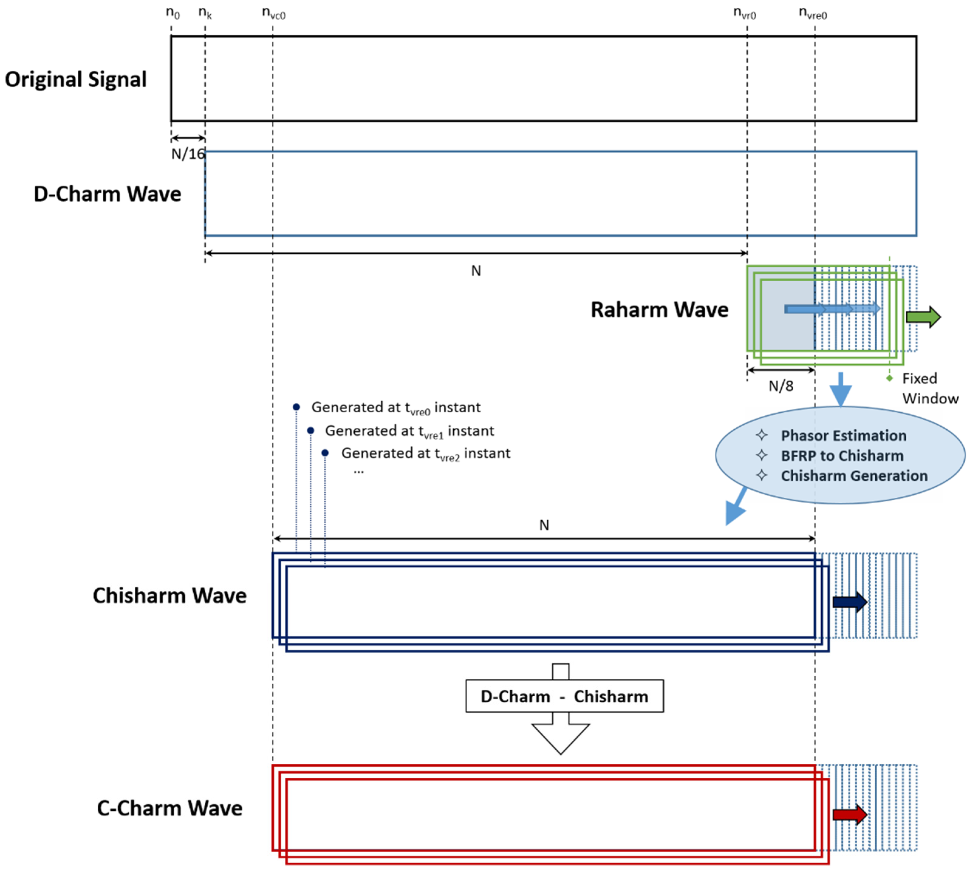
2.2. Obtaining the C-Charm Wave

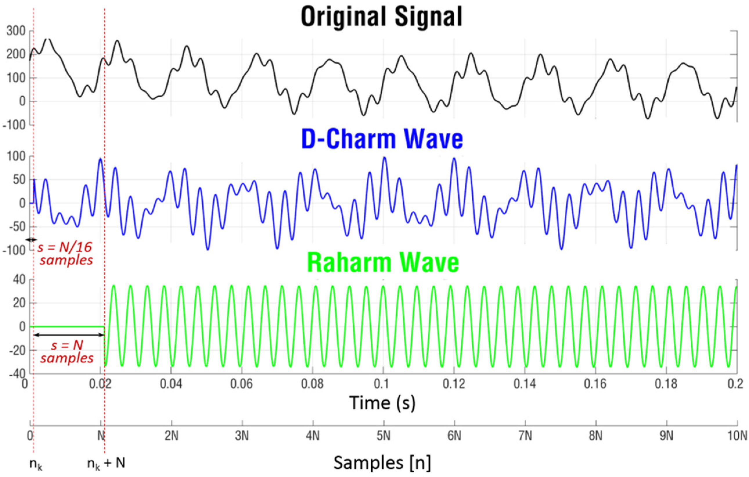
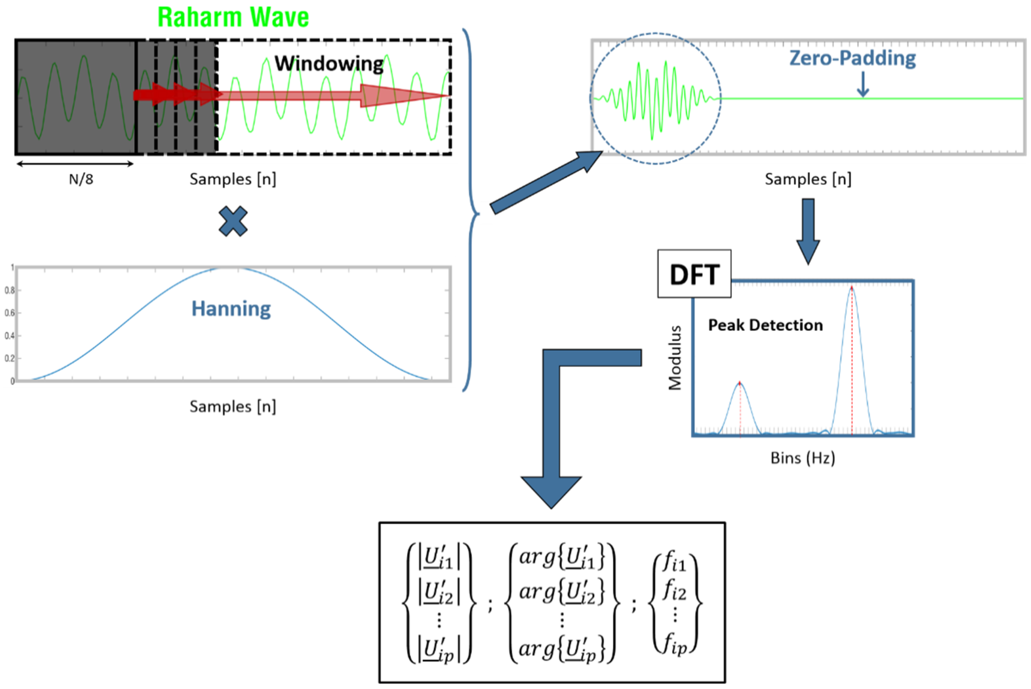
The process of obtaining the C-Charm signal is divided into two fundamental parts. First, starting from the original signal as indicated in (1), the intention is to obtain a signal free from the exponential component. This signal is called the D-Charm Wave (Dirtied Characteristic Harmonic Wave) since it will be a characteristic signal made up of harmonic terms, but it will be “dirty” at the same time because of interharmonic components. To achieve this signal, the STF technique will be applied with the consecutive subtraction of pairs of samples separated from each other by a distance or slip of $s$.

If an approximation is made to the McLaurin Polynomial of the first degree on the term referred to the exponential component in the expression of the original signal (1), for an initial generic $t_0$ instant, the following expression results:

$${ y[n}_0{]=C}_{\mathit{dc}}+C·\left(1-\frac{n_0{T}_s}{\tau }\right)+{\displaystyle \sum }_{h=1}^l{A}_h·\cos \left(2\pi f·h·n_0{T}_s{+\alpha }_h\right){+i[n}_0{]+z[n}_0]$$

(15)

In addition, for a later $t_k$ instant corresponding to a slip of $s$ samples, the resulting expression is:

$${ y[n}_k{]=C}_{\mathit{dc}}+C·\left(1-\frac{n_k{T}_s}{\tau }\right)+{\displaystyle \sum }_{h=1}^l{A}_h·\cos \left(2\pi f·h·n_k{T}_s{+\alpha }_h\right){+i[n}_k{]+z[n}_k]$$

(16)

Subtracting (16) and (15), we obtain the D-Charm signal; for pairs of consecutive samples, this will generally be:

$$\mathit{DCharm}\left[n\right]=-\frac{C·s·T_s}{\tau }+u\left[n\right]+z\prime \left[n\right]$$

(17)

where $u\left[n\right]$ for two samples separated by a number of $s$ samples is the difference between the global contributions of all harmonic and interharmonic components present in the sampled signal, and $z\prime \left[n\right]$ represents the omnipresent white noise in the new signal.

The new D-Charm signal will be composed of a function of harmonic and interharmonic periodic components, noise, and a continuous offset value of $-C·s·T_s/\tau$. The contribution of this offset will be less significant with a slower decay of the exponential, that is, with a higher time constant ($\tau )$, a lower initial value ($C$), and a smaller value taken for the slip ($s$). The value of the sampling frequency ($f_s$) is also important since the less spread out the samples are from each other—equivalent to having a shorter sampling period ($T_s$)—the less influence the term will have.

Given that the $C$ and $\tau$ values of the exponential component are unknown, the only parameters that it can be acted on are the sampling frequency $f_s$ and the slip $s$. The sampling frequency is limited by the DSP used, among other things, in terms of speed and operational calculation capacity between the samples. For this reason, we logically think about the value of the slip $s$ becoming as small as possible.

Although it can be assumed that the most suitable value for the slip may be $s=1$ (two consecutive samples), it must be taken into account that by subtracting samples that are very close to each other, the existing noise in the signal can hide the resulting value of the wave being estimated, distorting its measurement. In this case, the noise can prevail over the value of the signal, or in other words, there is an unfavorable SNR (signal to noise ratio) that will make its phasor estimation difficult.

Therefore, a compromise is necessary between the contributions of the exponential and the noise of the signal when defining the most suitable value for the slip $s$. It has been verified by simulations that a slip value of $s=N/16$ for a value of $N=128$ samples per period of the analyzed signal (modern DSP features used in numeric relays oriented to the field of protections) is admissible from the point of view of an acceptable SNR. Likewise, this value guarantees the good performance of the filter against signals that contain fast exponentials, in addition to producing shorter delays when obtaining the auxiliary signal.

Once we have the D-Charm signal, the second key step is to obtain a signal that only has interharmonic periodic terms of the network fundamental component. Following a process similar to the previous one based on STF with the subtraction of pairs of samples over a slip $s=N$, the Raharm Wave (Removed All Harmonics Wave) signal is created, in which the harmonic components (and also the constant terms) of the D-Charm signal are removed.

The D-Charm signal for a later instant referring to a period $T$ of the fundamental signal, equivalent to $s=N$ samples, is represented by the expression:

$$\mathit{DCharm}[n+N]=-\frac{C·s·T_s}{\tau }+u[n+N]+z\prime [n+N]$$

(18)

By subtracting expression (17) from (18), in addition to canceling the corresponding part to the continuous offset due to the contribution of the exponential component of the original signal, all the periodic components that harmonize with the $T$ period of the fundamental component are eliminated. This means that the new Raharm signal will be:

$$\mathit{Raharm}\left[n\right]=u\prime \left[n\right]+z″ \left[n\right]$$

(19)

where for pairs of samples separated by a period of $N$ samples, $u\prime \left[n\right]$ represents the difference between the global contributions of the interharmonic components present in the D-Charm signal, and $z″ \left[n\right]$ indicates the white noise of the new signal.

Figure 4 shows a graphical representation of the original starting signal, the D-Charm Wave, and the Raharm Wave.

At this point, the objective is to estimate the interharmonic components present in the Raharm signal to generate a new signal that contains the values of its phasors referenced to the D-Charm signal. For this purpose, the BFRP technique is applied to the phasor values that will be estimated from the Raharm signal. The new signal obtained is an inter(sub)harmonic signal characteristic of the original wave or Chisharm Wave (Characteristical Inter/Sub-Harmonic Wave). As explained below, the C-Charm signal that will be achieved is obtained from the difference between the D-Charm and Chisharm signals.

If represented by ${\underset{\_}{U}}_i^{\prime }=\left\{{\underset{\_}{U}}_{i1}^{\prime },{\underset{\_}{U}}_{i2}^{\prime },\dots ,{\underset{\_}{U}}_{ip}^{\prime }\right\}$, each possible phasors contained in the Raharm signal, each phasor will be assigned a module, a phase, and an interharmonic frequency:

$${\underset{\_}{U}}_i^{\prime }=\left\{\begin{array}{c}{\underset{\_}{U}}_{i1}^{\prime }\\ {\underset{\_}{U}}_{i2}^{\prime }\\ ⋮\\ {\underset{\_}{U}}_{ip}^{\prime }\end{array}\right\}\Rightarrow \left\{\begin{array}{c}\left|{\underset{\_}{U}}_{i1}^{\prime }\right|\\ \left|{\underset{\_}{U}}_{i2}^{\prime }\right|\\ ⋮\\ \left|{\underset{\_}{U}}_{ip}^{\prime }\right|\end{array}\right\};\left\{\begin{array}{c}\arg \left\{{\underset{\_}{U}}_{i1}^{\prime }\right\}\\ \arg \left\{{\underset{\_}{U}}_{i2}^{\prime }\right\}\\ ⋮\\ \arg \left\{{\underset{\_}{U}}_{ip}^{\prime }\right\}\end{array}\right\};\left\{\begin{array}{c}{f}_{i1}\\ f_{i2}\\ ⋮\\ f_{ip}\end{array}\right\}$$

(20)

Starting from the frequencies $f_{i1}{,f}_{i2}{,\text{…},f}_{\mathit{ip}}$ of each possible interharmonic component detected and using equation (10), the corresponding BFRP to each phasor referenced to the D-Charm signal can be calculated. Bearing in mind that the value of the slip used to achieve the Raharm signal from the D-Charm is $s=N$, and that the frequency $f$ is assigned the value of system network (50 Hz), equation (10) results:

$${\delta }_i=s·\frac{f\prime }{f}·\frac{360}{N}=N· \frac{f_i}{50}·\frac{360}{N}=7.2·f_i \left(\mathrm{degrees}\right)$$

(21)

As a result, the essential values of $\vartheta$ and $K$ can be obtained from equations (11) and (14). In this way, the relationships pointed out in (12) and (13) can be applied to the phase and modulus values of the Raharm signal phasors. These new values constitute the phasor values ${\underset{\_}{U}}_{i1}=\left\{{\underset{\_}{U}}_{i1},{\underset{\_}{U}}_{i2},\dots ,{\underset{\_}{U}}_{ip}\right\}$ of the Chisharm signal:

$${\underset{\_}{U}}_i=\left\{\begin{array}{c}{\underset{\_}{U}}_{i1}=\left|{\underset{\_}{U}}_{i1}\right| \lfloor \arg \left\{{\underset{\_}{U}}_{i1}\right\}=\left|{\underset{\_}{U}}_{i1}^{\prime }\right|\cdot K_{i1}\lfloor \arg \left\{{\underset{\_}{U}}_{i1}^{\prime }\right\}+{\vartheta }_{i1}\\ {\underset{\_}{U}}_{i2}=\left|{\underset{\_}{U}}_{i2}\right| \lfloor \arg \left\{{\underset{\_}{U}}_{i2}\right\}=\left|{\underset{\_}{U}}_{i2}^{\prime }\right|\cdot K_{i2}\lfloor \arg \left\{{\underset{\_}{U}}_{i2}^{\prime }\right\}+{\vartheta }_{i2}\\ ⋮\\ {\underset{\_}{U}}_{ip}=\left|{\underset{\_}{U}}_{ip}\right| \lfloor \arg \left\{{\underset{\_}{U}}_{ip}\right\}=\left|{\underset{\_}{U}}_{ip}^{\prime }\right|·K_{ip}\lfloor \arg \left\{{\underset{\_}{U}}_{ip}^{\prime }\right\}+{\vartheta }_{ip}\end{array}\right\}$$

(22)

The estimation of the ${\underset{\_}{U}}_i^{\prime }$ phasors, corresponding to the possible interharmonic components the Raharm signal may contain, is carried out by applying a methodology based on the DFT and peak detection technique [36]. This process starts once the Raharm signal begins to be generated and there are enough samples of the signal to detect the highest frequency component. Assuming that the antialiasing filter of the digital relay eliminates frequencies above the eighth harmonic, the highest frequency component that can be found in the signal will correspond to 400 Hz. Therefore, the process, which is represented in Figure 5, is carried out as follows:

• When the Raharm signal reaches $N/8$ data samples, equivalent to the period of a 400 Hz component, the signal is windowed.
• The HZP (Hanning and Zero-Padding) technique is applied to the windowing: the windowed signal is multiplied by a Hanning function in order to smooth the spectral response, and enough zeros are added (zero-padding) to the end of the sequence to increase the spectral resolution [37]. This assures the estimation of the non-harmonic frequency components.
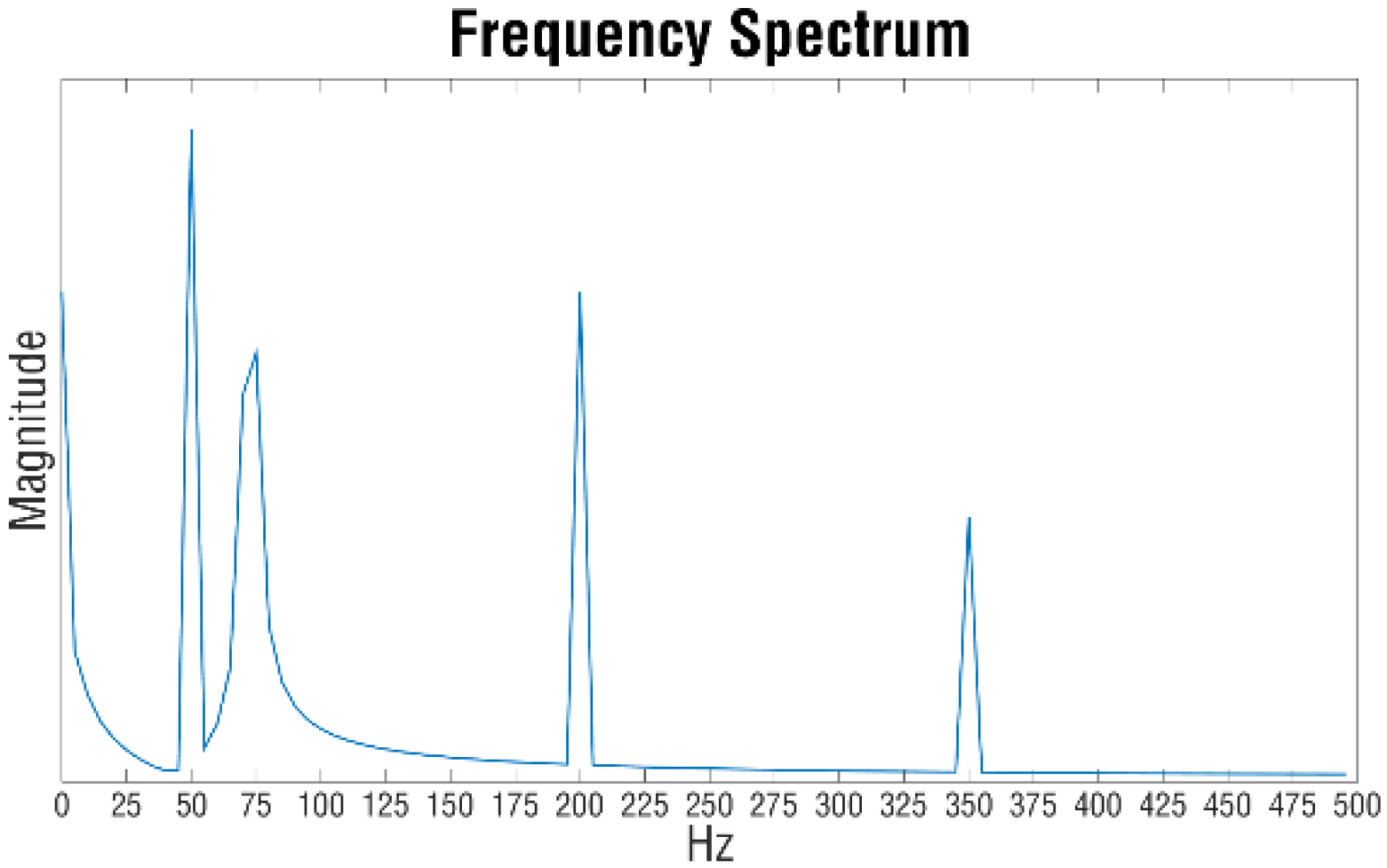
• The DFT is calculated for the previous signal, and the peaks or maximum values are located from the magnitude spectrum. By peak detection, not only can information be extracted from the magnitudes of the components, but the frequency associated with each maximum can also be obtained. Once the frequency is known, the phase of each component can be obtained through the phase spectrum. All the above-mentioned information is easily applicable with a simple programming code and can be verified in the Matlab environment [38].
• For each new sample of the Raham signal, steps 2 and 3 are repeated but with an adaptive data window. The window gains one more Raharm signal sample each time, but one less zero is added. In this way, the increased spectral resolution is maintained.
• The size of the window is set when a certain criterion of values is reached in terms of the magnitude, phase, and frequency of the estimated components. At this point, a suitable window for the correct estimation is considered, and from there, the window advances.
• If the estimated values vary once they have remained constant, this fact will be an indicator that shows that the original signal has changed, and therefore the whole process should be applied from step 1. In this case, it is necessary to re-estimate the new components from the beginning.

As the phasors of the Raharm signal are obtained, the Chisharm signal is created by applying the phasor relationships indicated in (22). The process of creating the Chisharm is carried out on a window of $N$ samples, or fundamental $T$ period, backward from the moment in which the estimation of the interharmonic components begins. In this way, it is possible to obtain signal values of past instants from a current instant. We proceed in this way successively for the subsequent moments. The general expression of the new signal according to the estimated phasors is:

$$\begin{gathered} Chisharm\left[n\right]=\left|{\underset{\_}{U}}_{i1}\right|·\cos \left(2\pi f_{i1}·n{T}_s+\arg \left\{{\underset{\_}{U}}_{i1}\right\}\right)+\left|{\underset{\_}{U}}_{i2}\right|·\cos \left(2\pi f_{i2}·n{T}_s+\arg \left\{{\underset{\_}{U}}_{i2}\right\}\right)+ \\ \dots +\left|{\underset{\_}{U}}_{ip}\right|·\cos \left(2\pi f_{ip}·n{T}_s+\arg \left\{{\underset{\_}{U}}_{ip}\right\}\right) \end{gathered}$$

(23)

Finally, the C-Charm signal (Figure 6), free from both interharmonic and exponential components, is obtained from the difference between the D-Charm signal and the generated Chisharm signal:

$$\mathit{CCharm}\left[n\right]=\mathit{DCharm}\left[n\right] - \mathit{Chisharm}\left[n\right]$$

(24)

For the subtraction to be correct, the lengths of the $N$ samples and the time interval corresponding to the Chisharm window must be taken into account. There is a simplified diagram of the complete process in Figure 7. The D-Charm signal must be consistent with the window corresponding to the indicated samples ${n=n}_{\mathrm{vc}0}$ and ${n=n}_{\mathrm{vre}0}$.

2.3. Phasor Calculation of the Original Signal

Since the C-Charm Wave signal is exclusively composed of harmonic components biunivocally related to the frequency of their corresponding components of the original signal, it is only necessary to estimate their phasors and apply the BFRPs to reference their values to the original ones in the network signal.

Bearing in mind that previous considerations about the antialiasing filter eliminate the highest frequencies of the eighth harmonic, the possible phasors of the C-Charm signal are $U_h=\left\{{\underset{\_}{U}}_1,{\underset{\_}{U}}_2,\dots ,{\underset{\_}{U}}_8\right\}$, where $h$ indicates the order of the harmonic.

Regardless of the moment in which these C-Charm phasors are calculated, the reference that we have with respect to the original signal is a slip of $s=N/16$ samples. Therefore, the expression (10) needed to apply BFRP is:

$${\delta }_h=s·\frac{f\prime }{f}·\frac{360}{N}=\frac{N}{16}· \frac{f_h}{50}·\frac{360}{N}=0.45·f_h \left(\mathrm{degrees}\right)$$

(25)

where $f_h=f · h$ corresponds to the frequencies of the harmonic components, where $f$ is the network fundamental frequency (50 Hz) with $h=1,2,\text{…}8$ due to the cutoff frequency assumed from the eighth harmonic by the antialiasing filter.

In Equations (11) and (14), the values of $\vartheta$ and $K$ are known, which are necessary to apply the BFRPs referred to in (12) and (13) about the C-Charm signal phasors. The ${\underset{\_}{A}}_h$ phasor values of the original signal are obtained thanks to the following relationships:

$${\underset{\_}{A}}_h=| \lfloor {\underset{\_}{A}}_h|\lfloor \arg \left\{{\underset{\_}{A}}_h\right\}=\left|{\underset{\_}{U}}_h\right|·K_h\lfloor \arg \left\{{\underset{\_}{U}}_h\right\}+{\vartheta }_h$$

(26)

The phasors of the original signal are obtained as the phasors of the C-Charm signal are calculated. The windowing of the C-Charm at a window length of $N$ samples, with a period $T$, allows us to apply the one-cycle DFT over the fundamental term without any problems. Thus, both the phasor of the fundamental component and its harmonics are correctly estimated. Once the C-Charm signal is obtained, it is possible to start estimating these phasors of the original signal. As the window advances according to the sampling time ($T_s$), the estimation will continue until there are stable estimated values, which guarantee that the relay protection function is appropriate.

To calculate the interharmonic component phasors present in the original signal, we proceed in the same way as with the harmonic components. If the phasors of the C-Charm signal are used in the case of harmonic components, in the interharmonics case the referenced phasor of the Chisharm signal will be used. Analogous to (25):

$${\delta }_i=s·\frac{f\prime }{f}·\frac{360}{N}=\frac{N}{16}· \frac{f_i}{50}·\frac{360}{N}=0.45·f_i \left(\mathrm{degrees}\right)$$

(27)

where, for $f_i$, we have the possible estimated frequencies indicated in (20).

By means of the BFRP relations, the ${\underset{\_}{A}}_i$ phasor values of the possible interharmonic components of the original signal are obtained:

$${\underset{\_}{A}}_i=\left\{\begin{array}{c}{\underset{\_}{A}}_{i1}=\left|{\underset{\_}{A}}_{i1}\right|\lfloor \arg \left\{{\underset{\_}{A}}_{i1}\right\}=\left|{\underset{\_}{U}}_{i1}\right|·K_{i1}\lfloor \arg \left\{{\underset{\_}{U}}_{i1}\right\}+{\vartheta }_{i1}\\ {\underset{\_}{A}}_{i2}=\left|{\underset{\_}{A}}_{i2}\right|\lfloor \arg \left\{{\underset{\_}{A}}_{i2}\right\}=\left|{\underset{\_}{U}}_{i2}\right|·K_{i2}\lfloor \arg \left\{{\underset{\_}{U}}_{i2}\right\}+{\vartheta }_{i2}\\ ⋮\\ {\underset{\_}{A}}_{iP}=\left|{\underset{\_}{A}}_{iP}\right|\lfloor \arg \left\{{\underset{\_}{A}}_{ip}\right\}=\left|{\underset{\_}{U}}_{ip}\right|·K_{ip}\lfloor \arg \left\{{\underset{\_}{U}}_{ip}\right\}+{\vartheta }_{ip}\end{array}\right\}$$

(28)

3. Results

To show the behavior of the proposed filter, this section presents the results obtained with different types of electrical signals. Two types of signals were defined, and in both cases the sampling frequency used was the same as the modern DSP implemented in protection numerical relays: 6400 Hz for 128 samples/cycle.

• Type A: this type of signal was defined to test the response of the filter to extreme conditions of the analyzed signal. Such conditions can reach more demanding levels than those normally existing in an electrical system.
• Type B: this type of signal was defined to test the response of the filter to situations that originated from faults in an electrical system in transition conditions from pre-fault to post-fault.

In the graphs provided, they are shown for the different cases:

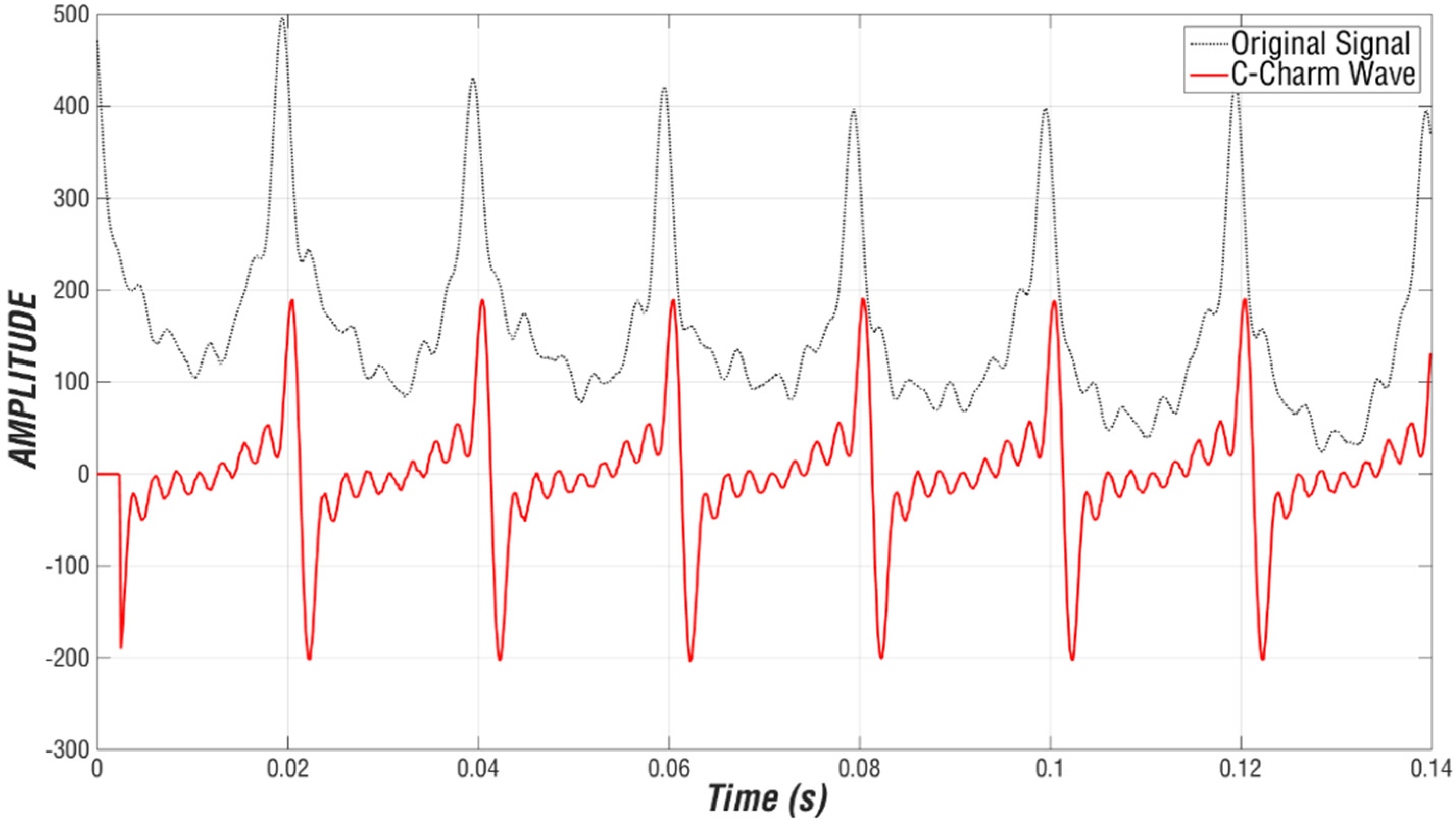
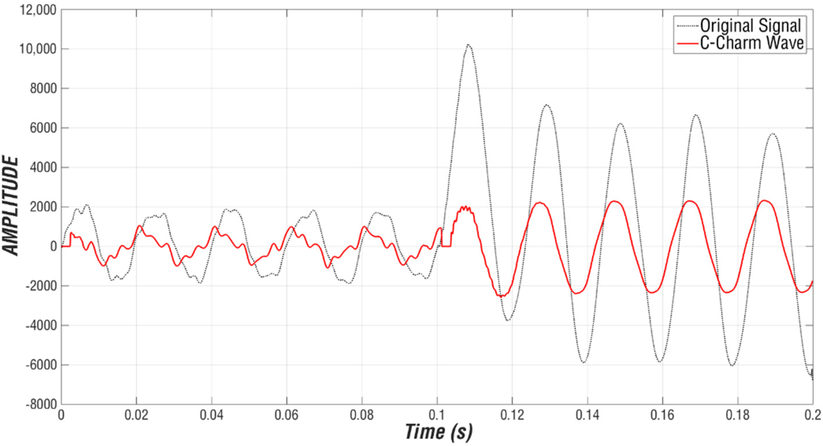
• The original signal and its corresponding C-Charm signal.
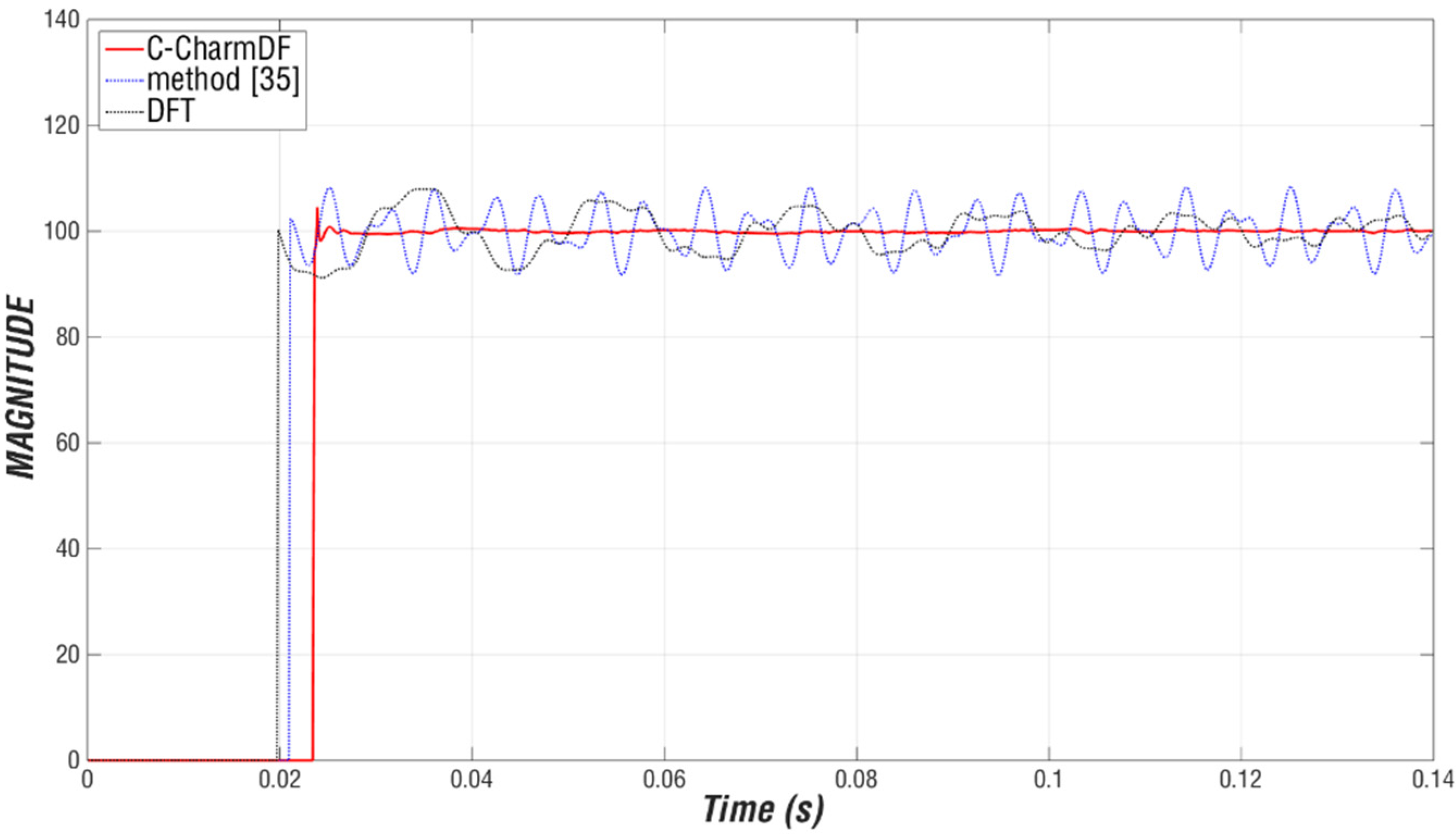
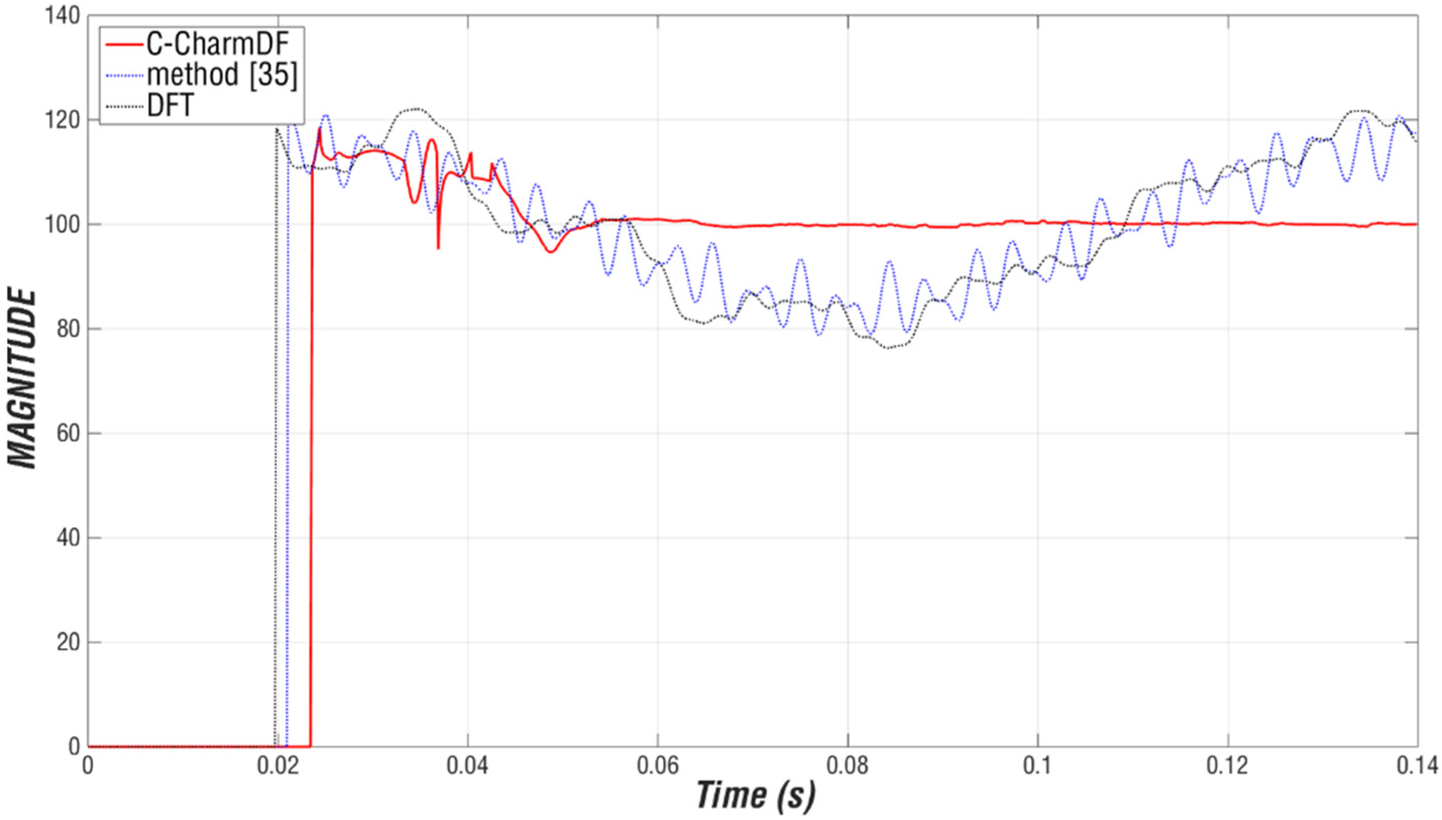
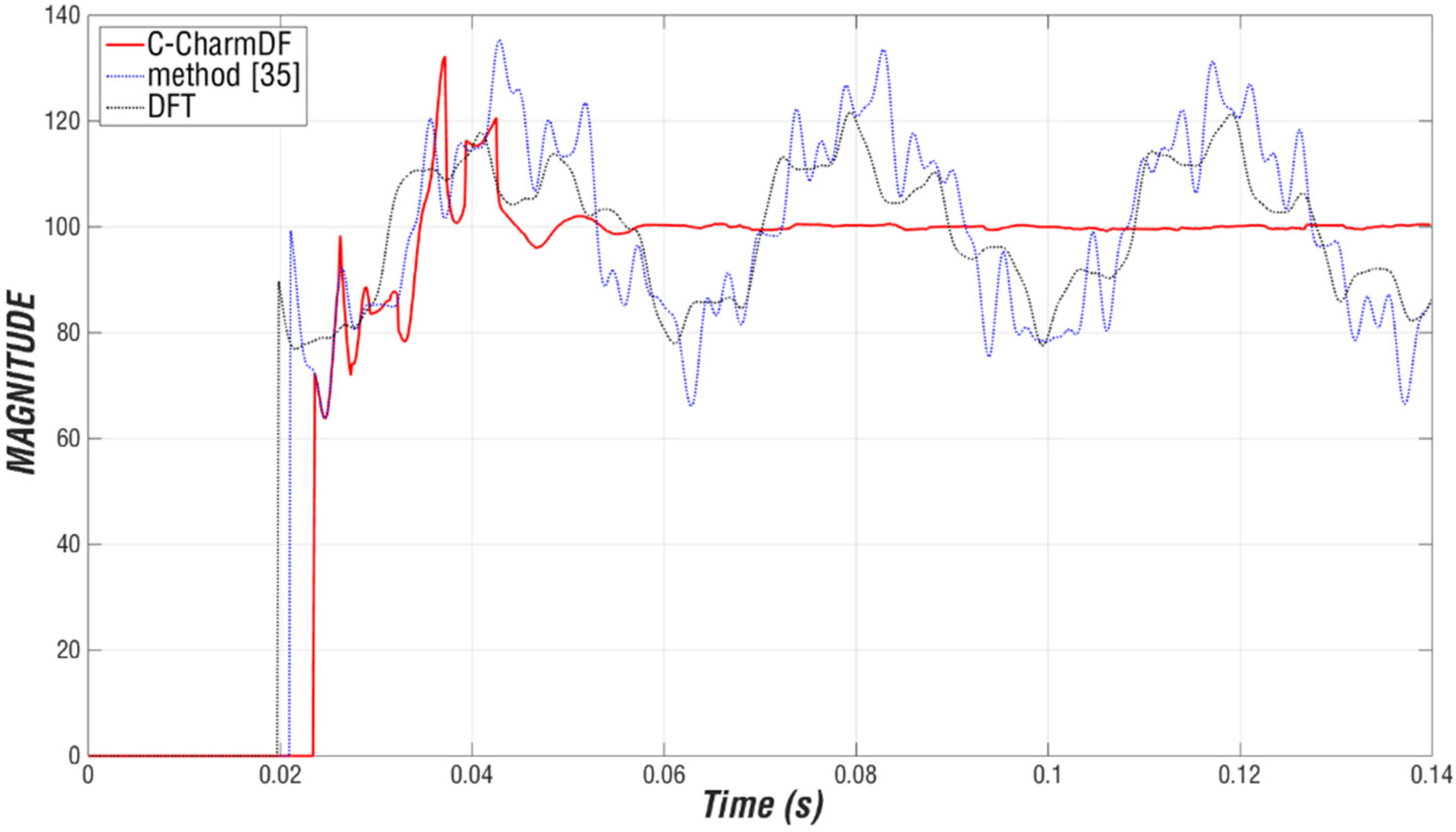
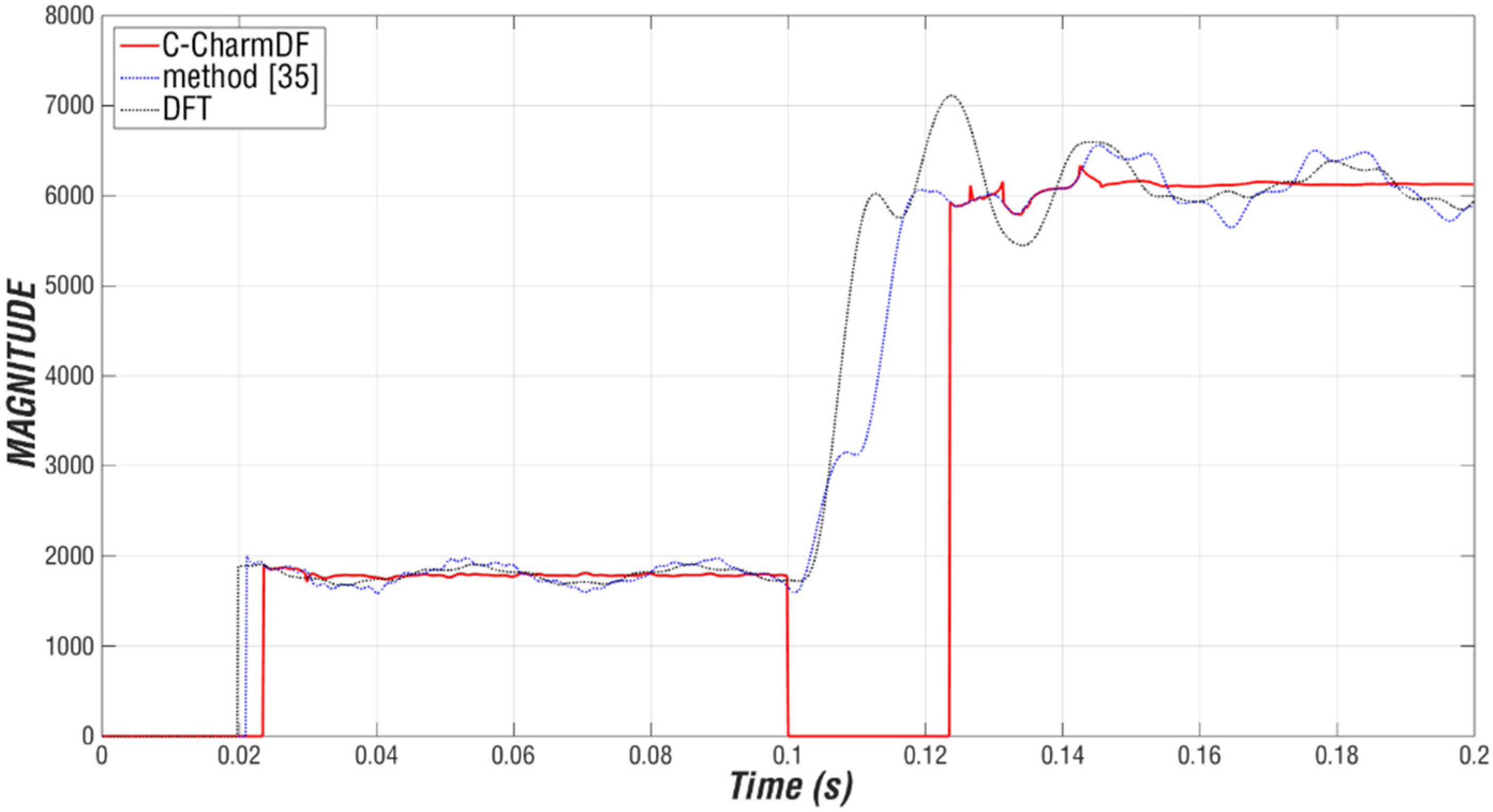
• The estimation of the fundamental phasor modulus, with a comparison of the result applying the DFT and the method proposed in [35].
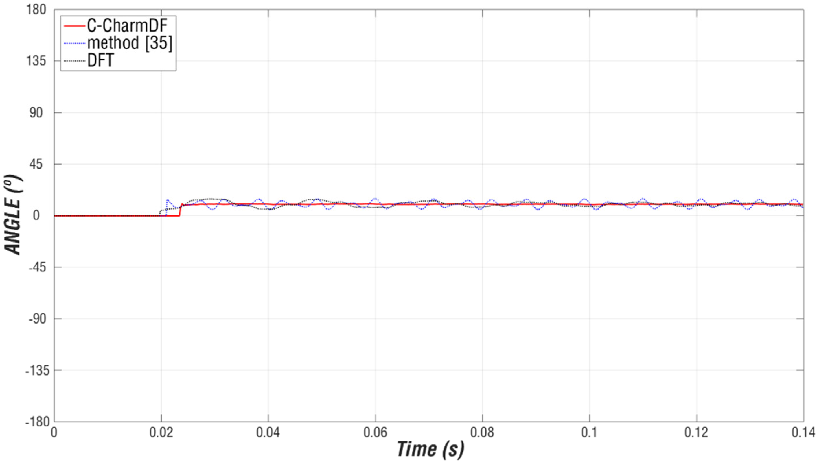
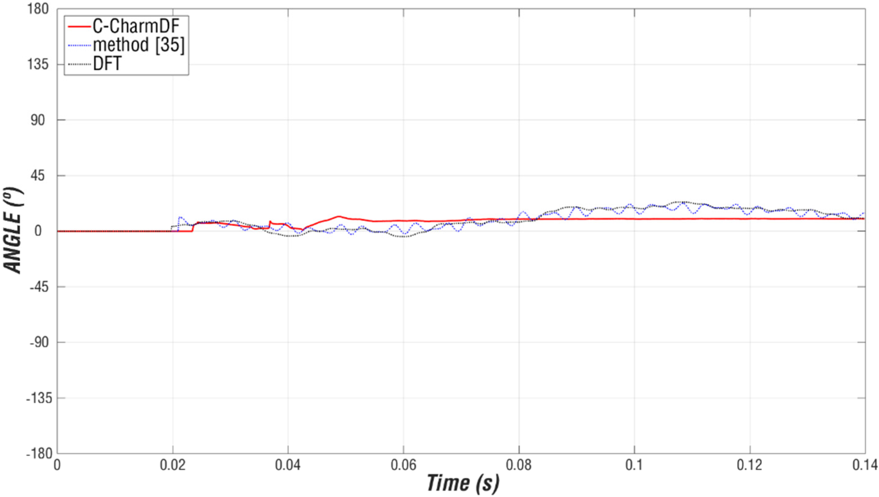
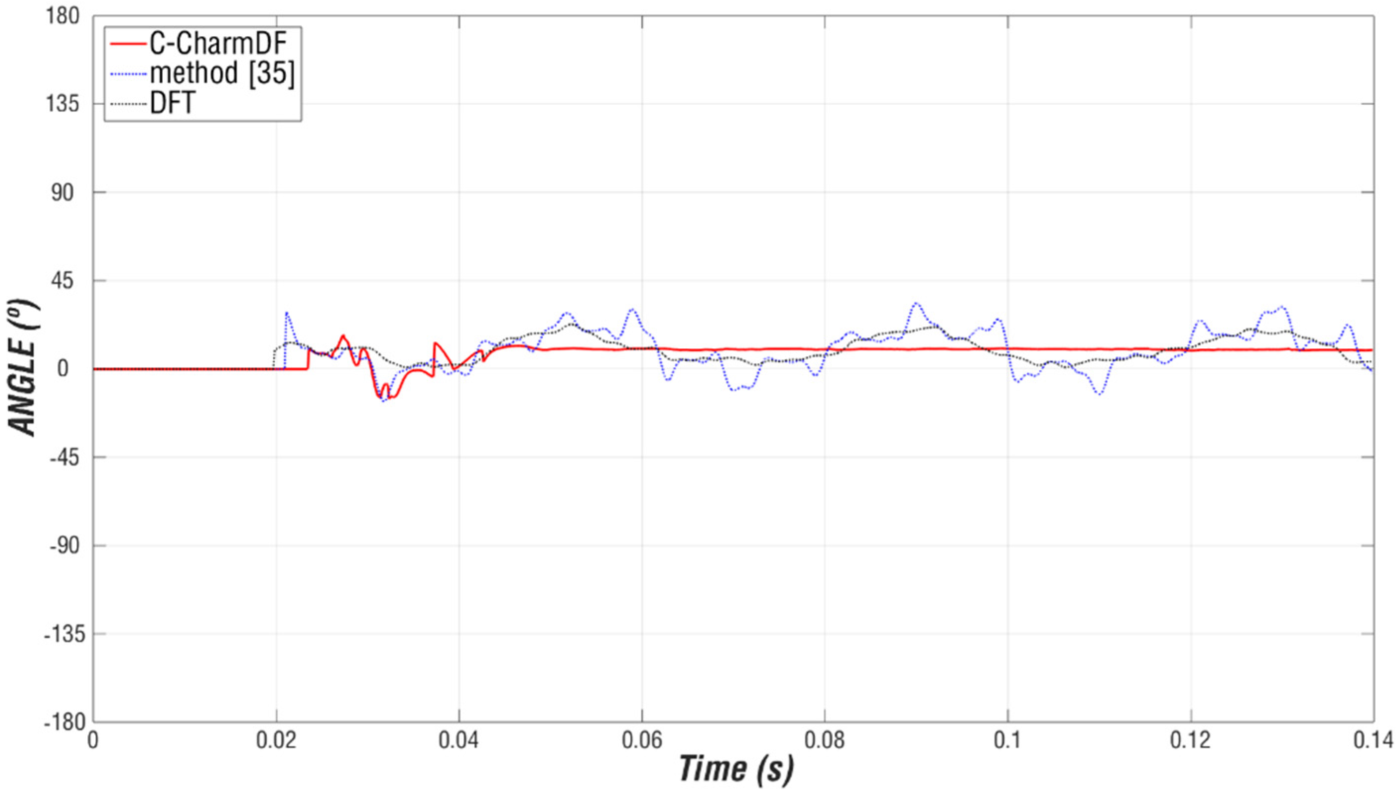
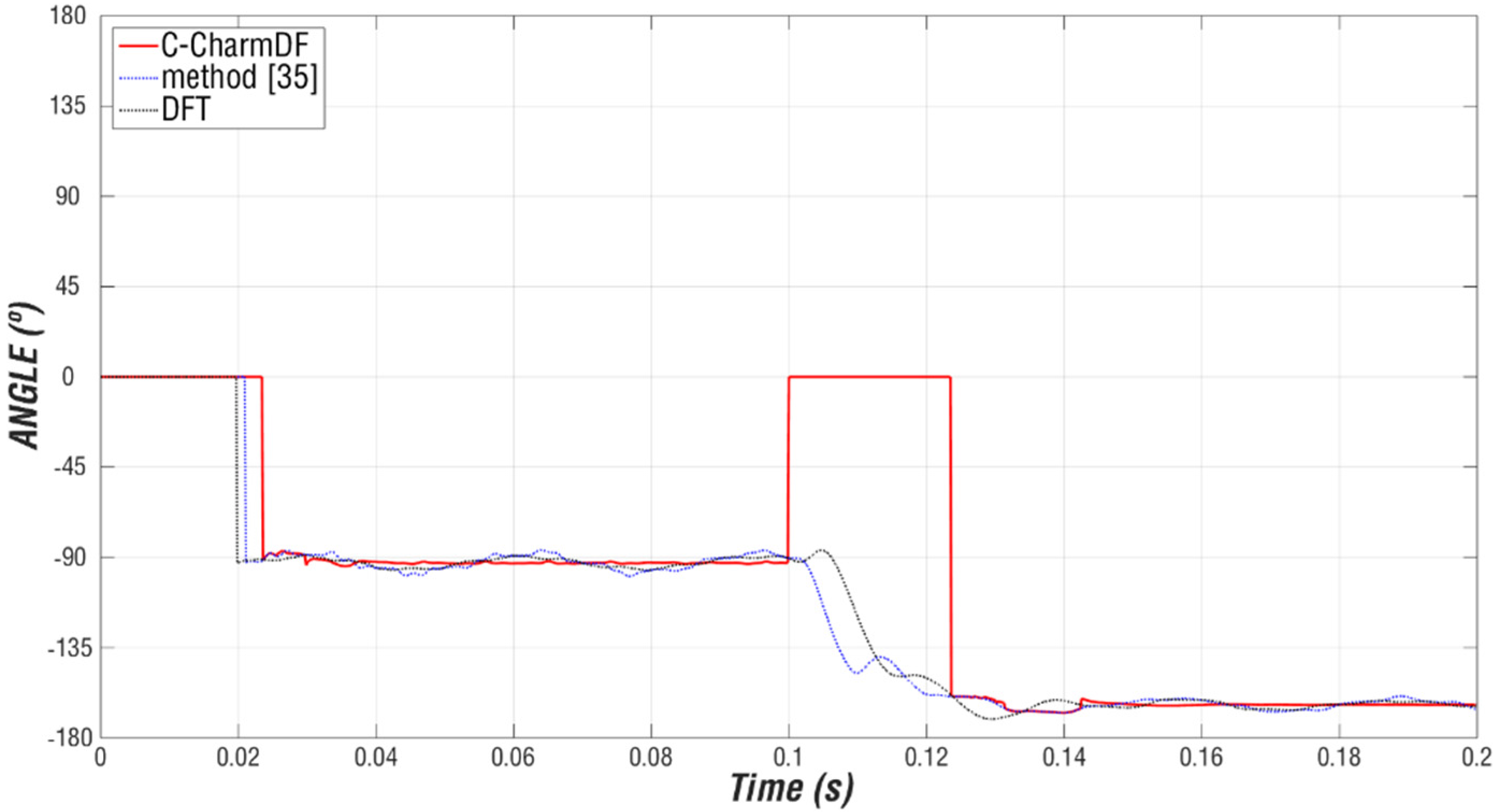
• The estimation of the fundamental phasor angle, with a comparison of the result applying the DFT and the method proposed in [35].

In turn, the IEC 61000-4-30 and 61000-4-7 standards were into consideration in the results obtained [39,40]. These standards contained the measurement methods and interpretation of the results for harmonic and interharmonic distortion. The IEC techniques for the measurement of harmonics and interharmonics established that for the signal observation window, a duration of 10 cycles of the fundamental component of the 50 Hz network is considered, that is, 200 ms. The proposed filter only required a few cycles, at most, for phasor estimation.

Likewise, the interharmonic components detected in the filtering process are indicated for each case in the respective tables.

3.1. Evaluation of the Method for Type A Signals

This type of signal was defined by the expression shown in (1). Three cases are considered with different interharmonic components:

• In Case 1, indicated in

  Table 1. Characteristics of the type A signal for Case 1.

  C0	C1	C2	τ1 (ms)	τ2 (ms)	h	Ah	fh (Hz)	αh (°)	z [n]
  100	80	50	100	50	8	100/h	50h	180h/18	1% A1
  Ai1	fi1 (Hz)	αi1 (°)
  15	230	−40

  , the signal contained an interharmonic component.
• In Case 2, indicated in

  Table 2. Characteristics of the type A signal for Case 2.

  C0	C1	C2	τ1 (ms)	τ2 (ms)	h	Ah	fh (Hz)	αh (°)	z [n]
  100	80	50	100	50	8	100/h	50h	180h/18	1% A1
  Ai1	fi1 (Hz)	αi1 (°)	Ai2	fi2 (Hz)	αi2 (°)
  20	42	30	14	270	−60

  , the signal contained two interharmonic components; one of them subharmonic.
• In Case 3, indicated in

  Table 3. Characteristics of the type A signal for Case 3.

  C0	C1	C2	τ1 (ms)	τ2 (ms)	h	Ah	fh (Hz)	αh (°)	z [n]
  100	80	50	100	50	8	100/h	50h	180h/18	1% A1
  Ai1	fi1 (Hz)	αi1 (°)	Ai2	fi2 (Hz)	αi2 (°)	Ai3	fi3 (Hz)	αi3 (°)
  25	77	45	20	180	−40	15	370	−30

  , the signal contained three interharmonic components.

Assuming that the cutoff frequency of the antialiasing is established in the eighth harmonic, all the harmonic components from the fundamental to the eighth harmonic were considered in all the cases. In each case, the values of the amplitudes of the harmonic and interharmonic components were supposed to be higher than the limits established by the IEEE and IEC standards [41]. At the same time, two decreasing exponential components with considerable values were considered (connected with a real situation of a severe fault that could occur). One exponential may have been caused by the electrical system itself, whereas the other exponential could have been caused by the currenttransformer (by means of which the real signal reaches the protection equipment), for instance, in the case of a currentsignal [27]. Moreover, a continuous DC offset was also taken into account with the same value as the amplitude of the fundamental component and random noise added with maximum levels of 1% of the amplitude of the fundamental component. These conditions provided more demanding extreme signals to the method than those that could be produced in a real system.

The proposed method was applied to estimate the phasor (modulus and angle) of the fundamental component corresponding to each case. The responses obtained throughout the time are shown in different graphs:

• For Case 1, Figure 8 shows the original signal with its corresponding C-Charm Wave and Figure 9 and Figure 10 show, respectively, the estimated modulus and angle.
• For Case 2, Figure 11 shows the original signal with its corresponding C-Charm Wave and Figure 12 and Figure 13 show, respectively, the estimated modulus and angle.
• For Case 3, Figure 14 shows the original signal with its corresponding C-Charm Wave and Figure 15 and Figure 16 show, respectively, the estimated modulus and angle.

It was verified that, in spite of the extreme conditions of the waves used, the following occurred in all cases:

• The response time of the proposed method was independent of the analyzed wave characteristics. According to Figure 7, the response time was the same as ($N/16+N+N/8$) samples (just over one signal cycle) from the moment that the original signal began to be analyzed. This means that the method began to provide results (modulus and angle) just a bit later than one cycle after beginning to receive data.
• The response converged quickly to the correct value (modulus and phase).
• The proposed method reached the solution quickly and, once achieving it, had no significant oscillations, even with severe signals in demanding conditions.
• The other methods were not able to carry out a correct estimation of the analyzed signals.

Thanks to more detailed research, we could determine that:

• The presence of more than one exponential and the added signal noise minimally affected the precision of the proposed method and the speed of its convergence to the correct value.
• The convergence speed depended on the types and numbers of interharmonic components present in the signal. The higher the interharmonic signal frequencies were, the faster and the better the digital filter converged. The slowest interharmonic components in frequency, such as subharmonics, slowed down the convergence process because more signal information was needed to detect them and to make the estimation correctly. Moreover, the increase in the number of interharmonics present in the signal made the process of detection difficult (more noticeable with lower frequencies). This fact meant having higher convergence times to the correct value than those that could be obtained with a lower number of components.

• In Case 1, with a single high-frequency interharmonic, the convergence took place almost immediately from the necessary delay due to processing.
• In Case 2, the convergence was produced approximately one cycle after the processing delay on account of the subharmonic contained in the signal, which delayed the estimation.
• In Case 3, given that the signal contained three interharmonic components, and one of them could be considered slow (frequency close to the fundamental), the method suffered a delay in obtaining the correct phasor values of the fundamental component. This delay was a bit longer than one and a half cycles from the response time.
• In any case, the method converged quickly to the correct value (less than three cycles from the moment that the first information of the analyzed signal was received).

In

Table 4. Detected interharmonic components of the type A signal.

	Ai1	fi1 (Hz)	αi1 (°)	Ai2	fi2 (Hz)	αi2 (°)	Ai3	fi3 (Hz)	αi3 (°)
Case 1	14.98	230	−39.81
Case 2	19.7	41.89	32	14.11	270	−60.69
Case 3	25.1	77.05	43.9	20	180	−39.8	15	370	−29.99

, the results of the interharmonic components detected in the signals in each case are shown. The values are practically identical to the interharmonic phasors of the respective signals.

It was confirmed that the results were sufficiently precise with the sampling frequency used of 6400 Hz, corresponding to 128 samples for a signal cycle of 20 ms (50 Hz). This value is commonly used by the DSP, which the numeric protection relays work with. In any case, it should be pointed out that the proposed method is applicable even though the number of samples per cycle changes.

An increase in the value of the samples per cycle ($N$) would mean an increase, in the same proportion, of the sample frequency ($f_s=1/T_s$) if we want to proceed with a window of one cycle of period $T$ (7). Higher sampling frequencies imply less time to process the data between one sample and the next one. This fact indicates a disadvantage, bearing in mind the current technology for those applications in real-time (or almost real-time). Nevertheless, the following advantages of operating with higher samples per cycle (in case it would be possible) are relevant:

• As explained in Section 2.2, the effect of the exponential term could almost completely be removed by improving the filter response. However, the maximum noise present in the analyzed signal must be taken into account to choose the most suitable s slip value. This requires a compromise between the speed required for the protection and the maximum noise present in the analyzed signal.
• The harmonic and interharmonic components that could be detected could have a higher frequency following the Nyquist theorem [37]. Nevertheless, this is not critical for the method, as the numerical relay antialiasing filter does not allow higher frequencies of 400 Hz (in 50 Hz networks) to go through it.
• The detection of the interharmonic components can be done with higher precision because an increase in the sampling frequency entails a better spectral resolution [36]. Consequently, the phasor detection can be more concrete. This does not imply the possibility of reducing the interharmonics processing and detection time. Having a better spectral resolution does not mean having more spectral information. The interharmonic phasors can be detected with less error but not faster. A higher amount of temporal information is needed for more spectral information. This is the reason why the method uses an adaptive data window of the Raharm signal for the process of interharmonic components estimation.

3.2. Evaluation of the Method for Type B Signals

This type of signal was generated by the Simulink/Matlab Simscape Electrical Toolbox with a verified real network model. This is a signal that includes a steady state (pre-fault) and a transitory state (post-fault). The signal level corresponded to the current signal in one of the phases of a 264 km three-phase line, which had another 78 km three-phase line in parallel and a substation at each of its ends. The fault, between phase and earth, originated within 100 km of the main line. In pre-fault conditions, the signal was composed of the fundamental component (50 Hz) and several harmonic and interharmonic components. These components were randomly assigned, but their values were between the established limits by the IEEE and IEC standards to emulate a real operating situation [41]. In post-fault conditions, in addition to the abovementioned terms, the signal contains decreasing exponential component(s). The program in the context of a fault situation automatically generates all of them.

Figure 17 shows the original signal and its corresponding C-Charm wave. It can be seen that the signal has two situations clearly distinguishable: one pre-fault situation for a normal operating mode of the network and one post-fault situation for a transitory situation of the fault. The results obtained regarding the modulus and the phase for the fundamental component are shown in Figure 18 and Figure 19, respectively. In

Table 5. Detected interharmonic components of the type B signal.

$\mathbf{Pre}-\mathbf{Fault}.$	$\mathbf{Post}-\mathbf{Fault}$
$80 \mathrm{Hz} \mathrm{frequency} \mathrm{component}$	$80 \mathrm{Hz} \mathrm{frequency} \mathrm{component}$
$381 \mathrm{Hz} \mathrm{frequency} \mathrm{component}$	$169.7 \mathrm{Hz} \mathrm{frequency} \mathrm{component}$

, the results of the interharmonic components detected for the pre-fault and post-fault situations are shown.

After analyzing the results, it was confirmed that the proposed method responded correctly to the transition between a stationary state and a transitory one. It was also verified that, as has been highlighted before, the response time of the method was equivalent to just over one cycle once the fault occurred, more precisely, ($N/16+N+N/8$) samples.

In the same way as the type A signals cases, the response converged quickly to the correct value (modulus and phase) and did not present significant oscillations once the solution was achieved. The other methods presented non-convergent oscillations in their results.

4. Conclusions

This article presents a new C-CharmDF digital filtering algorithm for selective estimation of harmonics in noisy fault signals with harmonic and interharmonic components. The method achieved a harmonic characteristic signal, the C-Charm Wave, free of both exponential and interharmonic components, which allowed the phasor estimation process to be carried out with full guarantees. This is thanks to the fact that this wave maintains the necessary information of the periodic harmonic terms of the original signal, thus making it possible to calculate them using the BFRP relationships. In the same way, the used technique guarantees that the effect of noise is minimal, allowing its application even in fault signals with fast transients. The method is also capable of estimating the phasor values of the interharmonic components existing in the signal.

Furthermore, the filter is independent of the instant of fault, thus bringing it closer to the ideal filter. In turn, even with signals composed of interharmonic and subharmonic terms, the phasor estimations converge significantly, avoiding the oscillations of an incorrect estimation. Starting with just over one network signal cycle, the filter was capable of detecting all kinds of periodic components.

In the process of obtaining the C-Charm Wave, the first step is to eliminate the effect of the exponential component(s) present in the original signal. This is achieved by creating the D-Charm Wave using the STF technique from the input signal in question. Starting from the D-Charm and applying the STF technique again, the Raharm Wave is obtained, which is composed only of interharmonic periodic terms. The phasor values of these components are estimated using a DFT-based estimation process (applying windowing and zero padding) and peak detection. Using the BFRP relationships connected with the estimates made, the interharmonic characteristic signal Chisharm Wave is constructed, with which all the interharmonic terms of the D-Charm can be eliminated. By subtracting these two waves properly, the characteristic harmonic C-Charm Wave signal is obtained, free from interharmonic components and decreasing exponential components. Applying the full cycle DFT to the C-Charm, its harmonic components are estimated. The phasor values (modulus and phase) of the original signal are obtained by applying the BFRP relationships on the estimated values, the harmonic phasor values from the C-Charm Wave estimations, and the interharmonic phasor values from those of the Chisharm Wave (referenced from the Raharm Wave).

In addition, the applied methodology is open since it allows the implementation of another series of phasor estimation methods instead of those found in the article, such as container. The phasor estimation methods used can be replaced by others following the same structure (D-Charm, Raharm, Chisharm, and C-Charm processes) and applying BFRP relationships.

The method is valid regardless of the number of samples per cycle used to record the signal. It is confirmed that it is perfectly applicable to the sampling rate currently used by modern DSPs implemented in numerical protection relays. Moreover, the advantages of operating with faster DSPs with more samples per cycle could be beneficial.

A detailed study was carried out on the behavior of the new algorithm to guarantee its stability and precision in the case of noisy signals with interharmonic and/or subharmonic components in both fault and pre-fault states. In the different study cases, it was found that the filter offered superior results to the other methods in the literature. The good work of the filter was confirmed since it required a shorter data acquisition time to carry out its function than that established by the IEC standards, carrying out the estimation process with a minimum margin of error. The above is applicable not only for stationary signals but also for transitory situations that may occur in an EPS.

With an appropriate DSP, all the features provided make the C-CharmDF method suitable for possible application in digital system protection and/or surveillance relays. Regarding fault location applications, the filter requires fewer data. This makes it ideal for application in cases in which only the signal information is available between the instant of the fault and the clearing of it, which is common in fault situations.

The method can be supplementary to the fault detection and classification methodologies. Once the relay has acted, the information of the registered fault signal could be processed in order to obtain the location of the fault almost immediately (in real-time).

The delay in obtaining the phasor response (modulus and phase) is perfectly acceptable, bearing in mind the application field of the present method. There is no doubt that it responds in a more precise and stable manner in comparison with other methods.

References

1. Phadke, A.G.; Thorp, J.S. Computer Relaying for Power Systems, 2nd ed.; John Wiley & Sons: Hoboken, NJ, USA, 2009. [Google Scholar]
2. Pavlatos, C.; Vita, V.; Dimopoulos, A.C.; Ekonomou, L. Transmission lines′ fault detection using syntactic pattern recognition. Energy Syst. 2019, 10, 299–320. [Google Scholar] [CrossRef]
3. Chen, K.; Huang, C.; He, J. Fault detection, classification and location for transmission lines and distribution systems: A review on the methods. High Volt. 2016, 1, 25–33. [Google Scholar] [CrossRef]
4. Pavlatos, C.; Vita, V. Linguistic representation of power system signals. In Electricity Distribution. Energy Systems Series; Springer: Berlin/Heidelberg, Germany, 2016; pp. 285–295. [Google Scholar]
5. Yang, J.Z.; Liu, C.W. A new method for transmission line fault signal phases estimation. In Proceedings of the IEEE ICSS2005 International Conference on Systems & Signals, Kaohsiung, Taiwan, 28–29 April 2005. [Google Scholar]
6. Pan, J.; Vu, K.; Hu, Y. An eficiente compensation algorithm for current transformer saturation effects. IEEE Trans. Power Deliv. 2004, 19, 1623–1628. [Google Scholar] [CrossRef]
7. Sidhu, T.S.; Ghotra, D.S.; Sachdev, M.S. An adaptative distance relay and its performance comparison with a fixed data window distance relay. IEEE Trans. Power Deliv. 2002, 17, 691–697. [Google Scholar] [CrossRef]
8. Rosolowski, E.; Izykowski, J.; Kasztenny, B. A new half-cycle adaptive phasor estimator immune to the decaying DC component for digital protective relaying. Proceedings of Thirty-Second Annual NAPS-2000, Waterloo, ON, Canada, 23–24 October 2000. [Google Scholar]
9. Benmouyal, G. Removal of DC-offset in current waveforms using digital mimic filtering. IEEE Trans. Power Deliv. 1995, 10, 621–630. [Google Scholar] [CrossRef]
10. Gu, J.-C.; Yu, S.-L. Removal of DC offset in current and voltage signals using a novel Fourier filter algorithm. IEEE Trans. Power Deliv. 2000, 15, 73–79. [Google Scholar]
11. Guo, Y.; Kezunovic, M.; Chen, D. Simplified algorithms for removal of the effect of exponentially decaying DC-offset on the Fourier algorithm. IEEE Trans. Power Deliv. 2003, 18, 711–717. [Google Scholar]
12. Sidhu, T.S.; Zhang, X.; Albasri, F.; Sachdev, M.S. Discrete-Fourier-transform-based technique for removal of decaying DC offset from phasor estimates. IET Proc. Gener. Transm. Distrib. 2003, 150, 745–752. [Google Scholar] [CrossRef]
13. Lázaro, J.; Miñambres, J.F.; Zorrozua, M.A. Filtering Techniques: An historical overview and summary of current status. In Proceedings of the International Conference on Renewable Energies and Power Quality (ICREPQ′13), Bilbao, Spain, 22 March 2013. [Google Scholar]
14. Ren, J.; Kezunovic, M. Elimination of DC Offset in Accurate Phasor Estimation Using Recursive Wavelet Transform. In Proceedings of the IEEE Power Energy Society PowerTech, Bucharest, Romania, 28 June–2 July 2009. [Google Scholar]
15. Wong, C.-K.; Leong, I.-T.; Lei, C.-S.; Wu, J.-T.; Han, Y.-D. A novel algorithm for phasor calculation based on wavelet analysis. In Proceedings of the Power Engineering Society Summer Meeting, Vancouver, BC, Canada, 15–19 July2001. [Google Scholar]
16. Liang, F.; Jeyasurya, B. Transmission line distance protection using wavelet transform algorithm. IEEE Trans. Power Deliv. 2004, 19, 545–553. [Google Scholar] [CrossRef]
17. Zahra, F.; Jeyasurya, B.; Quaicoe, J.E. High-speed transmission line relaying using artificial neural networks. Electr. Power Syst. Res. 2000, 53, 173–179. [Google Scholar] [CrossRef]
18. Vasilic, S.; Kezunovic, M. New Design of a Neural Network Algorithm for Detecting and Classifying the Transmission Line Faults. In Proceedings of the IEEE PES Transmission & Distribution Conference, Atlanta, GA, USA, 28 October—2 November 2001. [Google Scholar]
19. Cheong, W.J.; Aggarwal, R.K. Accurate fault location in high voltage transmission systems comprising an improved thyristor controlled series capacitor model using wavelet transforms and neural network. In Proceedings of the Transmission and Distribution Conference and Exhibition 2002—Asia Pacific, Yokohama, Japan, 6–10 October 2002. [Google Scholar]
20. Martinez-Lozano, M.; Martinez, J. Clasificación y Localización de Faltas, utilizando Wavelets y Redes Neurales. In Proceedings of the Noveno Congreso Hispano—Luso de Ingeniería Eléctrica, Marbella, Spain, 30 June–2 July 2005. [Google Scholar]
21. Silva, K.M.; Neves, W.L.A.; Souza, B.A. Distance protection using a novel phasor estimation algorithm based on wavelet transform. In Proceedings of the IEEE Power Engineering Society General Meeting, Pittsburgh, PA, USA, 20–24 July 2008. [Google Scholar]
22. Srivani, S.G.; Vittal, K.P. On line fault detection and an adaptive algorithm to fast distance relaying. In Proceedings of the Joint International Conference on Power System Technology and IEEE Power India Conference 2008 (POWERCON 2008), New Delhi, India, 12–15 October 2008. [Google Scholar]
23. Nam, S.-R.; Park, J.-Y.; Kang, S.-H.; Kezunovic, M. Phasor Estimation in the Presence of DC Offset and CT Saturation. IEEE Trans. Power Deliv. 2009, 24, 1842–1849. [Google Scholar] [CrossRef]
24. Wu, Q.H.; Zhang, J.F.; Zhang, D.J. Ultra-high-speed directional protection of transmission lines using mathematical morphology. IEEE Trans. Power Deliv. 2003, 18, 1127–1133. [Google Scholar] [CrossRef]
25. Buse, J.; Shi, D.Y.; Ji, T.Y.; Wu, Q.H. Decaying DC offset removal operator using mathematical morphology for phasor measurement. In Proceedings of the 2010 IEEE PES Innovative Smart Grid Technologies Conference Europe (ISGT Europe), Gothenburg, Sweden, 11–13 October 2010. [Google Scholar]
26. Byeon, G.; Oh, S.; Jang, G. A New DC Offset Removal Algorithm Using an Iterative Method for Real-Time Simulation. IEEE Trans. Power Deliv. 2011, 26, 2277–2286. [Google Scholar] [CrossRef]
27. Oliveira, A.D.; Silva, L.R.M.; Duque, C.A.; Cerqueira, A.S. Fundamental Component Phasor Estimation in Presence of DC Exponential Decay, Harmonics and Noise. J. Control. Autom. Electr. Syst. 2013, 24, 784–793. [Google Scholar] [CrossRef]
28. Oliveira, N.L.S.; Souza, B.A. Análise da Resposta no Tempo de Algoritmos para Estimação de Fasores utilizados em Relés Digitais. In Proceedings of the IV Simpósio Brasileiro de Sistemas Elétricos (SBSE 2012), Goiânia, Goiás, Brazil, 15–18 May 2012. [Google Scholar]
29. Kim, Y.S.; Kim, C.-H.; Ban, W.-H.; Park, C.-W. A Comparative Study on Frequency Estimation Methods. J. Electr. Eng. Technol. 2013, 8, 70–79. [Google Scholar] [CrossRef]
30. Oliveira, N.L.S.; Souza, B.A. Comparative Analysis of Algorithms for Elimination of Exponentially Decaying DC Component. In Proceedings of the IWSSIP 2012, Vienna, Austria, 11–13 April 2012. [Google Scholar]
31. Miñambres, J.F.; Lázaro, J.; Zorrozua, M.A.; Sánchez, M.; Larrea, B.; Antiza, I. Stability and accuracy of Digital Filters in the presence of Interharmonics. In Proceedings of the 13th Spanish-Portuguese Congress on Electrical Engineering (13CHLIE), Valencia, Spain, 3–5 July 2013. [Google Scholar]
32. Mishra, D.P. Interharmonics Calculation using Adaptive Window Width of time varying load. In Proceedings of the National Conference on Recent Advances in Modern Power Systems (RAMPS-2012), Burla, Odisha, India, 30 December 2012. [Google Scholar]
33. Mojiri, M.; Karimi-Ghartemani, M.; Bakhshai, A. Processing of Harmonics and Interharmonics Using an Adaptive Notch Filter. IEEE Trans. Power Deliv. 2010, 25, 534–542. [Google Scholar] [CrossRef]
34. Zhang, Q.; Liu, H.; Chen, H.; Li, Q.; Zhang, Z. A Precise and Adaptive Algorithm for Interharmonics Measurement Based on Iterative DFT. IEEE Trans. Power Deliv. 2007, 23, 1728–1735. [Google Scholar] [CrossRef]
35. Lázaro, J.; Miñambres, J.F.; Zorrozua, M.A. Selective estimation of harmonic components in noisy electrical signals for protective relaying purposes. IJEPES 2014, 56, 140–146. [Google Scholar] [CrossRef]
36. Dorran, D. Audio Time-Scale Modification. Ph.D. Thesis, Technological University Dublin, Dublin, Ireland, 2006. [Google Scholar]
37. Oppenheim, A.V.; Schafer, R.W. Discrete-Time Signal. Processing, 3rd ed.; Pearson Prentice Hall: Hoboken, NJ, USA, 2012. [Google Scholar]
38. Lyons, R.G. Understanding Digital Signal. Processing, 2nd ed.; Pearson Prentice Hall: Hoboken, NJ, USA, 2004. [Google Scholar]
39. IEC. IEC Std. 61000-4-30. Power Quality Measurement Methods, Testing and Measurements Techniques, 1.0 ed.; IEC: Geneva, Switzerland, 2003. [Google Scholar]
40. IEC. IEC Std. 61000-4-7. General Guide on Harmonics and Interharmonics Measurements, for Power Supply System and Equipment Connected Thereto, 2.0 ed.; IEC: Geneva, Switzerland, 2002. [Google Scholar]
41. Diego García, R.I. Análisis Wavelet Aplicado a la Medida de Armónicos, Interarmónicos y Subarmónicos en Redes de Distribución de Energía Eléctrica. Ph.D. Thesis, Universidad de Cantabria, Santander, Cantabria, Spain, 2006. [Google Scholar]
Figure 1. Frequency magnitudes of a signal with continuous offset, decreasing exponential, and harmonic and interharmonic components.
Energies 14 05166 g001
Figure 2. Process of obtaining the u [ n ] signal from the original x [ n ] signal of f frequency applying the STF.
Energies 14 05166 g002
Figure 3. Phasor diagram of the x [ n ] and u [ n ] signals.
Energies 14 05166 g003
Figure 4. Original signal, D-Charm Wave, and Raharm Wave.
Energies 14 05166 g004
Figure 5. Phasor estimation process of Raharm Wave′s interharmonic components.
Energies 14 05166 g005
Figure 6. C-Charm Wave.
Energies 14 05166 g006
Figure 7. Scheme of the process used to obtain the C-Charm Wave.
Energies 14 05166 g007
Figure 8. Original type A signal and C-Charm signal for Case 1.
Energies 14 05166 g008
Figure 9. Magnitude of the fundamental component of the type A signal for Case 1.
Energies 14 05166 g009
Figure 10. Angle of the fundamental component of the type A signal for Case 1.
Energies 14 05166 g010
Figure 11. Original type A signal and C-Charm signal for Case 2.
Energies 14 05166 g011
Figure 12. Magnitude of the fundamental component of the type A signal for Case 2.
Energies 14 05166 g012
Figure 13. Angle of the fundamental component of the type A signal for Case 2.
Energies 14 05166 g013
Figure 14. Original type A signal and C-Charm signal for Case 3.
Energies 14 05166 g014
Figure 15. Magnitude of the fundamental component of the type A signal for Case 3.
Energies 14 05166 g015
Figure 16. Angle of the fundamental component of the type A signal for Case 3.
Energies 14 05166 g016
Figure 17. Original type B signal and C-Charm signal.
Energies 14 05166 g017
Figure 18. Magnitude in amperes of the fundamental component of the type B signal.
Energies 14 05166 g018
Figure 19. Angle of the fundamental component of the type B signal.
Energies 14 05166 g019