Abstract
The paper presents a study of the critical flow phenomena modeling with MELCOR 2.2.15254 severe accident computer code. The Marviken Critical Flow Test number 21 (CFT-21) experiment was selected as a representative critical flow-focused Separate Effect Test (SET). Various modeling aspects were investigated, including the nodalization, model setup, parameters, and sensitivity coefficients. A local-type sensitivity study was performed to analytically identify the significant parameters and assess their impact on the modeling. A dedicated regression-based approach, using standard deviation, was developed to find the best-fit MELCOR modeling parameters. The primary purpose of this work was to determine the appropriate approach to model critical flow with MELCOR 2.2, investigate the model performance, assess the influence of nodalization choices, identify significant sensitivity parameters, and prepare recommendations with an emphasis on best-estimate modeling. An additional outcome was the benchmark of the recent code version with the Marviken test.
1. Introduction
The MELCOR code is the state-of-the-art severe accident integral computer code developed by Sandia National Laboratories (SNL) and financed by the U.S. Nuclear Regulatory Commission (NRC) [1,2,3]. During the almost four decades of its development, an enormous increase in the understanding of severe accident phenomenology was gained due to extensive experimental programs and developments in modeling [4,5]. At the same time, a substantial increase in the easily accessible computational power occurred, and nowadays, it allows not only to simulate whole accidents in a time scale of hours but also to perform studies for thousands of sensitivity cases. Thanks to these developments, the MELCOR evolved from parametric code with simplified models dedicated to PRA/PSA-2-type studies to the best-estimate code with mechanistic models for most accident-related phenomena [1].
One of the crucial phenomena for Deterministic Safety Analysis (DSA) is the critical flow (choked flow) phenomena [6,7,8,9,10]. Basically, it is a limitation of the flow velocity (flow rate) due to the compressibility of the flowing media for a given pressure difference between the upstream and downstream reservoirs [8]. It occurs during several Design Basis Accidents (DBA) and, especially, for Loss of Coolant Accidents (LOCA) [11]. The thermal-hydraulic system codes like RELAP, TRACE, or CATHARE [12,13,14,15,16,17] are dedicated and able to properly predict this effect, as it plays an important role in the safety assessment, regulatory process, and design of safety systems in nuclear power plants (NPP) [18]. On the contrary, in the severe accident area (and for computer codes like MELCOR), a proper critical flow prediction is typically considered of secondary importance. A long-term mass and energy balance plays the first role for severe accidents with time scales of hours or days, whereas the critical flow has a time scale of seconds [4,5]. Most severe accident tools, including MELCOR, are dedicated to estimating the global progression with a large margin of uncertainty, being larger than for a typical DBA analysis [4,5]. In consequence, the accurate modeling of fast thermal-hydraulic processes, like critical flow, can be treated with less accuracy. Nevertheless, with the growing interest in best-estimate modeling also in the severe accident field, the relative importance of critical flow modeling will likely increase in the future. Moreover, severe accident tools like MELCOR can be used in calculations other than a typical severe accident analysis, including design basis-type studies and regulatory-related research. It can cover studies of the containment performance or dedicated engineering safety features, and accurate modeling of the critical flow can be important [19,20]. This can also be supported by the observation that a severe accident occurs sometime after the appearance of the Postulated Initiating Event (PIE), and it can be necessary to have a computer code that simulates the thermal-hydraulics phenomena occurring prior to the severe accident onset with a proper level of accuracy. The initial course of an accident affects the initial state of the reactor when severe accident phenomena appear, for example, by determining the current value of the decay heat, water levels, or overall state of the plant. Inaccuracies in the initial progression can eventually propagate with accident evolution and amplify the uncertainties [21,22]. The MELCOR code gives the user a lot of freedom in creating a model. It allows both the initial and boundary conditions, as well as the internal parameters of the phenomenological models, to be changed. The user has also plenty of possibilities to develop different model nodalizations. All these factors have an obvious influence on the results. The large flexibility from one point of view is a strength of the tool but also a challenge for less-experienced users. In effect, the flexibility enhances the user effect, magnifying the uncertainties in results.
MELCOR critical flow modeling was discussed and described in the previous paper [23], and its detailed descriptions are available in the Manual [1,2] and are not repeated in this work. The MELCOR code has issues with predicting the critical flow, and they were discussed in previous papers [23,24]. It was earlier discussed by Mosunova in reference [25] and by the code developers in MELCOR Manual [1,2]. The code calculates the subcooled liquid choking flow with the Henry-Fauske model and gas choking flow with reasonable accuracy, comparable to the results achieved by the TRACE code [23,24]. The main problem exists for a critical two-phase flow that is modeled by the Moody model based on the RETRAN code implementation [1,2,3,23]. Future improvements in the MELCOR code will be necessary and are planned by developers [1,2]. However, before these developments, code users have to properly model the critical flow with the currently available code versions and models. Consequently, this work’s primary purpose and motivation were to determine the appropriate approach to model the critical flow with MELCOR. The motivation was to investigate the model performance and prepare the recommendations and best practices with an emphasis on best-estimate modeling. Considering the limitations related to plant scale studies, applying the study results to the NPP simulation will be an ultimate goal. Another purpose was to benchmark the recent code version with the Marviken test and identify which model parameters and nodalization choices impact the results. The previous work focused on the non-code-related parameters, and this work is focused on the MELCOR specific setup and modeling [23]. The additional motivation of this work was to identify the important parameters for future broader global uncertainty and sensitivity analyses focused on critical flow phenomena.
The MELCOR was used to simulate a selected Marviken critical flow test. The Marviken was a Separate Effect Test (SET) large-scale test facility used to carry out numerous experiments. One of them was the Critical Flow Tests (CFT) experimental campaign, which was executed in 1979 and contained 27 tests focused on the critical flow [26]. It was characterized by a low level of scaling with a volume ~400 m3 being close to the volume of the Reactor Coolant System and a relatively high pressure of ~5 MPa. It covered experiments with various nozzle geometries, subcooling conditions, and water levels. The analysis reported in this work is based on the results of test number 21 (CFT-21). The choice was made due to the possibility to compare the results with the validation data based on the validation analysis in the MELCOR 2.1 Assessment report [3]. Test 21 was characterized by a nozzle with a diameter of 500 mm and length of 956 mm, whose Length-to-Diameter (L/D) ratio was 1.9, and it is the value in the middle of the L/D values of the other nozzles used in Marviken (from 0.8 to 4.3). The CFT-21 test is characterized by water being initially subcooled to 33.7 °C, the pressure of 4.94 MPa, and a high water level equal to 19.95 m.
This paper is organized in the following way. Section 1 introduces the topic, motivation, and scope of the paper. Section 2 presents the applied methodology, developed models, approach to perform a local sensitivity analysis, and method to evaluate the best-estimate parameters. Section 3 presents the results of the analysis and discussion, and Section 4 contains the conclusions. All simulations in this work were performed with 2019 MELCOR version 2.2.15254 [1,2].
2. Methodology
2.1. Marviken MELCOR Models
A nodalization preparation is a principal aspect for MELCOR thermal-hydraulics modeling with the Control Volume Hydrodynamics package (CVH) and Flow path package (FL or FP). Typical nodding schemes are coarser than in thermal-hydraulic system codes, contributing to the user effect. Due to that, an effort was made to investigate different nodding approaches. Overall, fourteen different nodalizations of Marviken CFT-21 were prepared (see Figure 1 and Table 1). The choice of nodalizations was motivated by the practices commonly used by MELCOR users when creating computational models. The selected models were primarily intended to represent the most straightforward approach, ensuring short computation times and good computation stability and applicability for the plant scale studies. The models studied in this work were created from scratch and independently from the MELCOR models developed and discussed in previous papers [23,24]. One of the differences compared to previous models is a detailed height–volume table for all the applied control volumes (see Figure 1).
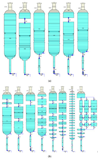
Figure 1.
Marviken MELCOR nodalizations: (a) basic models and (b) complex models.

Table 1.
List of the models used in the simulations with the geometry data and initial conditions. See also Figure 1. The values in the cells present information about their volume, saturation condition, and temperature.
In total, fourteen nodalizations were used in the calculations (Figure 1). The basic nodalization (designation 01A, Figure 1) was selected to represent the simplest and commonly used approach to model the vessels—one control volume for the CVH package with a single flow path (FL package) for a nozzle. On the contrary, the most complex nodalization (designated 24A) contained 24 control volumes. It was selected based on the validation test described in the MELCOR 2.1 assessment report [3], where 21 CVs were applied. The validation results and available experimental data [24] are references for the calculations presented in this work. The densest nodalization provides results considered to be the most accurate in relation to the experiment. However, in practice, it is not practical or not possible to apply it in the case of the modeling of NPP with MELCOR. The reason is the limited computational capabilities of the MELCOR code, e.g., arising from the CFL limit or potential problems with the numerical convergence and stability. It is especially the case when neighboring CVs have significantly different volumes. In order to investigate these issues, it was decided to introduce and study intermediate models.
The first modification of the simplest nodalization was the separation of a CV modeling of the nozzle (02C, see Figure 1). The purpose of selecting this option was to observe the possible computational problems related to the use of interconnected control volumes with significantly different volumes and dimensions in the model. An alternative approach was the separation of one CV to model the nozzle together with the discharge pipe connected to the tank (02B). The next alternative was the division of the upper part of the tank, being in a saturated state (model 02A). This choice aimed to obtain a more detailed nodalization, separating the upper volume of the vessel with water in the saturated state. Two additional nodalizations with three CVs were developed—03A and 03B. 03A combines 02A and 02B—it includes the separate volume for saturated water and has a separated nozzle CV. On the other hand, model 03B is a variant of 02C with a separate nozzle control volume. Moreover, three models with four CVs were developed and denoted as 04A, 04B, and 04C. Nodalization 04A is a variant of the 03A with additional volume for the interface of saturated water with subcooled water. Model 04B is based on 02B but with the vessel divided into three CVs with similar volumes. Finally, the nodalization 04C is a variant of 03A with an additional volume for the nozzle.
The next approach used to determine the nodalization was to ensure that the subsequent CVs linked with flow paths have volumes differing from each other no more than two times. It is a more-or-less arbitrary limit based on the engineering experience with system codes. As a result of the applied principle, the 08A nodalization was created, consisting of eight control volumes (see Figure 1). The purpose of this approach was to observe the differences in the results between the nodalizations of different spatial densities. In order to determine the 06A model, the main vessel was divided into CVs having almost the same volumes—similarly to 04B. Thanks to this, it was possible to compare the 06A and 08A nodalizations with a similar nodding density but a different approach to determine the individual CVs.
Afterwards, the 08A model was modified by adding a separate CV for the nozzle (09A). The extracted volume did not meet the two-times-smaller volume requirement, as it was 11.6 times smaller than the adjacent volume. The purpose of creating this nodalization was to compare similar models differing only by the isolation of an additional small control volume for the nozzle.
The next nodalization (designated 3 × 3) was based on the approach recommended by the developers of the MELCOR code for modeling the control volumes of the reactor pressure vessel (RPV). Clearly, it is not the same modeling problem, but the approach may be similar. The Marviken vessel, with a net volume of about 424 m3 and an internal diameter of about 5.2 m, has comparable geometry to an RPV of a typical PWR with a net volume of about 100 m3 and an internal diameter of about 4.0 m. The CFT test has a one-dimensional nature, and higher dimensional effects are relatively unlikely to occur or eventually unlikely to produce observable effects. However, in order to confirm this hypothesis, the model was prepared, and it was tested in this work. The model with three rings and three axial levels was prepared. In addition, one CV at the top of the tank was extracted, similar to RPV Upper Head modeling. The lower part of the tank was divided into three levels, similar to Lower Head modeling in the RPV. The discharge pipe, together with the nozzle, was modeled with a separate control volume. Altogether, this nodalization significantly differs from the others by introducing horizontal flow paths between the control volumes and allowing the medium to cross-flow and eventually flow upwards and downwards simultaneously in the tank during the simulation.
2.2. Initial and Boundary Conditions
The issue that arose when creating different nodalizations was the temperature averaging procedure in the control volumes. The averaging was made based on the experimental data [26] and using the information on the net volume at individual levels of the vessel. It was assumed that the temperature measurement carried out during the experiment at a given level of the tank is an average value in the volume from half of the distance between the given measurement and the adjacent measurements. In order to determine the mean temperature of a given control volume, Equation (1) was applied.
where n is the number of volumes, i is the index, and ΔV is incremental volume. It is the mean temperature weighted with the volume.
The initial conditions, including the temperature, pressure, and water level, were taken from the experimental data [26]. The temperatures and geometry details for the CVs for each nodalizations are described in Table 1.
An important issue in determining the boundary conditions is selecting the values of the parameters describing the flow paths between individual control volumes. In order to eliminate the influence of the flow path settings on the performed local sensitivity analyzes, it was decided that each model would have as similar a flow resistance as possible. For this purpose, when describing the individual flow paths for a given model, care was taken to ensure that the sum of the lengths of individual segments for all thr flow paths for a given model is identical to the values determined for the simplest 01A nodalization. The value of the local flow resistance was estimated analytically based on the physical design of the experimental installation. Each of the nodalizations takes into account these local flow resistances so that the sum of local flow resistances for all the paths making up a given nodalization is the constant value that is the same for all the models.
In the case of 3 × 3 nodalization, it was necessary to determine the parameters of the horizontal flow paths. For this nodalization, it was also necessary to divide one flow path into three flow paths assigned to each of the rings. The use of this nodalization forced the change of the surface area values for these flow paths in relation to the values assigned to the other nodalizations. The impact of changing the hydraulic diameters for the flow paths covered by this issue was analyzed (flow paths 141–143, 151–153, and 161–163—see Figure 1b), and the impact was negligible; therefore, it was decided that, for these parallel flow paths, the hydraulic diameter would remain unchanged.
2.3. Sensitivity Parameters
The initial conditions, including, e.g., the initial vessel pressure, temperature, water level, and initial pressure in the containment, were eliminated from the sensitivity analysis. It was also the case for the boundary conditions, definitions of the geometry (e.g., cross-sectional area, length and hydraulic diameter for individual segments of the flow path/paths, pipeline roughness, total length, and surface area of the flow path).
The initial analysis covered the systematic study of the extended list of the parameters available in the MELCOR code, which were identified to have a potential impact on the thermal-hydraulics and critical flow results. These parameters are presented in Table 2 and are shortly discussed below. The set of parameters covered the following sensitivity coefficients and parameters: discharge coefficients (FL_USD card), momentum exchange length (FL_LME), and momentum flux areas (FL_MFX) for the flow paths in the model, heat, and mass transfer coefficients for the pool and atmosphere (SC4407) in the control volumes, flashing model parameters (SC4500), and minimum velocity for the choked flow (SC4402). An analysis was performed for the three selected models: 24A, 06A, and 02A. This step was performed to preselect the parameters to be studied with all the nodalizations in the next step. In order to thoroughly investigate the influence of the parameters, wide ranges of values were assumed for the initial analysis.
Table 2.
List of the sensitivity parameters studied in the initial analysis. The parameters were available in the code version 2.2.15254 and taken from the Manual [1,2].
The initial analysis performed for models 24A, 06A, and 02A showed that most of the parameters presented in Table 2 do not significantly influence the Marviken critical flow test modeling outcomes. In all of these cases, the change in standard deviation (described in Equation (2)) of the obtained results was below 3%, but for many cases, it was well below 1%. In consequence, the reduced number of parameters was used to study all the other nodalizations. The variability range was reduced to limit the outcomes to be more physically reasonable. The list of parameters selected for the further part of the study is presented in Table 3.
Table 3.
List of the sensitivity parameters selected for the final analysis.
During the initial analysis, when modifying the MELCOR card related to the momentum flux flow area in a flow path (FL_MFX, item 3 in Table 2), it was observed that it impacted the results for the model with fine nodalizations. On the contrary, for the coarse models, there was no impact. Nevertheless, it was decided to omit this parameter in the further analysis and use the value of the physical area as a more reasonable choice.
For all the selected nodalizations, local sensitivity analyzes were carried out to obtain the best-fit results. The best-fit results are calculations performed for the reference model with the best-fit parameter. The values of the individual parameters for individual nodalizations that allow obtaining the best fit with the experiment results are presented in Table 3 and discussed in Section 3. The base case default models in this work are models using the default MELCOR values for almost all the parameters. The exception was the sensitivity coefficient (SC4402(1)) defining the minimum velocity considered in the choking calculations, and it was set to 0.0001. It was observed that this coefficient is at least partially responsible for the numerical oscillations for the subsequent time steps. However, it is more important for larger values, and the selected value is very low. This approach is more a conservative “safety” measure to rule out possible problems during the calculations, with a relatively low price in computational time. The code default value is 20.0 m/s, and for values below 25 m/s, problems were rarely observed. Effectively, the results obtained with low values are equivalent to the results obtained with the code’s default value.
2.4. Regression-Based Best-Fit Approach
In order to evaluate the results obtained for individual runs, the value of the standard deviation-like parameter was used, as defined by Equation (2). Later in the text, this parameter is referred to as the standard deviation. This approach allows changing the vector value of the break flow in time into a scalar value, simultaneously determining the degree of compliance of the obtained results with the experimental data. This approach was inspired by machine learning methods for a regression analysis [27]. It simplifies the analysis of the obtained results and facilitates their evaluation. It is also an approach that allows comparing two datasets with a different number of time-dependent values in a given interval.
where n is an arbitrarily selected number of time intervals for the time interval equal to 60 s, being the experiment duration (adopted n = 20), i is an index of an interval, xi is an average value for a figure of merit in the time interval i, and Yi is an average value for the experimental data in the time interval i.
3. Results and Discussion
3.1. Results for Default MELCOR 2.2 Settings
In this subsection, the results for all fourteen base case models with the default MELCOR setup are presented and compared—see Figure 2, Figure 3, Figure 4, Figure 5 and Figure 6. The results are also compared with the experimental data and MELCOR reference results for the 21CV and 1CVs (see Figure 2 and Figure 7). The presented results are the basis for the further sensitivity studies in Section 3.2.
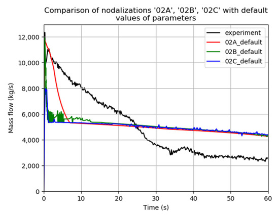
Figure 2.
Mass flow rate for the models with 2 CV 02A, 02B, and 02C nodalizations compared with the experimental data.
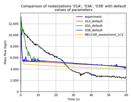
Figure 3.
Mass flow rate for the models with 1 CV and 3 CV 01A, 03A, and 03B nodalizations compared with the experimental data and MELCOR results taken from reference [12].
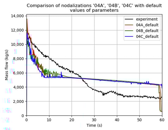
Figure 4.
Mass flow rate for the models with 4 CV 04A, 04B, and 04C nodalizations compared with the experimental data.
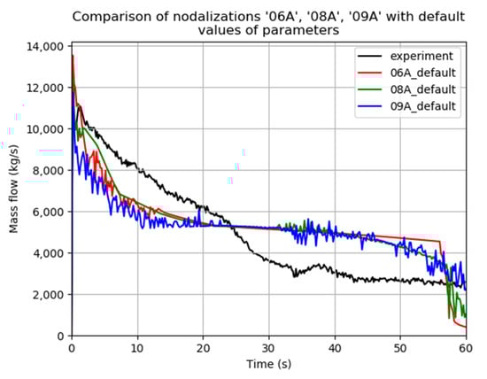
Figure 5.
Mass flow rate for the models with 6, 8, and 9 CV 06A, 08A, and 09A nodalizations compared with the experimental data.
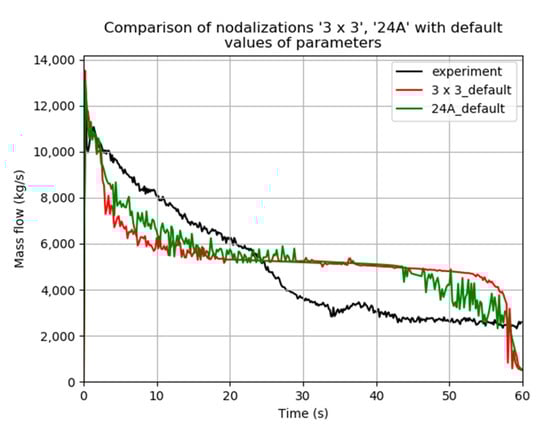
Figure 6.
Mass flow rate for the 3 × 3, 24A nodalizations compared with the experimental data.
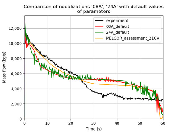
Figure 7.
Mass flow rate for the 08A and 24A nodalizations compared with the experimental data and MELCOR results taken from reference [3].
It is worth noting that the presented results were not smoothed or altered in any way. Therefore, the results are “raw”, so one can clearly observe the influence of the selected nodalization schemes. For several cases, the oscillations can be observed, which likely have a numerical origin. The considerable variations of the selected models give the opportunity to assess the influence of nodalization and, eventually, identify the source of the oscillations.
In all fourteen calculations, MELCOR underpredicted the length of the initial subcooled flashing phase of the critical flow and subsequently overestimated the two-phase critical flow part of the test (see Table 4). The duration of the critical flow during a LOCA accident (tens or hundreds of seconds) is incomparably shorter than the time after which a severe accident may occur (several hours). From the safety analysis point of view, overestimation of the two-phase flow allows for obtaining more conservative results and a faster emptying of the reactor cooling system than in reality. This overestimation results from the Moody model, which overpredicts the two-phase flow rates for steam qualities larger than 1%. This model causes the rapid formation of high steam concentrations in pipes [28]. Therefore, the results obtained using the MELCOR code can be considered acceptable for some applications, but the reader has to be aware of these issues. Nevertheless, the total integrated mass flow at the end of the test is comparable between the experiments and calculations regardless of the selected nodalization. It is worth observing that the switch between the flashing flow and two-phase flow in the MELCOR code depended on the number of control volumes. The flashing phase was the shortest for the model with one node (Figure 3 and Table 4), while the most extended flashing phase was observed for the nodalizations with more than four control volumes (Figure 5 and Figure 6).
Table 4.
Standard deviations for the default calculations using different nodalizations. Experimental maximum flow of 12,347 kg/s. Experimental time of the flashing flow of ~30 s.
Using the standard deviation defined in Equation (2) as a measure to assess the ability of a model to reproduce experimental data, it was determined which nodalizations allowed to obtain the best-fit results being most similar to the experimental data. The standard deviations for each case are presented in Table 4, along with the values of the maximal mass flow for each case. The best results were obtained using models 24A and 08A. The value of the maximum flow in the experiment was 12,347 kg/s. The maximum flow values (from 10,319 to 13,567 kg/s) obtained for most of the nodalizations were consistent with the experiment results. On the contrary, the 02C nodalization stands out, as its maximum flow is significantly underestimated and has a value of 7987 kg/s.
Figure 2 and Figure 3 represent the results for nodalizations with one, two, or three control volumes. The outcomes for cases 01A, 02B, 02C, and 03B are very similar, albeit with oscillations present in the cases of the 02B and 03B nodalizations. Comparing the obtained results with the SNL results for one CV (Figure 3 yellow line), a good agreement can be found. In the case of nodalizations 02A and 03A, one may observe that the flashing phase lasts longer; therefore, the results for those models provide a slightly better representation of the observed phenomena. The vessel was split into two parts for these two models, one with saturated and one with subcooled conditions. Nodalization 03A is also characterized by the presence of a discharge pipe as a separate control volume. The division of the discharge pipe is probably responsible for the oscillations that may be observed in the subcooled flashing phase (Figure 2). Models 02B, 02C, and 03B introduced separated single control volumes for the discharge pipe and/or nozzle. This approach leads only to the presence of more oscillations and a shorter time of the flashing phase. For nodalization 02C, one may also observe that the maximal mass flow is the lowest of all the analyzed cases; therefore, a model with one control volume for the vessel and one for the nozzle provides the worst prediction. As indicated by Table 4, those were the nodalizations (along with 01A) characterized by the highest values of the standard deviation with respect to the experimental results. It can be observed that the separation of the sub-cooled and saturated region changes the time scale of the flashing period quite significantly, as shown for models 02A and 03A and other, more complex models.
Figure 4 presents the results for the nodalizations with four control volumes. One can observe that the flashing phase lasted longer than for the nodalizations with less than four nodes. The results for 04A, 04B, and 04C are relatively similar, but one can observe that, for the 04B model, the flashing phase ends about 9 s later than in the 04C model. Differently, model 04A predicts a larger maximum mass flow ~13,500 kg/s, and for 04C with CVs for the nozzle, it is about ~2000 kg/s lower. All three cases are characterized by the presence of oscillations in the subcooled flashing phase.
Figure 5 presents the results of the calculations for the nodalizations with six, eight, and nine control volumes. The introduction of more nodes increased the length of the flashing phase, as observed previously. For 06A and 08A, it is about 20 s, and for 09A, it is slightly less. The results for the nodalization of 08A are characterized by a lack of oscillations in the flashing phase and closest fit to the experimental results, especially during the first 5 s. The standard deviation with respect to the experimental results (see Table 4) is low, and only 24A has a lower value. Once again, adding separate control volume for the nozzle (nodalization 09A) resulted only in the appearance of oscillations without an improvement of the results. Based on the results of the model of 09A, it can be concluded that the introduction of a small volume in the nozzle region is a likely significant source of observed oscillations. Similarly, based on the results for the nodalization of 08A, it can be concluded that the second source of oscillations is due to the presence of small volumes (also for 09A) at the bottom of the vessel, as these are not present in 06A.
Figure 6 presents the results for the two most complex nodalizations 3 × 3 and 24A. The 3 × 3 case does not present an improvement in comparison to the nodalization of 08A (see Figure 5). Oscillations were observed in the flashing region; therefore, this nodalization can be deemed inferior with respect to the nodalization of 08A. The results for model 24A may be assessed as the best in comparison to all the studied cases, as expected from the beginning. The difference between the experimental data and the calculation results of 24A is the lowest (as indicated by the standard deviation, introduced in Table 4). Although those results are also characterized by the highest oscillations (together with 09A).
Figure 7 shows a comparison of the results obtained with the 08A and 24A models, which were considered the best, compared with the validation SNL results (yellow line) and experimental data. The results obtained in this work are similar to the SNL results, with a slight underestimation for the flashing flow and overestimation for the two-phase choking flow. Noteworthy is the reasonable SNL adjustment in terms of the flashing flow, while the results for the 08A and 24A models underpredicted the mass flow during flashing. Similarly, the SNL obtained a better fit in the two-phase flow range, but the results in this range were significantly different from the experiment. The difference in the results presented in this paper and the SNL may result from the use of different values of the CDCHKF parameter (1.0 instead of 0.9 for the SNL calculations) and different initial water temperatures, as, in this work, the temperature averaging procedure described in Section 2.2 was applied.
Nodalization 24A may not be practical when modeling an NPP in a code such as MELCOR. Both the qualitative and quantitative analysis indicated that very similar results (and even smoother) might be obtained with the nodalization of 08A. Adding more control volumes does not significantly improve the quality of the results and is therefore not recommended. Nodalizations with less than six CVs displayed quite a rapid transition from the flashing phase to the two-phase flow phase; therefore, they have predicted the occurring phenomena less accurately than the denser nodalizations.
The nodalization of 08A is characterized by the restriction of the volume ratio of the subsequent CVs being less than two. The nodalizations without restrictions, applied to all CVs, produced worse results numerically and displayed inferior predictive capabilities. The separation of the nozzle as an additional control volume was found to be counterproductive, as it only resulst in an increase of the oscillations and further underprediction of the mass flow.
3.2. Results for the Local Sensitivity and Best Fit to Experiment
The local sensitivity analyses and application of the standard deviation defined by Equation (2) allowed to obtain the best fit to the experiment for the analyzed sensitivity parameters. The best fit is understood as the parameter’s value that is characterized by the smallest standard deviation. In this paper, those values will be referred to as “best fit” and are given in Table 5.
Table 5.
“Best-fit” parameter values for the different nodalizations.
Table 5 contains the best-fit values for the parameters for all the analyzed models. Most of them are not significantly different from the code default values. Particularly, the discharge coefficient (CDCHKF) values are no different than 20% for most nodalizations. The exception are four cases: 02C, 03B, 04C, and 09A, with up to a 130% difference. For the Moody multiplication factor (SC4402(2)), the most significant difference is 25% for the 09A case. A much larger difference is present for the maximum void fraction in the CV (SC4407(11)), varying from 0.15 up to 0.85, with the highest differences for 08A, 09A, and 3 × 3. The parameter defining the minimum velocity for the choked flow, SC4402(1), showed considerable variations in the range 25–100 and a substantial impact. However, it should be noted that it is more a numerical setup, which can affect physics, and, as it will be shown later, it produces oscillations. When comparing the standard deviation against the changes of SC4402(1) shown in Figure 8, Figure 9 and Figure 10, it can be noticed that taking its high values generates results that differ significantly from the experiment. The bubble rise velocity (SC4407(1)) also presents a significant variation from 0.003 up to 0.35, and it is two orders of magnitude of a difference, with a very low value for model 24A. Later in this section, to reduce the paper’s volume, the discussion is limited to the results for the cases with the most interesting outcomes: 08A, 09B, and 24A.
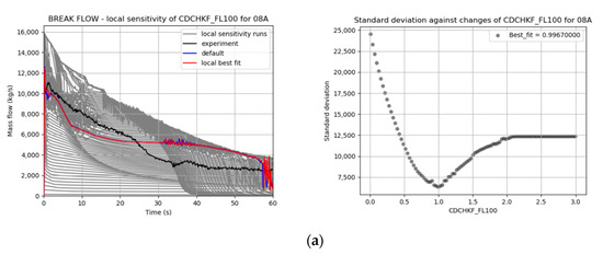
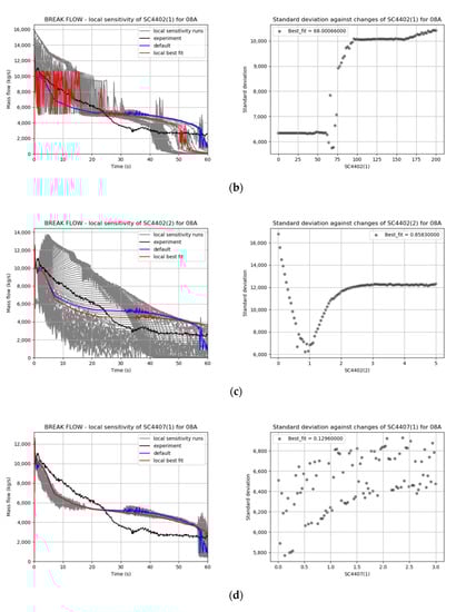
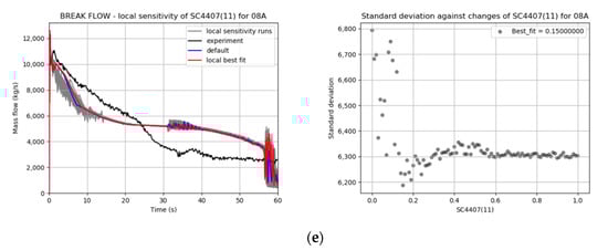
Figure 8.
Local sensitivity analysis for the chosen parameters for the 08A nodalization. (a–e) Different parameters: left—break flow and right—standard deviation for best-fit approach. CDCHKF_FL—Discharge Factor, SC4402(1)—Choking velocity limit, SC4402(2)—Moody model multiplication factor, SC4407(1)—Bubble rise velocity, and SC4407(11)—Maximum void fraction.
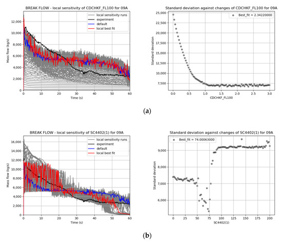
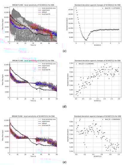
Figure 9.
The local sensitivity analysis for the chosen parameters for the 09A nodalization. (a–e) Different parameters: left—break flow and right—standard deviation for the best-fit approach. CDCHKF_FL—Discharge Factor, SC4402(1)—Choking velocity limit, SC4402(2)—Moody model multiplication factor, SC4407(1)—Bubble rise velocity, and SC4407(11)—Maximum void fraction.
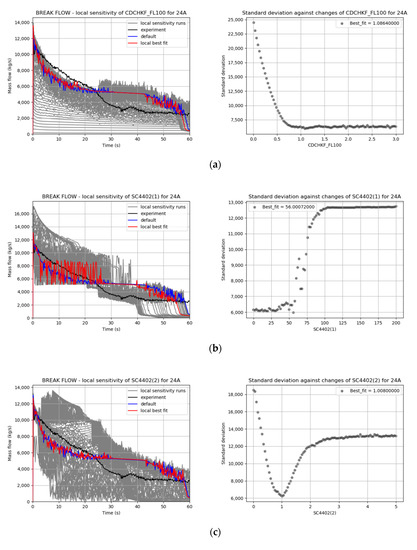
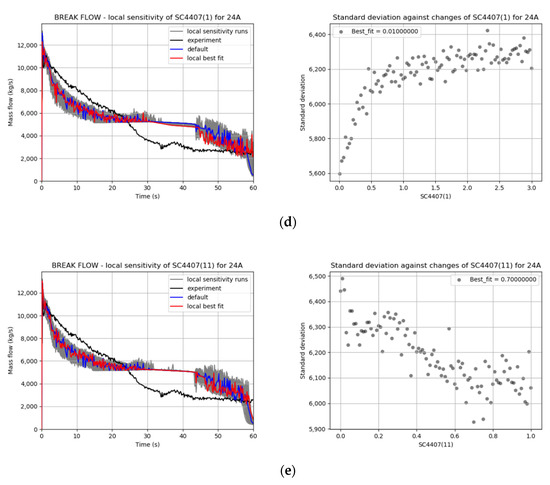
Figure 10.
The local sensitivity analysis for the chosen parameters for the 24A nodalization. (a–e) Different parameters: left—break flow and right—standard deviation for the best-fit approach. CDCHKF_FL—Discharge Factor, SC4402(1)—Choking velocity limit, SC4402(2)—Moody model multiplication factor, SC4407(1)—Bubble rise velocity, and SC4407(11)—Maximum void fraction.
Figure 8a–e, Left presents the changes of the mass flows through the break in respect to the time with the results for the experiment, default case, best-fit cases, and bundle of plots for the sensitivity cases for the 08A model. Figure 8a–e, Right shows the values of the standard deviations for all the runs for the subsequent local sensitivity parameters listed in Table 5. The discharge coefficient (CDCHKF)), whose optimum is 0.9967, slightly below the default value of 1.0 (Figure 8a, Right), has a significant influence on the results. Similarly, the choking flow-limiting velocity (SC4402(1)) has a substantial impact, showing unstable behavior over 60 m/s. However, this parameter for the best fit produces nonphysical results, as it is due to the numerical nature of this parameter. Figure 8c shows that the impact of the Moody multiplications factor (SC4402(2)) is also significant, with the best-fit value of 0.8583 being close to the default. The bubble rise velocity (SC4407(1)) has no effect in this case. Similarly, the maximum void fraction (SC4407(11)) has little importance, and above the value of ~0.3, it did not improve the results. The results obtained for 08A are stable, as only small numerical oscillations were observed.
In Figure 9a–e, Left are the changes of the mass flows through the break with respect to the time with the results for the experiment, default case, best-fit cases, and bundle of plots for sensitivity cases for the 09A model. Figure 9a–e, Right shows the values of the standard deviations for all the runs for the subsequent local sensitivity parameters listed in Table 5. The discharge coefficient (CDCHKF)), whose optimum is 2.3422, significantly above the default value of 1.0 (Figure 9a, Right), has a significant influence on the results. Increasing the CDCHKF value above 1.2 does not increase the break flow but generates oscillations greater in amplitude. The choking flow-limiting velocity (SC4402(1)) also substantially impacts the results, showing unstable behavior over 50 m/s. Again, the best-fit value of the parameter produces nonphysical results, as it is due to the numerical nature of this parameter. Figure 9c shows that the impact of the Moody multiplications factor (SC4402(2)) is also significant, with the best-fit value 1.2575 being close to the default. The bubble rise velocity (SC4407(1)) has no effect in this case. Similarly, the maximum void fraction (SC4407(11)) has little importance, and above the value of ~0.7, it did not improve the results. The results obtained for 09A are volatile, as lots of numerical oscillations were observed.
Comparing the results presented in Figure 9 with Figure 8, one may observe a significant difference in agreement with the experiment and the presence of oscillations for the 09A model. Using the 09A model with an additional CV for the nozzle did not improve the results but actually made them worse and less stable.
Figure 10a–e, Left presents the changes of the mass flows through the break with respect to the time with the results for the experiment, default case, best-fit cases, and bundle of plots for the sensitivity cases for the 24A model. Figure 10a–e, Right shows the values of the standard deviations for all the runs for the subsequent local sensitivity parameters listed in Table 5. The discharge coefficient (CDCHKF)), whose optimum is 1.0864, slightly above the default value of 1.0 (Figure 10a, Right), has a significant influence on the results. Similarly, the choking flow-limiting velocity (SC4402(1)) has a substantial impact, showing unstable behavior over 35 m/s. However, this parameter for the best fit produces nonphysical results, as observed in the previous cases. Figure 10c shows that the impact of the Moody multiplications factor (SC4402(2)) is also significant, with the best-fit value 1.008 very close to the default. The bubble rise velocity (SC4407(1)) has a negligible effect for this case, improving the results for values less than 0.1. Similarly, the maximum void fraction (SC4407(11)) has little importance. The results obtained for 24A are relatively not stable, as numerous numerical oscillations were observed.
3.3. Time of Calculations
The calculations were performed on a personal computer (i7-8700 CPU @ 3.20 GHz, 32.0 GB RAM). The computational time (CPU time) for each individual run of 60 s of the code calculations was determined.
The histograms of the computational time and median and mean for the models discussed in the previous section are presented in Figure 11. All individual runs—505 for each model—were taken into account to determine the CPU time for each nodalization. The highest median calculation time (294.83 s) was obtained for 24A nodalization and the lowest (0.75 s) for 01A nodalization. This comparison clearly shows to what extent the nodalization density impacts the calculation time, which, from the point of view of the analyses carried out at MELCOR, is often of decisive importance.
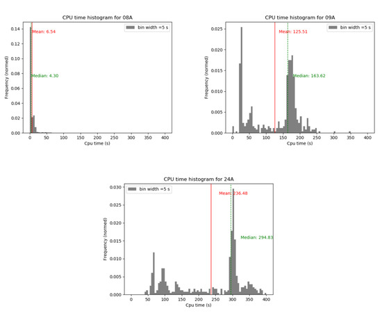
Figure 11.
Histogram of the CPU time for all the analyzed nodalizations.
The median CPU time for the model with a small CV for nozzle showed a much greater value than the nodalization with the same number of CVs but with a more balanced volume of individual CVs. These differences are clearly visible in the case of the nodalization of 02A (median 0.88 s) and 02C (median 17.47 s), the nodalization of 03A (median 5.77 s) and 03B (median 29.95 s), and the nodalization of 04A (median 7.66 s) and 04C (median 87.41 s). The same situation can be observed for 08A (median 4.33 s) and 09A (median 163.32 s), which are also similar in this regard. An obvious regularity was also noted that increasing the amount of CVs in the model increases the CPU time, i.e., based on the average from 0.75 s for 01A, by 0.87 s for 02A, 4.94 s for 03A, by 6.19 s for 04A, by 7.43 s for 06A, 6.54 s for 08A, and up to 236.48 s for 24A. Two nodalizations stand out from this set, i.e., 02A, which has a very fast computation time and satisfactory compliance with the experimental results, and a 08A nodalization with a good stability of the calculations, compatibility with the experiment, and quite short CPU time. Modifying the 08A model by adding a separate CV for the nozzle with a small volume (09A) resulted in a significant increase in the CPU time. Therefore, from the point of view of the calculation length, it is not recommended to use those nodalizations. Moreover, 09A is also less consistent with the experiment than 08A.
4. Conclusions
In this work, the MELCOR2.2 critical flow model performance was studied using Marviken CFT-21 as a source of the experimental data. A local sensitivity analysis was performed, which allowed for identifying which parameters potentially affect the flow rate during a critical flow. It allowed assessing the MELCOR default setup and to propose some best-fit parameters for the test CFT-21. Additionally, a unique method based on the regression analysis, which can be used to identify the best-fit parameters, was proposed and tested.
On the basis of the performed default model analysis and local sensitivity analysis, some recommendations and observations can be formulated. In the first observation, the presented results and method confirmed that the default values used in the MELCOR code for the critical flow allowed obtaining results the most consistent with the experimental data. In consequence, manipulations of the sensitivity coefficient should be limited.
The most basic (trivial) observation is that the choice of nodalization is important for critical flow modeling with MELCOR. Among all the studied models, nodalization with eight CVs (08A) proved to be the best and recommended. This nodalization was created using an approach assuming that the connecting CVs do not differ in volume by more than two (or less than 0.5). This allowed to obtain satisfactory results without oscillations and with a short CPU time. Furthermore, the strategy to avoid significant differences in the neighboring volumes proved to be efficient also for the other studied cases.
Regarding the nodalization for simple models, it was observed that, instead of using a model built of one CV, it is preferred to use two CV nodalizations. It can provide significantly better compatibility with the experiment while maintaining the stability of the calculations and short CPU time. The improvement of the nodalization by the addition of a CV with a small volume (like in this test case—CV representing the outlet nozzle) is not recommended. Nodalizations containing the unbalanced volume of CVs in the model resulted in the possibility of oscillations and a significant increase in the computational time. These observations can be applicable for simpler models with less nodes.
It can be concluded that guidance for critical flow modeling can be eventually applied to prepare a very detailed model of the pipework in a light water reactor, especially in the vicinity of the break. However, it has to be remembered that the typical light water reactors models in the MELCOR code have coarse nodalization and are rarely so detailed as the recommended model of 08A. It may be very difficult to apply the presented observations without substantially negative effects on the model convergence and computational time. Nevertheless, it may provide a good starting point for research activities focused on the critical flow in plant-scale conditions.
It was observed that the optimal value for the discharge coefficient (CDCHKF) is close to the value of 1.0, and for the best of the analyzed nodalizations, i.e., 08A, it was 0.9967. Taking small values of CDCHKF (i.e., less than approx. 0.5) causes a significant underestimation of the critical flow and, thus, a considerable inconsistency with the experiment results. Higher values of CDCHKF (i.e., greater than approx. 2.0) did not cause a further increase in the value of the flow rate.
Regardless of the nodding scheme, the optimal value of the multiplication factor for the Moody critical flow (SC4402(2)) is close to 1.0—the default value and the analyzed nodalizations determined the range of variation of this parameter to be 0.80–1.25. For most nodalizations (except 02C and 03B—which are not recommended), the values of the choking flow test velocity (SC4402(1)) below 25 m/s provide the best agreement with the experimental results. Based on the achieved results, it can be suggested that values of SC4402(1) lower than 25 should be used. It should be noted that the default value of SC4402(1) is 20.0, and according to the performed analysis, this value can be used in MELCOR calculations without any negative consequences.
For most nodalizations, assuming parameter SC4407(11) (maximum void fraction in a pool) values greater than approximately 0.7 had a positive effect on the compliance with the experiment results. In general, it should not be modified, and a low value can be set without substantial numerical problems.
The reader should also be aware of the fact that MELCOR is not able to reproduce the results of the CFT-21 test accurately. Basically, its mathematical models (Moody model) have limitations and create obstacles. Without code redevelopment, it will be difficult to obtain better results. It was especially evident for the two-phase critical flow part of the experiment. However, the reader should be aware of the fact that the results were based on the single data for test CFT-21.
This work showed that the developed best-fit approach could be helpful in finding the best parameters, and what is remarkable, it was able to reproduce the MELCOR default values in many studied cases, despite the code limitations and ability to reproduce the experimental data. Further research activities are necessary to improve and test the proposed best-fit approach.
It is recommended to repeat this work for more (or all) Marviken tests. It can be considered a large undertaking and potentially will be a matter of future research. It can be considered in applying the proposed regression-based method for each test phase (flashing and two-phase flow) separately, as it may improve the obtained results and be more appropriate for identifying the best-fit parameters.
The proposed parameter finding approach is expected to obtain more satisfactory results when applied to the study analytical models or codes (like TRACE or RELAP), which are more suited to predicting detailed thermal-hydraulic phenomena.
The outcomes of this work will be used in further studies focused on various sensitivity and uncertainty methods for the Marviken test and, also, in plant full-scale simulations with the MELCOR code.
Author Contributions
Conceptualization, M.W.; Data curation, M.W. and P.D. (Paweł Domitr); Formal analysis, M.W. and P.D. (Paweł Domitr); Investigation, M.W., P.D. (Paweł Domitr), and P.D. (Piotr Darnowski); Methodology, M.W. and P.D. (Piotr Darnowski); Project administration, M.W.; Resources, M.W. and P.D. (Paweł Domitr); Software, M.W.; Supervision, M.W. and P.D. (Piotr Darnowski); Validation, M.W. and P.D. (Paweł Domitr); Visualization, M.W. and P.D. (Paweł Domitr); Writing—original draft, M.W., P.D. (Paweł Domitr), and P.D. (Piotr Darnowski); and Writing—review and editing, M.W., P.D. (Paweł Domitr), and P.D. (Piotr Darnowski). All authors have read and agreed to the published version of the manuscript.
Funding
This project was prepared as a part of the 2nd and 3rd editions of the implementation doctorates programme, the party of which is the National Atomic Energy Agency (Państwowa Agencja Atomistyki), as the employer of the first two authors. Warsaw University of Technology is host academic institution. The Polish Ministry of Education and Science provided the funding for this programme. The APC was funded by Warsaw University of Technology—Program Open Science IDUB.
Institutional Review Board Statement
Not applicable.
Informed Consent Statement
Not applicable.
Data Availability Statement
Data is available on demand.
Acknowledgments
The third Author would like to acknowledge National Atomic Energy Agency for support of Nuclear Energy research at Warsaw University of Technology.
Conflicts of Interest
The authors declare no conflict of interest.
References
- Humphries, L.L.; Cole, R.K.; Louie, D.L.; Figueroa, V.G.; Young, M.F. MELCOR 2.2 Computer Code Manual—Volume 1—Primer and Users’ Guide; Sandia National Laboratories: Albuquerque, NM, USA, 2017. [Google Scholar]
- Humphries, L.L.; Cole, R.K.; Louie, D.L.; Figueroa, V.G.; Young, M.F. MELCOR 2.2 Computer Code Manual—Volume 2—Reference Manual; Sandia National Laboratories: Albuquerque, NM, USA, 2017. [Google Scholar]
- Sandia National Laboratories. MELCOR 2.1 Computer Code Manual—Volume 3: MELCOR Assessment Problems; Sandia National Laboratories: Albuquerque, NM, USA, 2015.
- Sehgal, B.R. Nuclear Safety in Light Water Reactors Severe Accident Phenomeneology; Academic Press Elsevier: Cambridge, MA, USA, 2012. [Google Scholar]
- IRSN. Nuclear Power Reactor Core Melt Accidents; EDP Sciences: Paris, France, 2015.
- Salomon, L.; Levy, S. Two-Phase Flow in Complex Systems; John Wiley& Sons, Inc.: Hoboken, NJ, USA, 1999. [Google Scholar]
- Todreas, N.E.; Kazimi, M.S. Nuclear Systems I: Thermal Hydraulic Fundamentals; Taylor and Francis: Boca Raton, FL, USA, 2011. [Google Scholar]
- Anglart, H. Thermal Hydraulics in Nuclear Systems; Warsaw University of Technology Publishing Office: Warsaw, Poland, 2013. [Google Scholar]
- D’Auria, F. Thermal Hydraulics in Water-Cooled Nuclear Reactors; Elsevier: Cambridge, MA, USA, 2017. [Google Scholar]
- Lanfredini, M.; Bestion, D.; D’Auria, F.; Aksan, N.; Fillion, P.; Gaillard, P.; Heo, J.; Karppinen, I.; Kim, K.D.; Kurki, J.; et al. Critical flow prediction by system codes—Recent analyses made within the FONESYS network. Nucl. Eng. Des. 2020, 366, 110731. [Google Scholar] [CrossRef]
- Lee, I.; Oh, D.; Bang, Y.; Kim, Y. Effect of critical flow model in MARS-KS code on uncertainty quantification of large break Loss of coolant accident (LBLOCA). Nucl. Eng. Technol. 2020, 52, 755–763. [Google Scholar] [CrossRef]
- INL. RELAP5/MOD3 Code Manual; Idaho National Laboratory: Idaho Falls, ID, USA, 2010.
- U.S. Nuclear Regulatory Comission; U.S. NRC. TRACE V5.0 PATCH 5 THEORY MANUAL Field Equations, Solution Methods, and Physical Models; Office of Nuclear Regulatory Research: Washington, DC, USA, 2013.
- U.S. Nuclear Regulatory Comission. TRACE V5.840 User’s Manual Volume 2: Modeling Guidelines; Office of Nuclear Regulatory Research: Washington, DC, USA, 2014.
- U.S. Nuclear Regulatory Comission. TRACE V5.0 Assessment Manual—Appendix B: Separate Effects Tests; Office of Nuclear Regulatory Research: Washington, DC, USA, 2013.
- Geffraye, G.; Antoni, O.; Farvacque, M.; Kadri, D.; Lavialle, G.; Rameau, B.; Ruby, A. CATHARE 2 V2.5_2: A single version for various applications. Nucl. Eng. Des. 2011, 241, 4456–4463. [Google Scholar] [CrossRef]
- Sokolowski, L.; Kozlowski, T. Assessment of Two-Phase Critical Flow Models Performance in RELAP5 and TRACE Against Marviken Critical Flow Tests; Office of Nuclear Regulatory Research: Washington, DC, USA, 2012. [Google Scholar]
- D’Auria, F. Best Estimate Plus Uncertainty (BEPU): Status and perspectives. Nucl. Eng. Des. 2019, 352, 110190. [Google Scholar] [CrossRef]
- Tills, J. MELCOR DBA Containment Audit Calculations for the ESBWR Plant; Sandia National Laboratories: Albuquerque, NM, USA, 2010. [Google Scholar]
- Tills, J.; Notafrancesco, A.; Phillips, J.; SNL. SAND2009-2858. In Application of the MELCOR Code to Design Basis PWR Large Dry Containment Analysis; Sandia National Laboratories: Albuquerque, NM, USA, 2009. [Google Scholar]
- Clement, B.; Haste, T. Thematic Network for a Phebus FPT-1 International Standard Problem—Comparison Report on International Standard Problem ISP-46; OECD/NEA Report; OECD Nuclear Energy Agency: Issy-les-Moulineaux, France, 2003. [Google Scholar]
- Gauntt, R.; Bixler, N.E.; Wagner, K.C. An Uncertainty Analysis of the Hydrogen Source Term for a Station Blackout Accident in Sequoyah Using MELCOR 1.8.5; Sandia National Laboratories: Albuquerque, NM, USA, 2014. [Google Scholar]
- Spirzewski, M.; Domitr, P.; Darnowski, P. Global uncertainty and sensitivity analysis of MELCOR and TRACE critical flow models against MARVIKEN tests. Nucl. Eng. Des. 2021, 378, 111150. [Google Scholar] [CrossRef]
- Domitr, P.; Darnowski, P.; Spirzewski, M. The Assessment of Critical Flow Models of MELCOR2.2 and TRACE V5.0 Patch 5 against MARVIKEN Critical Flow Tests. In Proceedings of the 18th International Topical Meeting on Nuclear Reactor Thermal Hydraulics NURETH 2019, Portland, OR, USA, 18–23 August 2019. [Google Scholar]
- Mosunova, N. MELCOR 2.1 Verification on MARVIKEN Critical Flow Experiments; European Melcor User Group Meeting EMUG-2013: Stockholm, Sweden, 2013. [Google Scholar]
- Marviken Project. The Marviekn Full Scale Critical Flow Tests Report; OECD: Paris, France; NEA: Paris, France, 1979. [Google Scholar]
- Homenda, W.; Pedrycz, W. Pattern Recognition—A Quality of Data Perspective; Wiley: Hoboken, NJ, USA, 2018. [Google Scholar]
- Humphries, L. MELCOR Code Development Status Presented by Larry Humphries European MELCOR User Group Held May 2–3, 2013 in Stockholm, Sweden. 2013. Available online: https://www.osti.gov/servlets/purl/1078970 (accessed on 1 July 2021).
Publisher’s Note: MDPI stays neutral with regard to jurisdictional claims in published maps and institutional affiliations. |
© 2021 by the authors. Licensee MDPI, Basel, Switzerland. This article is an open access article distributed under the terms and conditions of the Creative Commons Attribution (CC BY) license (https://creativecommons.org/licenses/by/4.0/).