
A Step-by-Step Procedure to Perform Preliminary Designs of Salient-Pole Synchronous Generators


Abstract
:
1. Introduction
2. Materials and Methods
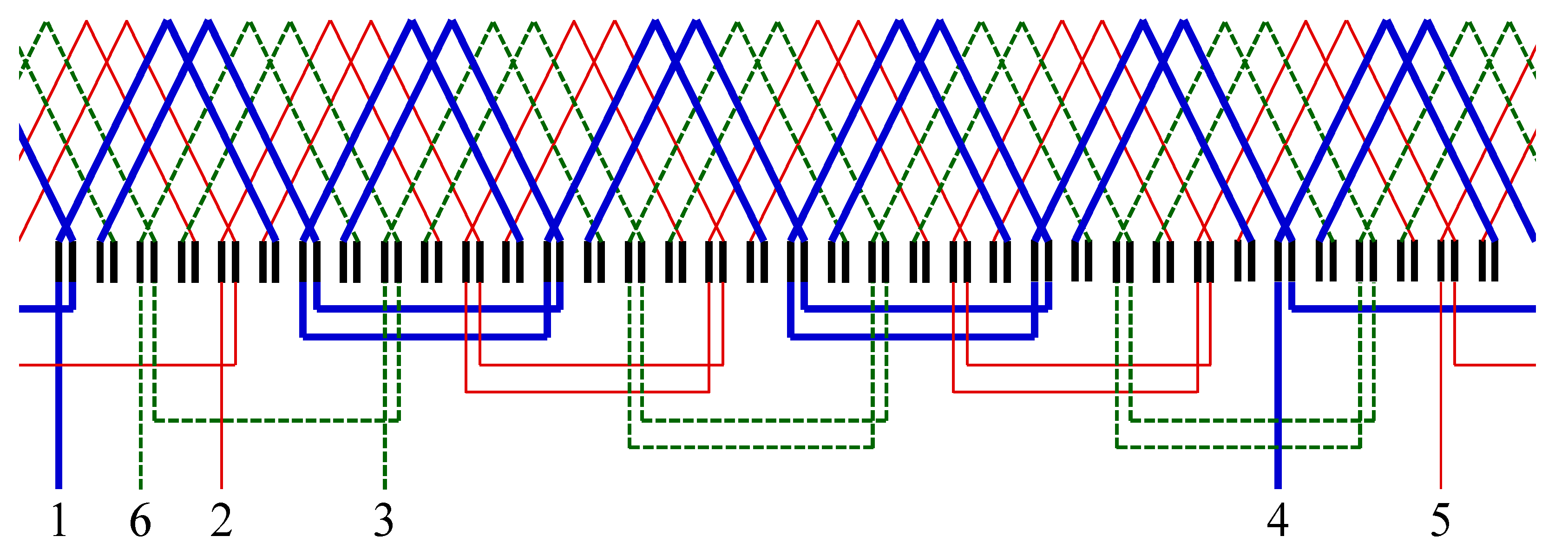
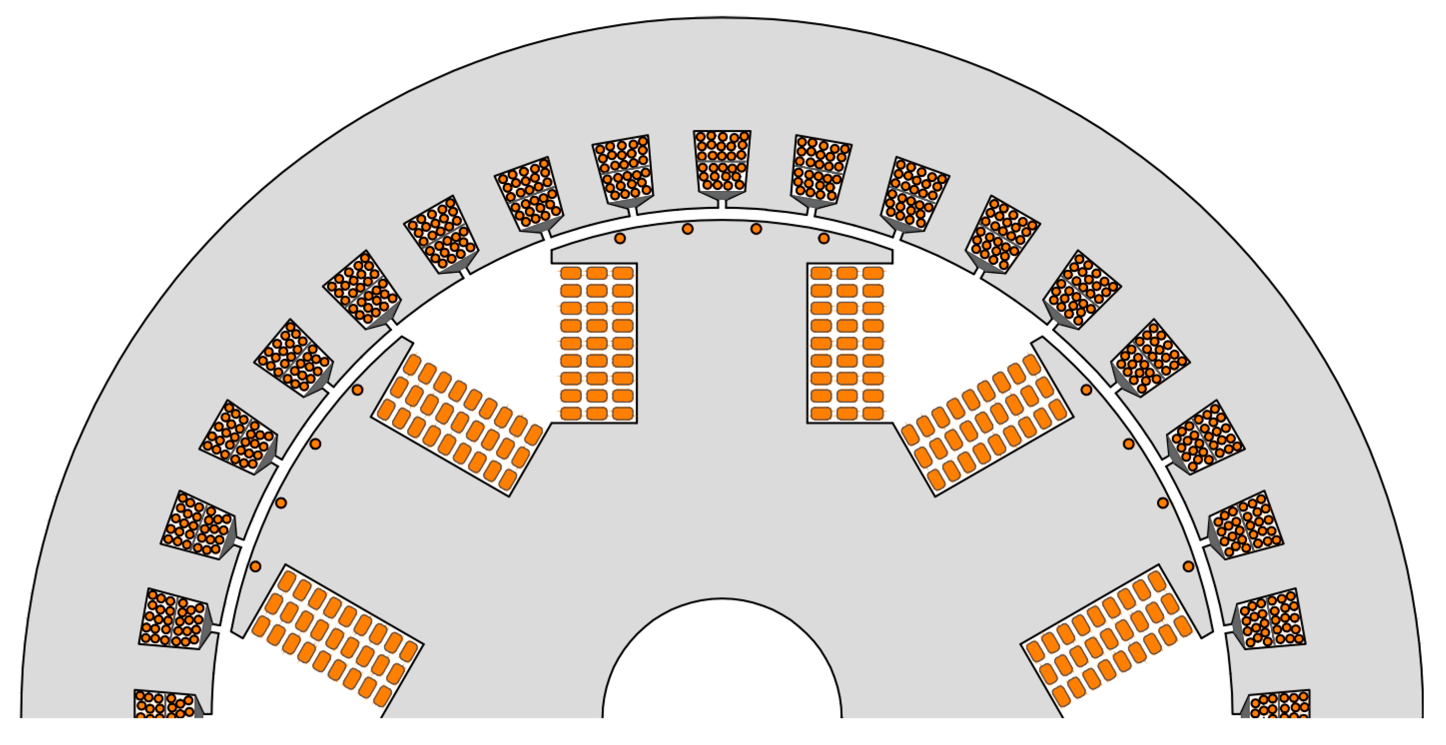
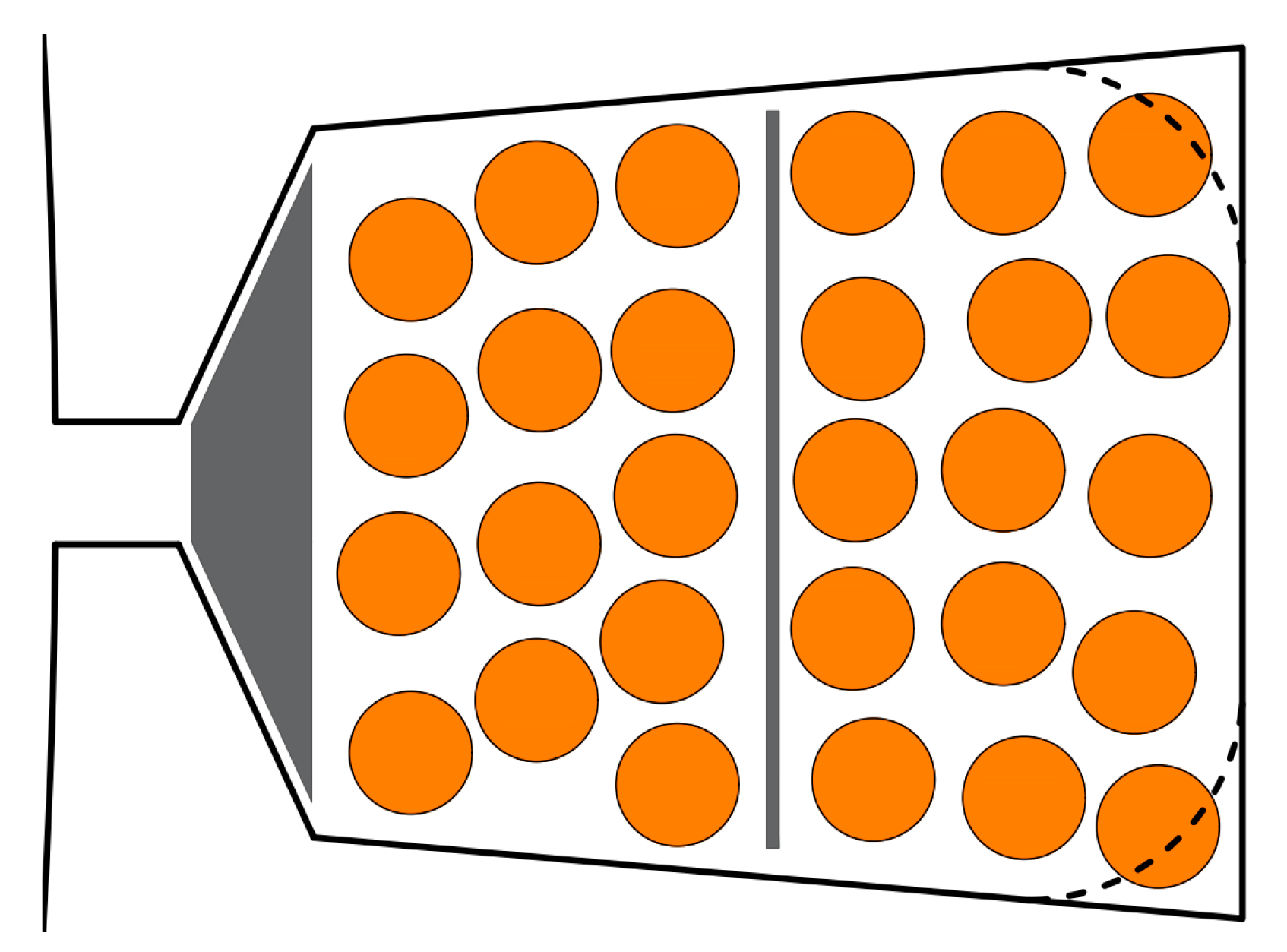
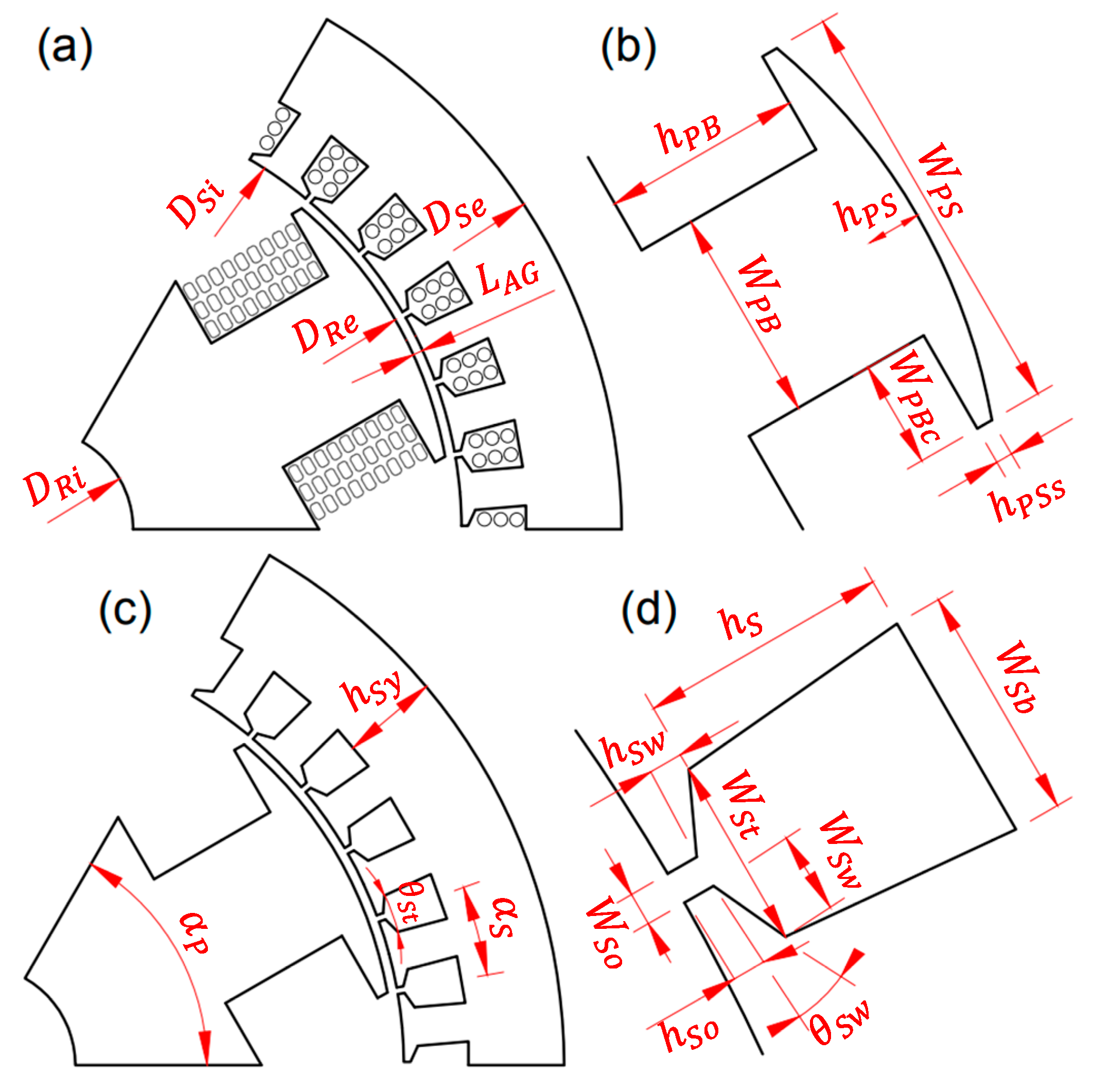
2.1. Generator Topology
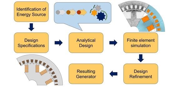
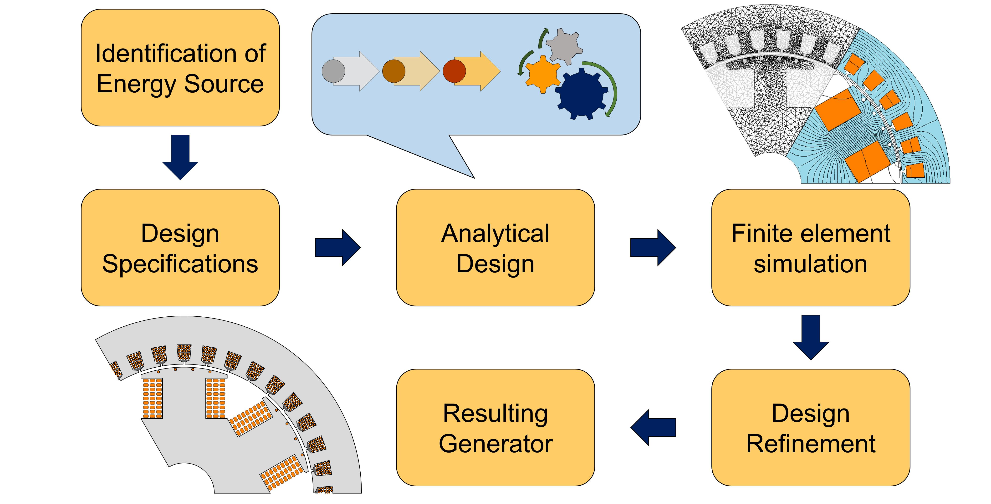
2.2. General Design Flow

| Symbol | Unit | Description | Value |
|---|---|---|---|
| VA | Desired Output Power | 15,000 | |
| V | Desired Terminal Voltage | 400 | |
| - | Power Factor | 0.9 | |
| Hz | Electrical frequency | 50 | |
| rpm | Rotation | 1000 |
| Symbol | Unit | Suggested Values 1/Ranges | Value |
|---|---|---|---|
| mm | 2 | 250 | |
| - | 1/2–5/6 | 2/3 | |
| - | 1/3–3/4 | 4/11 | |
| - | 0.12–0.2 | 0.15 | |
| A | 4–7.5 | 5 | |
| A/mm² | 2–3.5 [1] | 3 | |
| - | 0.5–0.9 | 0.8 | |
| ≈1.5/100 of 3 | 3.5 | ||
| mm | 2 | 200.2 | |
| - | 0.95–1.15 | 1.023 | |
| A | ≈50% of | 2.5 | |
| - | 4 | 2 | |
| mm | ≈ | 2 | |
| mm | 5 | 2.24 | |
| - | 0.85–1.15 | 1 | |
| - | 0.5–1.5 | 4/5 | |
| - | 1/3–5/6 | 0.692 | |
| - | 5/6 or 2/3 | 5/6 | |
| slots | 6 | 36 | |
| paths | number of poles | 6 | |
| layers | 1 or 2 | 2 | |
| - | 0.75–0.95 [2] | 0.89 | |
| - | 1/3–2/3 7 | 0.5 | |
| A | 8 | 2.5 | |
| A | 8 | 4.78 | |
| Ω/km | 9 | 3.92 | |
| Ω/km | 10 | 10.30 | |
| A/mm² | 4–6.5 [1] | 5 | |
| - | 1/3–1/1 | 4/5 | |
| - | 0.8–0.9 or 1.1–1.2 [1] | 0.8 | |
| - | 0.1–0.3 [1] | 0.1 | |
| W/kg | 1.656 [21] | 1.656 | |
| W/kg | 0.698 [21] | 0.698 |
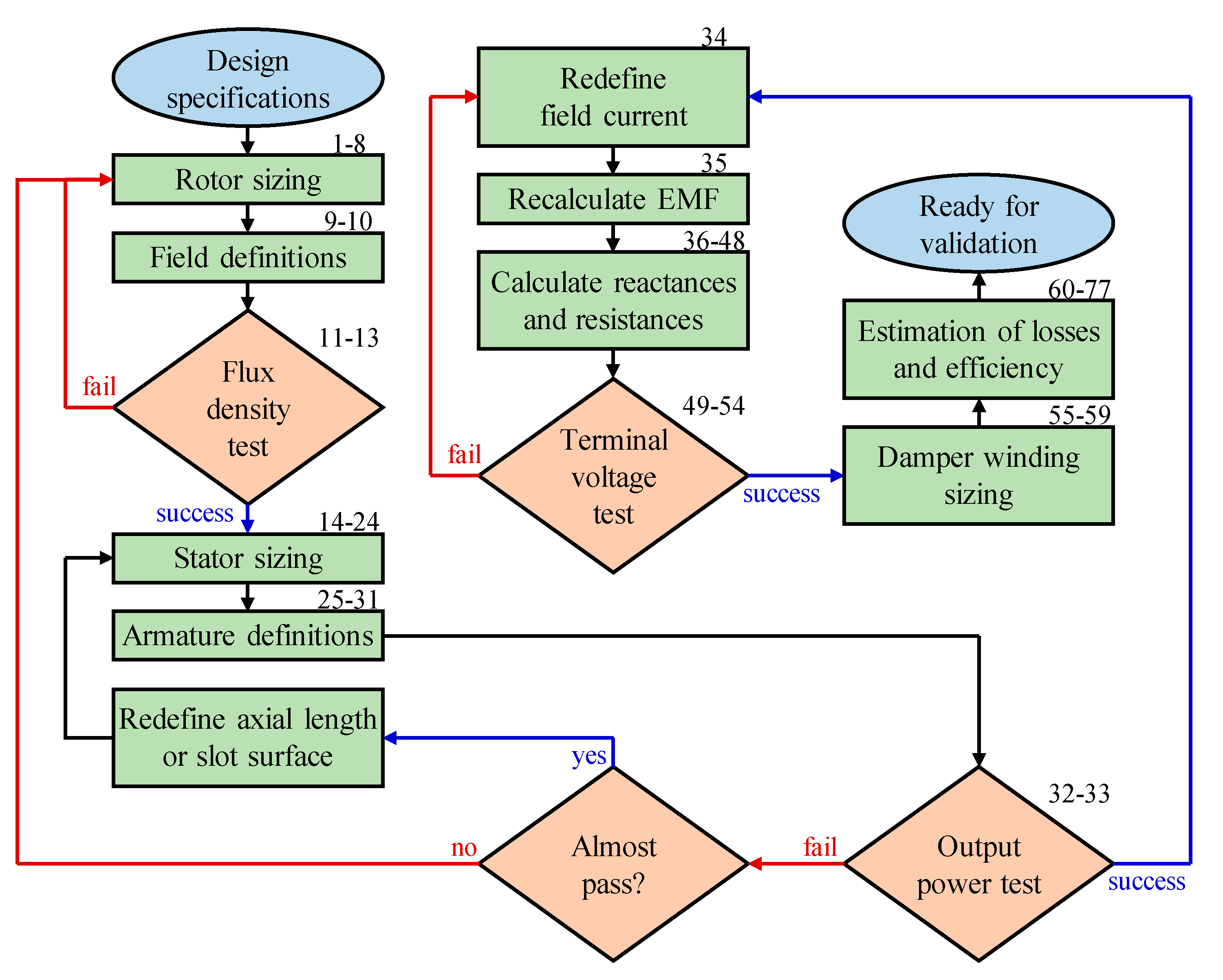
2.3. Step-by-Step Design Procedure
2.3.1. No-Load Design
Rotor Design
Stator Design
2.3.2. Full-Load Design
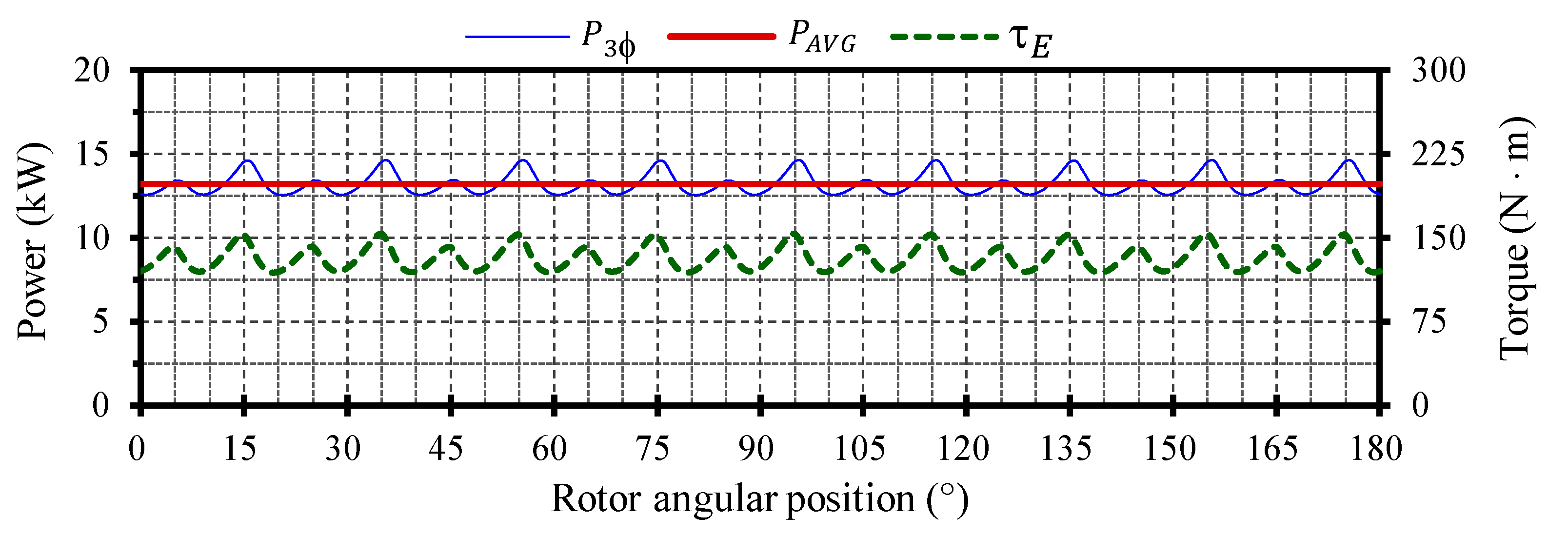
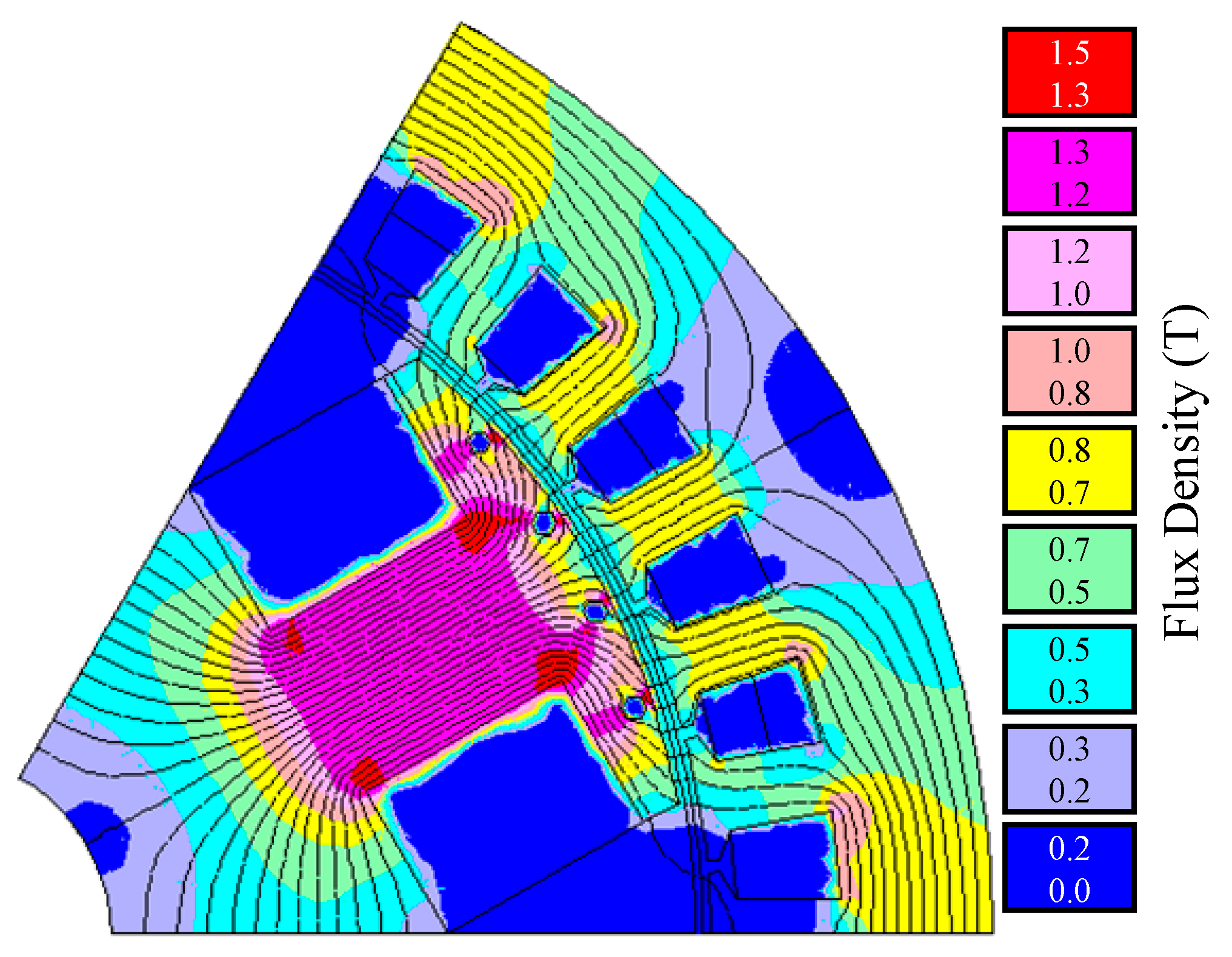
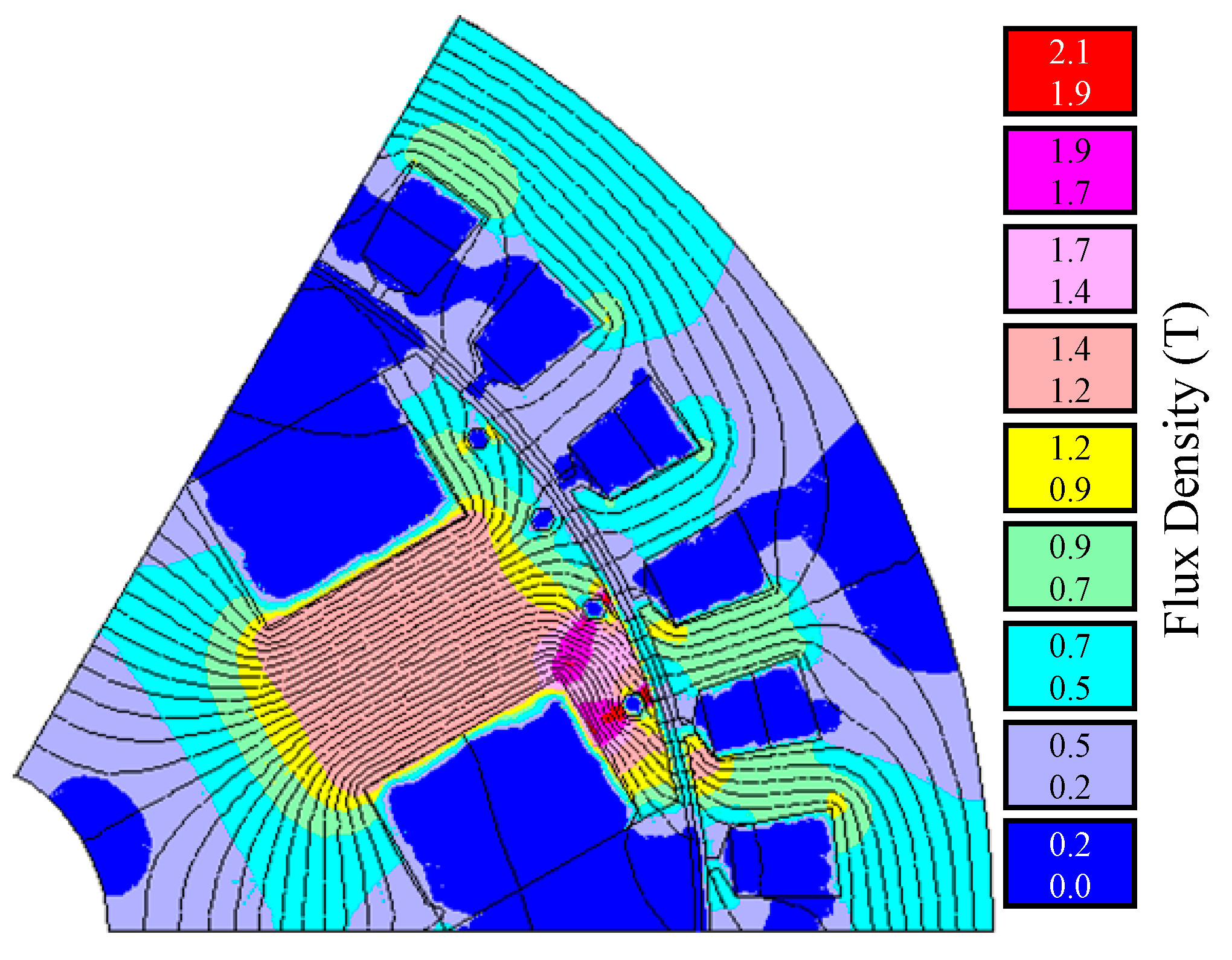
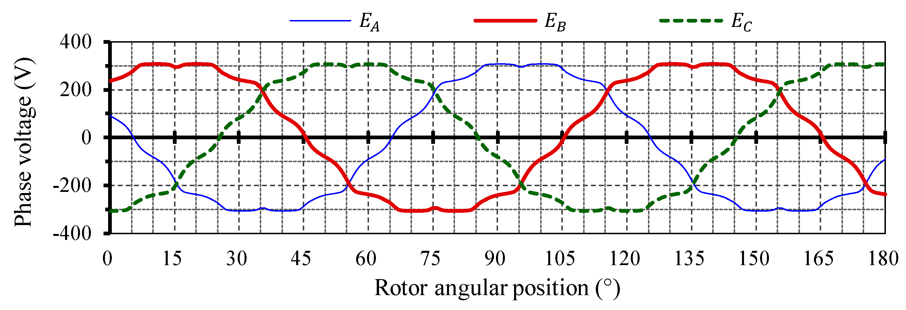
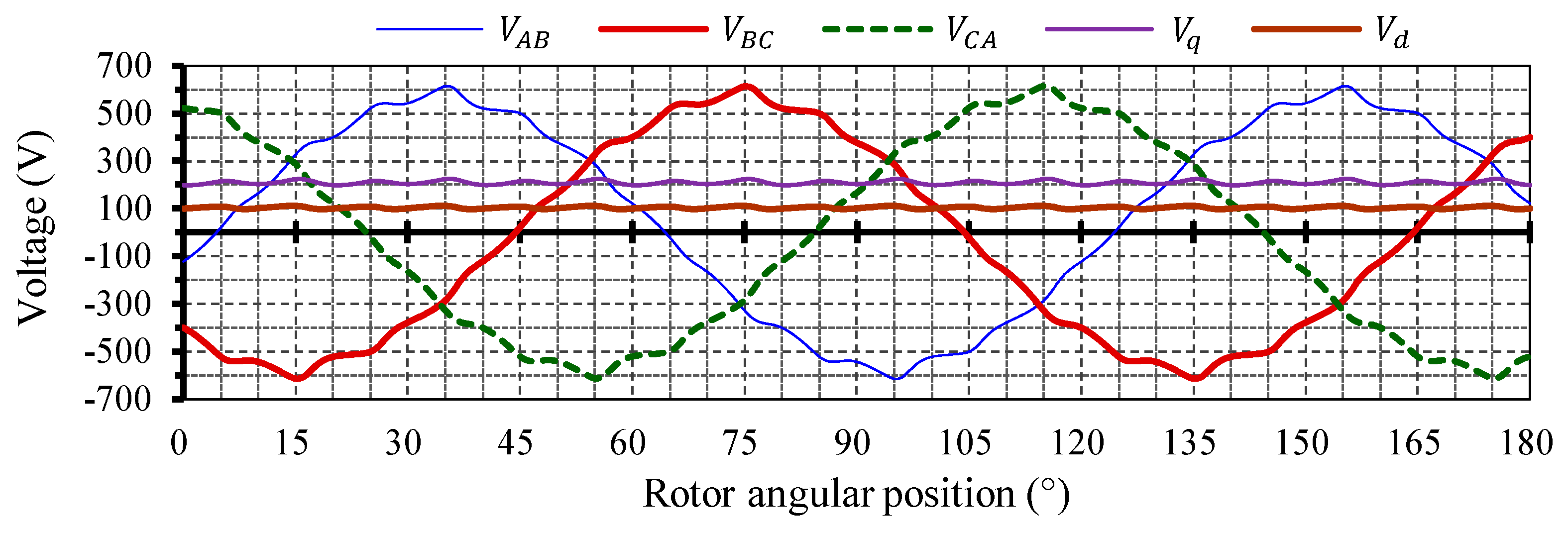
3. Results and Discussions
- As the iron core reluctance is neglected, the flux density has been kept low;
- Narrow slots have been avoided to minimize flux leakage.
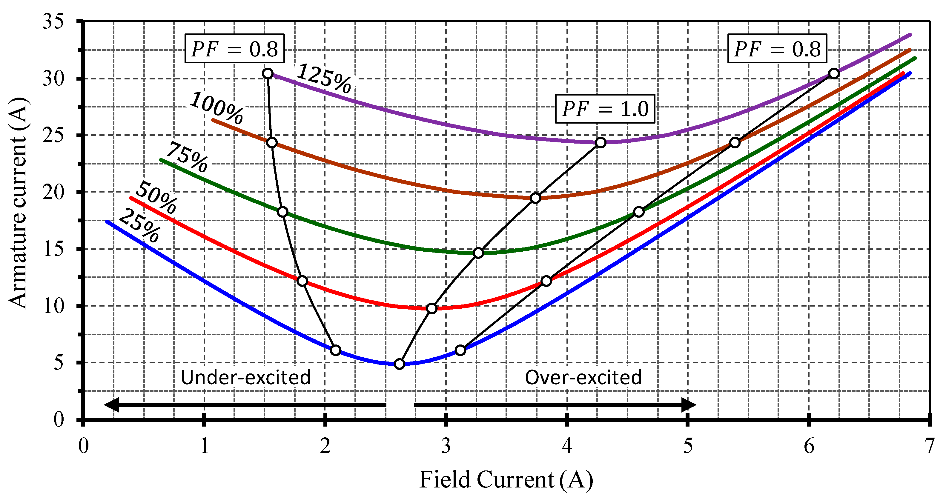
- A new magnitude of armature current is imposed in step 32, corresponding to 25%, 50%, 75%, 100%, and 125% loads;
- The value of the field current is adjusted to keep the terminal voltage constant at 400 V;
- The values of direct and quadrature axis reactances, used in steps 49, 52, and 53, as well as the power factor, are considered constants;
- The load angle value, corresponding to each load condition, is calculated by (49).
Discussions about Improvements in the Design
4. Conclusions
Author Contributions
Funding
Conflicts of Interest
References
- Pyrhönen, J.; Jokinen, T.; Hrabovcova, V. Design of Rotating Electrical Machines, 1st ed.; John Wiley & Sons: Chichester, UK, 2008. [Google Scholar]
- Boldea, I. Synchronous Generators, 2nd ed.; CRC Press: Boca Raton, FL, USA, 2016. [Google Scholar]
- Hendershot, J.R.; Miller, T.J.E. Design of Brushless Permanent-Magnet Machines, 1st ed.; Motor Design Books: Venice, CA, USA, 2010. [Google Scholar]
- Hanselman, D.C. Brushless Permanent Magnet Motor Design, 2nd ed.; The Writers’ Collective: Cranston, RI, USA, 2003. [Google Scholar]
- Bazzo, T.P.M.; Kölzer, J.F.; Carlson, R.; Wurtz, F.; Gerbaud, L. Multiphysics Design Optimization of a Permanent Magnet Synchronous Generator. IEEE Trans. Ind. Electron. 2017, 64, 9815–9823. [Google Scholar] [CrossRef]
- Bernard, N.; Missoum, R.; Dang, L.; Bekka, N.; Ahmed, H.B.; Zaïm, M.E. Design Methodology for High-Speed Permanent Magnet Synchronous Machines. IEEE Trans. Energy Convers. 2016, 31, 477–485. [Google Scholar] [CrossRef] [Green Version]
- Bianchi, N.; Bolognani, S.; Pre, M.D.; Bekka, N.; Grezzani, G. Design considerations for fractional-slot winding configurations of synchronous machines. IEEE Trans. Ind. Appl. 2006, 42, 997–1006. [Google Scholar] [CrossRef]
- Laldin, O.; Sudhoff, S.D.; Pekarek, S. An Analytical Design Model for Wound Rotor Synchronous Machines. IEEE Trans. Energy Convers. 2015, 30, 1299–1309. [Google Scholar] [CrossRef]
- Nardo, M.D.; Calzo, G.L.; Galea, M.; Gerada, C. Design Optimization of a High-Speed Synchronous Reluctance Machine. IEEE Trans. Ind. Appl. 2018, 54, 233–243. [Google Scholar] [CrossRef]
- Yang, C.; Lin, H.; Guo, J.; Zhu, Z.Q. Design and Analysis of a Novel Hybrid Excitation Synchronous Machine with Asymmetrically Stagger Permanent Magnet. IEEE Trans. Magn. 2008, 44, 4353–4356. [Google Scholar] [CrossRef]
- Daghigh, A.; Javadi, H.; Torkaman, H. Optimal Design of Coreless Axial Flux Permanent Magnet Synchronous Generator with Reduced Cost Considering Improved PM Leakage Flux Model. Electr. Power Compon. Syst. 2017, 45, 264–278. [Google Scholar] [CrossRef]
- Kim, H.; Jeong, J.; Yoon, M.; Moon, J.; Hong, J. Simple Size Determination of Permanent-Magnet Synchronous Machines. IEEE Trans. Ind. Electron. 2017, 64, 7972–7983. [Google Scholar] [CrossRef]
- Hebala, A.; Ghoneim, W.A.M.; Ashour, H.A. Detailed Design Procedures for PMSG Direct-Driven by Wind Turbines. J. Electr. Eng. Technol. 2019, 14, 251–263. [Google Scholar] [CrossRef]
- Vaschetto, S.; Tenconi, A.; Bramerdorfer, G. Sizing procedure of surface mounted PM machines for fast analytical evaluations. In Proceedings of the IEEE International Electric Machines and Drives Conference (IEMDC), Miami, FL, USA, 21–24 May 2017; IEEE: Piscataway, NJ, USA, 2017. [Google Scholar] [CrossRef]
- Uzhegov, N.; Kurvinen, E.; Nerg, J.; Pyrhönen, J.; Sopanen, J.T.; Shirinskii, S. Multidisciplinary Design Process of a 6-Slot 2-Pole High-Speed Permanent-Magnet Synchronous Machine. IEEE Trans. Ind. Electron. 2016, 63, 784–795. [Google Scholar] [CrossRef]
- Xiao, Y.; Zhou, L.; Wang, J.; Yang, R. Finite Element Computation of Transient Parameters of a Salient-Pole Synchronous Machine. Energies 2017, 10, 1015. [Google Scholar] [CrossRef] [Green Version]
- Jones, C.V. The Unified Theory of Electrical Machines, 1st ed.; Butterworths: London, UK, 1967. [Google Scholar]
- Shima, K.; Ide, K.; Takahashi, M. Finite-element calculation of leakage inductances of a saturated salient-pole synchronous machine with damper circuits. IEEE Trans. Energy Convers. 2002, 17, 463–470. [Google Scholar] [CrossRef]
- Misir, O.; Raziee, S.M.; Ponick, B. Determination of the Inductances of Salient Pole Synchronous Machines Based on the Voltage Equation of a Single Coil in the Stator Winding. IEEE Trans. Ind. Appl. 2016, 52, 3792–3804. [Google Scholar] [CrossRef]
- Tessarolo, A. Accurate Computation of Multiphase Synchronous Machine Inductances Based on Winding Function Theory. IEEE Trans. Energy Convers. 2012, 27, 895–904. [Google Scholar] [CrossRef]
- Grauers, A. Design of Direct-Driven Permanent-Magnet Generators for Wind Turbines, in School of Electrical and Computer Engineering; Chalmers University of Technology: Göteborg, Sweden, 1996. [Google Scholar]
- Krause, P.C.; Wasynczuk, O.; Sudhoff, S. Analysis of Electric Machinery and Drive Systems, 2nd ed.; IEEE Press Power Engineering Series: Danvers, MA, USA, 2002. [Google Scholar]
- Wang, Y.; Nuzzo, S.; Gerada, C.; Zhao, W.; Zhang, H.; Galea, M. 3D Lumped Parameter Thermal Network for Wound-Field Synchronous Generators. In Proceedings of the IEEE Workshop on Electrical Machines Design, Control and Diagnosis (WEMDCD), Modena, Italy, 8–9 April 2021; IEEE: Piscataway, NJ, USA, 2021. [Google Scholar] [CrossRef]
- Ghahfarokhi, P.S.; Kallaste, A.; Podgornov, A.; Belahcen, A.; Vaimann, T.; Kudrjavtsev, O. Thermal Analysis of Salient Pole Synchronous Machines by Multiple Model Planes Approach. In Proceedings of the International Conference on Electrical Machines (ICEM), Gothenburg, Sweden, 23–26 August 2020; IEEE: Piscataway, NJ, USA, 2020. [Google Scholar] [CrossRef]


| Symbol | Unit | Description | Value |
|---|---|---|---|
| poles | Number of poles | 6 | |
| mm | Width of pole shoes | 85.51 | |
| mm | Width of pole body | 31.09 | |
| mm | Height of pole shoes | 13.81 | |
| mm | Height of pole body | 37.14 | |
| mm² | Surface of field conductor | 1.67 | |
| turns | Field winding turns | 485 | |
| mm | Internal diameter of stator | 257 | |
| mm | Top of slot width | 11.59 | |
| mm | Bottom of slot width | 14.60 | |
| mm | Height of the slot | 17.20 | |
| mm | Height of stator yoke | 24.87 | |
| mm | External diameter of stator | 349.6 | |
| coils | Number of coils per pole and per phase | 2 | |
| turns | Number of turns per coil | 13 | |
| mm² | Armature conductor surface | 4.33 | |
| mm | Diameter of damper bars | 4.64 | |
| bars | Number of damper bars per pole | 4 | |
| mH | Direct axis inductance 1 | 40.78 | |
| mH | Quadrature axis inductance 1 | 26.10 | |
| mH | End-winding inductance | 1.18 | |
| Ω | Direct axis reactance | 13.18 | |
| Ω | Quadrature axis reactance | 8.57 | |
| Ω | Armature resistance per phase 2 | 0.6275 | |
| Ω | Field resistance 2 | 3.80 |
| Symbol | Unit | Description | Value |
|---|---|---|---|
| W | Armature copper losses | 883.0 | |
| W | Field copper losses | 87.5 | |
| W | Stator yoke core losses due to hysteresis | 45.6 | |
| W | Stator yoke core losses due to Foucault | 17.3 | |
| W | Stator teeth core losses due to hysteresis | 67.6 | |
| W | Stator yoke core losses due to Foucault | 59.3 | |
| W | Windage and ventilation losses | 119.4 | |
| W | Total losses | 1282.3 | |
| η | % | Estimated efficiency | 91.3 |
| Loading | Armature Current | Field Current | Load Angle |
|---|---|---|---|
| 25% | 5.41 A | 2.94 A | 9.00° |
| 50% | 10.83 A | 3.49 A | 16.19° |
| 75% | 16.24 A | 4.11 A | 21.89° |
| 100% | 21.66 A | 4.78 A | 26.43° |
| 125% | 27.07 A | 5.47 A | 30.10° |
| Symbol | Unit | Design | FEA | diff. (%) |
|---|---|---|---|---|
| 1 | T | 1.25 | 1.28 | −2.3 |
| V | 400.3 | 405.98 | −1.4 | |
| A | 21.66 | 21.19 | +2.2 | |
| 2 | kVA | 15.01 | 14.90 | +0.7 |
| 3 | kW | 13.50 | 13.22 | +2.1 |
| PF 4 | - | 0.90 | 0.89 | +1.1 |
Publisher’s Note: MDPI stays neutral with regard to jurisdictional claims in published maps and institutional affiliations. |
© 2021 by the authors. Licensee MDPI, Basel, Switzerland. This article is an open access article distributed under the terms and conditions of the Creative Commons Attribution (CC BY) license (https://creativecommons.org/licenses/by/4.0/).
Share and Cite
Bazzo, T.d.P.M.; Moura, V.d.O.; Carlson, R. A Step-by-Step Procedure to Perform Preliminary Designs of Salient-Pole Synchronous Generators. Energies 2021, 14, 4989. https://doi.org/10.3390/en14164989
Bazzo TdPM, Moura VdO, Carlson R. A Step-by-Step Procedure to Perform Preliminary Designs of Salient-Pole Synchronous Generators. Energies. 2021; 14(16):4989. https://doi.org/10.3390/en14164989
Chicago/Turabian StyleBazzo, Thiago de Paula Machado, Vinicius de Oliveira Moura, and Renato Carlson. 2021. "A Step-by-Step Procedure to Perform Preliminary Designs of Salient-Pole Synchronous Generators" Energies 14, no. 16: 4989. https://doi.org/10.3390/en14164989
APA StyleBazzo, T. d. P. M., Moura, V. d. O., & Carlson, R. (2021). A Step-by-Step Procedure to Perform Preliminary Designs of Salient-Pole Synchronous Generators. Energies, 14(16), 4989. https://doi.org/10.3390/en14164989