Which Strategy Saves the Most Energy for Stratified Water Heaters?

Abstract

The operation of water heating uses a substantial amount of energy and is responsible for 30% of a household’s overall electricity consumption. Determining methods of reducing energy demand is crucial for countries such as South Africa, where energy supply is almost exclusively electrical, 88% of it is generated by coal, and energy deficits cause frequent blackouts. Decreasing the energy consumption of tanked water heaters can be achieved by reducing the standing losses and thermal energy of the hot water used. In this paper, we evaluate various energy-saving strategies that have commonly been used and determine which strategy is best. These strategies include optimising the heating schedule, lowering the set-point temperature, reducing the volume of hot water used, and installing additional thermal insulation. The results show that the best strategy was providing optimal control of the heating element, and savings of 16.3% were achieved. This study also determined that the magnitude of energy savings is heavily dependent on a household’s water usage intensity and seasonality.

1. Introduction

An electric water heater (EWH) uses a substantial amount of electricity and contributes to 30% of a household’s energy consumption [1]. Taking South Africa as an example, the country’s electricity generation is heavily dependent on fossil fuels, and 88% of the total generation is supplied by the burning of coal [2]. The country also struggles to meet the energy demand on the grid and has given rise to planned power outages (locally referred to as loadshedding), which is expected to continue for another five years [3]. Therefore, minimising energy costs of an EWH is directly linked to reducing the intensity of energy demand and greenhouse-gas emissions [4,5]. Even though studies that relate to smart grid applications have provided an in-depth analysis of thermal models and control algorithms, few of these models are explicitly designed to achieve an overall reduction in energy usage [6,7,8,9].

It is important to understand the fundamental processes of an EWH before energy-reducing strategies are proposed. A heating element supplies electrical energy to the tank to gradually increase the temperature, and consequently the thermal energy, of the water. The thermal energy that is stored in the EWH is reduced in two ways: The first way is caused by standing losses and refers to the loss of thermal energy from the water inside the tank to the environment due to the temperature difference. The rate of energy loss is also influenced by the thermal resistance of the tank. The second way is caused when energy is used from the tank in the form of water drawn at a higher temperature and the cold water then replacing it. The energy savings of an EWH are determined by environmental factors, the physical properties of the EWH, installation, configuration, the hot water usage profile, and control strategies [9,10,11,12,13,14,15,16]. Since the EWH is a device that stores thermal energy, its flexibility can lead to large savings by the implementation of such control strategies [17].

1.1. Factors That Influence Energy Consumption

The set-point temperature of the thermostat impacts both the standing losses and energy usage, and lowering this temperature can reflect sizeable energy savings. The thermal efficiency of the EWH can be improved to reduce standing losses by increasing the thickness of insulation. Two examples of this are by insulating the hot water pipes and installing thermal blankets. Although the configuration is restricted after installation, decreasing the tank size can reduce standing losses by a smaller tank surface area, which also reduces the available volume of heated water. Control strategies are becoming increasingly better at minimising the energy that is wasted through standing losses without adversely affecting the water usage temperature. This is accomplished by sufficiently heating the water of the tank during times of the day when heated water is needed, and allowing the temperature to drop below the set-point temperature during periods when it is not needed. The user can also achieve energy savings by merely changing their water usage behaviour. Examples of this are shortening the duration of showers, reducing the water used for a bath, or reducing the set point of the water heater and then adjusting the water mixer to use more heated water and less cold water.

The energy usage of the EWH is also influenced by environmental factors that are dependent on weather and the time of year [18,19,20]. Equation (1) describes the rate of loss of thermal energy from the tank, where $R_{\mathrm{tank}}$ is the tank thermal resistance, $T_{\mathrm{tank}}$ is the tank water temperature, and $T_{\mathrm{amb}}$ is the ambient temperature. The equation shows that a lower ambient temperature is associated with higher energy losses. Equation (2) describes the rate of thermal energy leaving the tank during a water draw, where $c_P$ is the constant pressure-specific heat capacity of water, $\rho$ is the density of water, and $T_{\mathrm{inlet}}$ is the inlet water temperature. The equation shows that lower inlet water temperature results are associated with further reducing the energy in the tank. This means that more heating is required to replace the thermal energy that was drawn. Environmental factors greatly affect the ambient temperature, the temperature of the cold water supplied to the tank, and the user’s water usage behaviour [21].

Agudelo-Vera et al. [22] provided insight on how the desired water temperature of various household end-use devices is influenced by different parameters. They established that the cold water supply temperature is influenced by seasonality, more specifically by the temperature of the soil surrounding the pipes.

$$\begin{array}{ccc}\hfill P_{\mathrm{loss}}\left(t\right)& =& \frac{1}{R_{\mathrm{tank}}}[Ttank\left(t\right)-T_{\mathrm{amb}}\left(t\right)]\hfill \end{array}$$

(1)

$$\begin{array}{ccc}\hfill P_{\mathrm{usage}}\left(t\right)& =& c_P\rho Q_{\mathrm{draw}}\left(t\right)[T_{\mathrm{tank}}\left(t\right)-T_{\mathrm{inlet}}\left(t\right)]\hfill \end{array}$$

(2)

The behaviour of a household’s hot water usage profile can influence the energy consumption and affect the impact of energy-saving strategies. Moreover, the effectiveness of control strategies to conserve energy depends on how well the water usage profile is characterised [23]. Factors that influence hot water usage profiles include the uniqueness of the household, region, climate, and temporal factors such as seasonality [18,24,25,26,27]. For example, Gato et al. [18] developed a time-series forecasting model of water usage and determined that the correlation increased by 17% when the model considered seasonality.

An issue acquainted with proposing strategies that reduce the overall temperature of the tank to save energy is Legionella pneumophila. Legionella is a harmful bacteria that grows inside the tank if the water temperature is maintained between 32 ${}^{°}\mathrm{C}$ and 42 ${}^{°}\mathrm{C}$ and can pose a health risk to humans [28,29]. To avoid this problem, the bacteria can be sterilised if the tank is sufficiently heated once a day [30].

1.2. Comparison of Savings from the Literature

Nel et al. [14] evaluated the energy savings obtained by various methods for several water usage profiles and using a one-node EWH model. They determined that schedule control, which meant that the EWH will only start heating the water two hours before the occurrence of water usage, had the greatest impact on savings and achieved up to 18% and an average of 12%. The other methods consisted of increasing the thermal insulation, reducing the volume used, and reducing the set-point temperature.

In Section 2, we perform a literature study on individual savings which are achieved from individual aspects. A shortcoming of the related work was that reducing the set-point temperature did not account for the user’s behaviour change when the outlet temperature was decreased significantly. This meant that the results obtained with that method were invalid, as it does not reflect a real-world scenario. Moreover, results fail to distinguish energy savings that can be achieved for different seasons and for households that have varying water usage behaviour. None of these studies include the energy savings that can be achieved by implementing modern optimal control strategies that have been proven to produce substantially positive results. These studies also did not implement a multi-node EWH model, which has been proven to show more accurate results when modelling the energy flow inside the tank, to obtain the results [31].

By using the study performed by Nel et al. as a baseline and considering those presented in Section 2, we address the research gaps in this paper.

1.3. Contributions

In this study, we determine the impact of a stratified multi-node EWH on energy savings by various strategies. The strategies include adjusting the set-point temperature of the thermostat and accounting for changes in the user’s water usage behaviour at the point of use, installing thermal blankets and pipe insulation to increase the thermal resistance, reducing the amount of hot water used, and controlling the heating element with the optimal control plan. We also determine how the inlet water temperature and ambient temperature impact energy savings. We then determine the parameters required for each of the proposed strategies to achieve the same savings as the optimal control strategy.

The remaining sections are structured as follows: Section 2 reviews related work that investigated influences on EWH energy consumption and methods of saving energy. Section 3 describes the experimental setup that was used to determine the simulation results. Section 4 shows the results of the different strategies, and Section 5 concludes the paper.

2. Savings from Literature for Individual Aspects

Fikru and Gautier [32] studied the impact of weather variations on the energy consumption of two residential households. For each one, the weather and energy data was acquired with a 5-min resolution for 16 months. The first house had advanced efficiency features, and the second house was a net-zero solar house with more advanced efficiency features. When the minute temperature change increased by 1 ${}^{°}$F (0.56 ${}^{°}\mathrm{C}$), calculated as the difference between the average temperature over a minute and a threshold temperature that does not require heating or cooling, the average increase in energy consumption was 9% and 5% for the first and second house. Their results also suggest that energy consumption is dependent on seasonality and the time of day.

Harris et al. [11] determined the domestic energy savings of an EWH by installing thermal blankets and insulating the hot water pipes to reduce standing losses. They performed 24 h tests in a laboratory using an EWH with and without installing the thermal covering. The results showed that up to 13.0% is saved by pipe insulation, 21.7% is saved by thermal blankets, and 27.0% is saved by using both methods.

Matos et al. [16] performed a study that analysed the impact of the outlet water temperature, flow rate, and duration of baths on energy consumption. The data was collected from a case study of a three-person-inhabited household in Vila Real, Portugal. The duration of the monitored period was four months, and 197 bath events were recorded. The water temperature and flow rate was varied throughout this period by adjusting the heat accumulator and using a flow reducing valve. The case study confirmed that both the water temperature and the duration of baths affected the energy usage. Lowering the set-point temperature from 75 ${}^{°}\mathrm{C}$ to 60 ${}^{°}\mathrm{C}$ reduced the energy consumption by an average of 34%.

Booysen et al. [33] used dynamic programming to determine the optimal heating schedule for a single-node EWH, where the temperature of the water is assumed to be uniform throughout the tank. They used one-minute resolution water usage data gathered from 30 households in South Africa with a duration of 20 days for each one. They defined two types of optimal control strategies: The first strategy temperature-matched the temperature of the water at the start of each instance of water usage to the temperature achieved by an EWH controlled by only a thermostat. The second strategy is similar to the first, except that the water usage instances were energy-matched to that of an EWH controlled by a thermostat. The median energy savings were 8% and 18% with the temperature- and energy-matched strategies. Ritchie et al. [31] expanded further on their research and used an A* search algorithm to determine the impact on node count on optimal energy savings of a multi-node EWH. Their results determined that four nodes were sufficient to accurately model the EWH thermodynamics, and the median savings with the temperature- and energy-matched strategy were 4.2% and 14.9%.

3. Experimental Setup

In this section, the hot water usage profiles that are used for the study are first described. The EWH model that was used for the simulations and heating control strategies is then defined. Lastly, the simulation setup is specified. The data and source code are in the Supplementary Materials.

3.1. Hot Water Usage Profiles

The hot water usage profiles were recorded using smart EWH controllers over four weeks (one week for each season) for 77 South African households [34]. The data consists of water flow-rate measurements with a one-minute resolution.

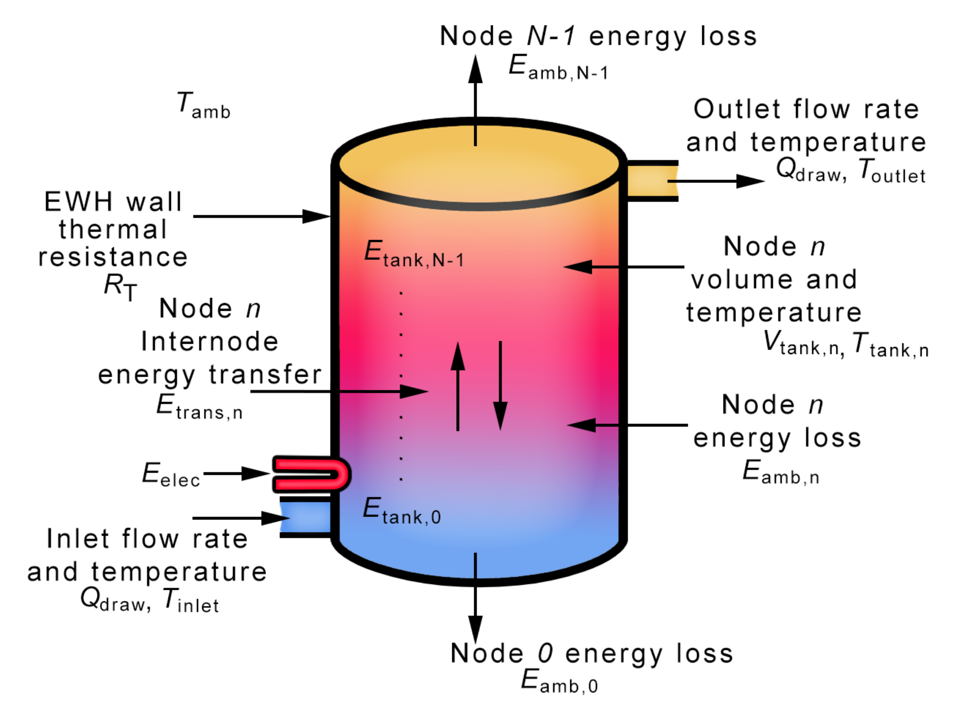
3.2. EWH Simulation Model

The simulation results were produced using a vertically orientated multi-node EWH model to simulate the energy flow inside the tank and determine the overall energy consumption. The EWH was modelled as a stack of N thermal layers. Each layer has a uniform temperature and a constant volume, and stratification occurs with the adjacent layers. Figure 1 shows a diagram of the multi-node EWH, and the colour gradient represents the temperature profile that is mimicked by the N nodes.

When water is drawn from the tank, the water leaves through the outlet pipe at the temperature of the uppermost node $N-1$. This water is replaced with cold water entering through the inlet pipe at the lowermost node 0. A heating element is situated at the bottom of the tank and supplies electrical energy to node 0. Thermal energy is lost to the surrounding environment due to standing losses. The rate of standing losses for each node is determined by the thermal resistance of the tank wall that encapsulates each node, $R_{\mathrm{T}}$, and the temperature difference between the ambient temperature, $T_{\mathrm{amb}}$, and the temperature of the water in node n. Further information describing the thermodynamics of this model can be found in [31].

3.3. Heating Control Strategies

This section describes the three types of heating control strategies that are used in this study.

The baselinestrategy is referred to as thermostat control (TC) and is used when no other heating control strategy is specified. For this strategy, the thermostat is “always-on,” and the temperature of the water inside the tank is maintained at the set-point temperature. Although this is the method that is traditionally used in households, it wastes a high amount of energy because the tank remains hot for long periods, even when the EWH is not used.

The other two strategies use optimal control (OC), where the optimal switching sequence of the heating element is predetermined for the known hot water usage profile. Where the previous strategy is vastly inefficient, OC minimises the electrical energy required by the heating element to satisfy the hot water profile of the household such that the user does not experience water temperatures below 40 ${}^{°}\mathrm{C}$ during usage. With these strategies, heating only occurs right before each water usage, and the time required for the heating element to turn on is predetermined so that the desired outlet temperature is reached just before the start of the usage. The optimisation algorithm that obtains the optimal heating plan is elaborated on in [31].

The first optimal control strategy is temperature matching (TM), which implies that the temperature at the start of each instance of water usage must be exactly matched to that of the identical water usage instance with TC. This ensures that the water temperature experienced by the user is not negatively affected.

The second optimal strategy is energy matching with Legionella prevention (EML). This implies that energy used during each water usage must be exactly matched to that of the identical water usage that occurred at the same time of the day using an EWH controlled with TC. This ensures that the thermal energy delivered to the user is not negatively affected, despite the lower outlet water temperature. Additionally, the tank is sufficiently heated to 60 ${}^{°}\mathrm{C}$ for 11 min during every day to prevent the growth of Legionella [30].

3.4. Simulation Setup

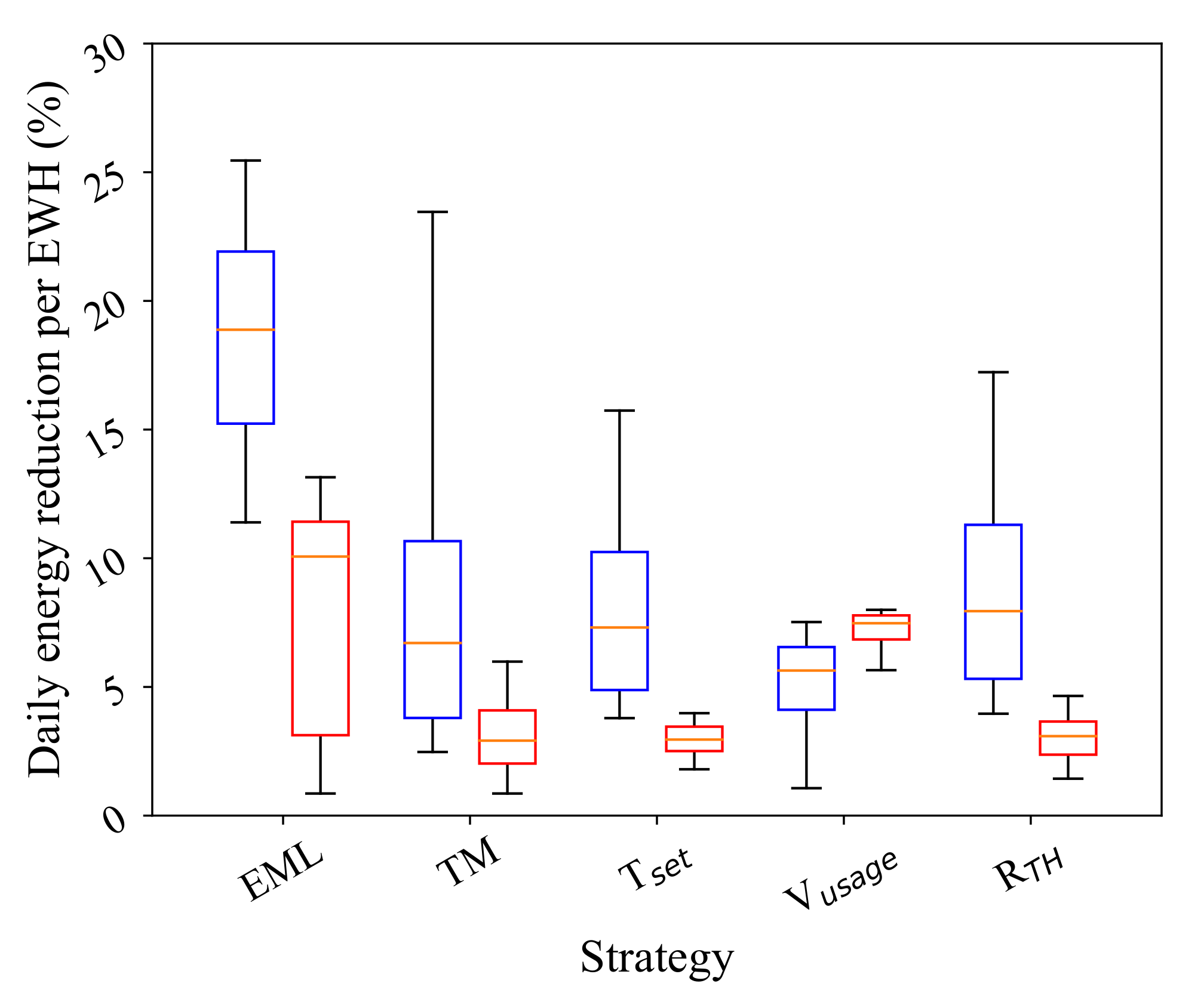
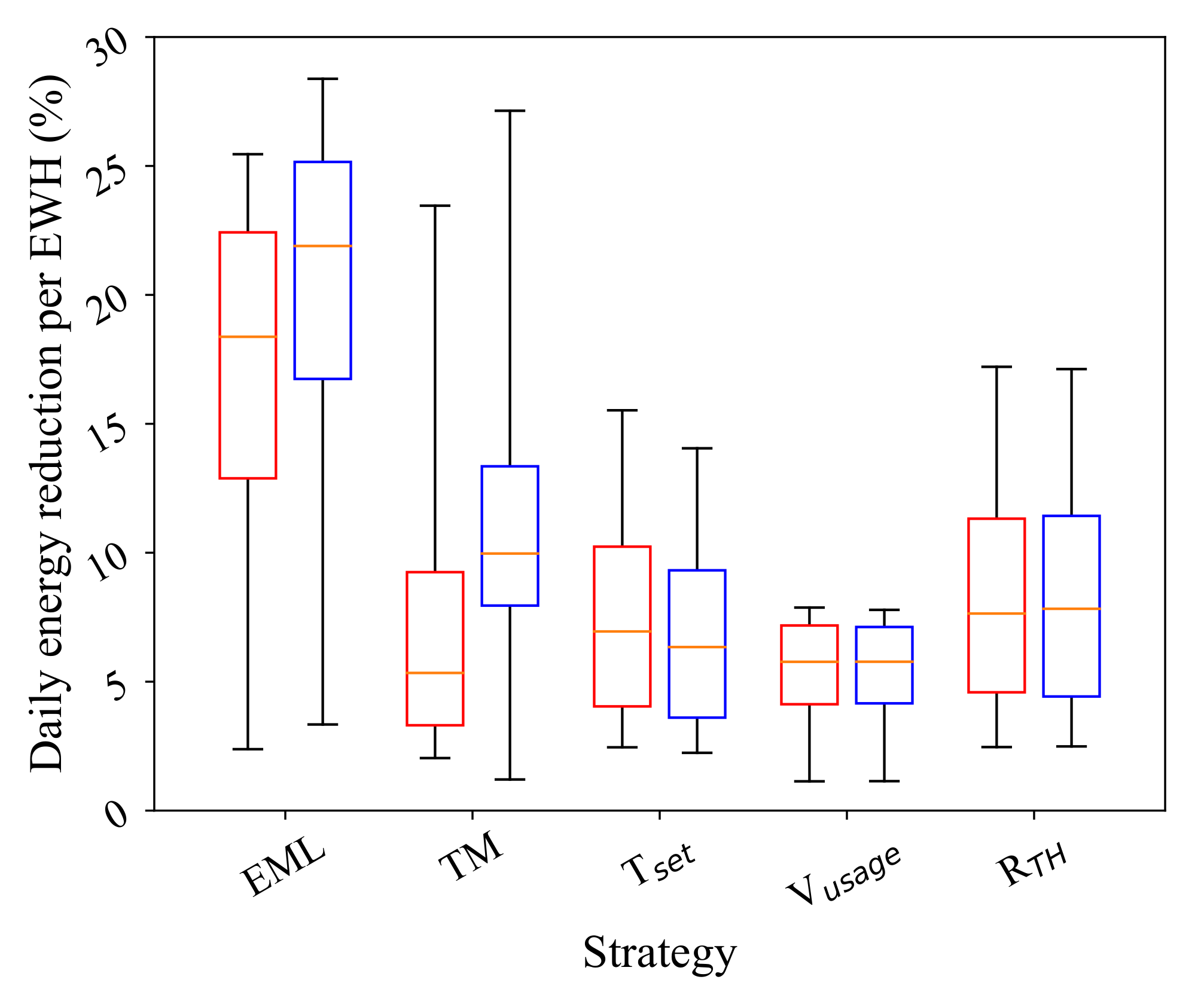
The baseline energy consumption was obtained using the TC heating control strategy on a 4-node EWH model. The baseline EWH parameters are presented in

Table 1. EWH parameters used for the baseline energy consumption. Note: K is Kelvin.

Parameter	Description	Value
$P_{\mathrm{rated}}$	Power rating of heating element	3 kW
$T_{\mathrm{set}}$	Set-point temperature	68.5  ${}^{°}\mathrm{C}$
$T_{\mathrm{hyst}}$	Hysteresis	$\pm 1.5$${}^{°}\mathrm{C}$
$T_{\mathrm{amb}}$	Ambient temperature	20  ${}^{°}\mathrm{C}$
$T_{\mathrm{inlet}}$	Inlet water temperature	20  ${}^{°}\mathrm{C}$
$R_{\mathrm{TH}}$	Thermal resistance of EWH	0.4807 $\frac{\mathrm{K}·\mathrm{day}}{\mathrm{kWh}}$
$V_{\mathrm{tank}}$	Tank volume	150 L

. The energy savings were determined with the various strategies by modifying the parameters or changing the heating control strategy accordingly, simulating 77 EWHs for hot water usage profiles in all seasons and comparing the energy usage of each simulation to the baseline energy consumption.

We determined the energy savings when OC (for both TM and EML) is used on a 4-node EWH model for known water usage patterns. We also determined the energy savings achieved by adjusting the set-point temperature, the volume of water used, the tank size, and the thermal resistance by installing thermal blankets or pipe insulation (increasing the EWH thermal resistance by 18% and 6%, respectively [10,35]), and results are presented in

Table 2. Simulation results obtained by the various strategies for 77 EWHs.

Strategy	Value	Energy Losses (kWh/day)	Energy Used (kWh/day)	Total EWH Energy (kWh/day)	$\mathit{\eta }$ - Energy Efficiency (%)	$\mathbf{\Delta }$Energy Losses (kWh/day)	$\mathbf{\Delta }$Energy Used (kWh/day)	$\mathbf{\Delta }$Total EWH Energy (kWh/day)	$\mathbf{\Delta }$$\mathit{\eta }$ (Percentage Points)
Baseline	-	2.40	4.77	7.16	66.3	-	-	-	-
Optimal control (TM)	-	2.02	4.77	6.75	75.2	0.367	0.000	0.385	8.9
Optimal control (EML)	-	1.34	4.77	6.06	85.5	1.06	0.000	1.09	19.2
$T_{\mathrm{set}}$	55 ${}^{°}$C	1.73	4.74	6.48	73.1	0.666	0.000	0.666	6.83
	60 ${}^{°}$C	1.98	4.77	6.75	70.4	0.420	0.000	0.419	4.1
	70 ${}^{°}$C	2.47	4.76	7.24	65.6	−0.074	0.001	−0.073	−0.710
$T_{\mathrm{amb}}$	10 ${}^{°}$C	2.89	4.78	7.68	62.0	−0.495	0.003	−0.491	−4.25
	15 ${}^{°}$C	2.65	4.77	7.41	64.3	−0.248	0.003	−0.244	−1.96
$T_{\mathrm{inlet}}$	10 ${}^{°}$C	2.39	5.74	8.14	70.3	0.007	−0.952	−0.945	4.01
	15 ${}^{°}$C	2.40	5.26	7.66	68.5	0.003	−0.484	−0.480	2.19
$V_{\mathrm{usage}}$	−5%	2.40	4.53	6.93	65.2	−0.001	0.230	0.229	−1.10
	−10%	2.40	4.30	6.70	64.0	−0.003	0.459	0.457	−2.26
	−15%	2.40	4.06	6.46	62.5	−0.003	0.693	0.689	−3.78
	−20%	2.40	3.82	6.22	61.4	−0.004	0.927	0.923	−4.93
Thermal blanket	18%	2.04	4.77	6.81	69.9	0.363	−0.007	0.356	3.59
Pipe insulation	6%	2.26	4.77	7.03	67.8	0.135	−0.004	0.131	1.46
Thermal blanket + pipe insulation	24%	1.94	4.78	6.72	70.9	0.461	−0.008	0.452	4.63
Tank size	200 L	2.77	4.78	7.55	59.8	−0.371	0.004	−0.367	−6.47

. The ambient and water inlet temperature is also adjusted to evaluate their impact on the overall energy consumption.

When the set-point temperature is lowered in reality, the water usage behaviour of the user is expected to change in reaction to the lower outlet temperature. For this strategy, the user and water mixer were simulated to adjust the mixing of hot and cold water in reaction to the initial temperature experienced during water usage. This ensured that the energy usage will be equivalent to that obtained by the baseline strategy.

We expand further on our evaluation of energy savings for each strategy by determining the results when households are categorised by their water usage intensity. A household is classified as having a light or heavy water usage profile if the total volume of water used is below or above a usage threshold.

We evaluated the impact of seasonality on energy savings by simulating the households for summer and winter. For each season, we only performed simulations on hot water usage profiles that were recorded during the corresponding season. The ambient and inlet water temperatures were also modified for each season accordingly. Using real weather data obtained for the Western Cape, South Africa, these temperatures are assumed to be 20 ${}^{°}\mathrm{C}$ for summer and 15 ${}^{°}\mathrm{C}$ for winter [36] and are in line with those acquired in [22].

Lastly, we determine the parameters required to achieve the same average energy savings as the EML strategy.

4. Results

The results when implementing OC with the TM and EML heating control strategies, adjusting the set-point temperature, $T_{\mathrm{set}}$, reducing the volume of water used during usages, $V_{\mathrm{usage}}$, and increasing the thermal resistance of the tank and pipes, $R_{\mathrm{TH}}$, are summarised in Table 2 and discussed in this section.

Figure 2 shows box plots of the daily energy savings (%) for the various strategies. The results for $T_{\mathrm{set}}$ lowered the set point to 60 ${}^{°}\mathrm{C}$, $V_{\mathrm{usage}}$ reduced the volume of water usages by 10%, and $R_{\mathrm{TH}}$ installed thermal blankets and pipe insulation. The best median savings of 16.3% are achieved by using the EML optimal control strategy. Following this, the best median savings of 6.3% were achieved by installing thermal blankets and pipe insulation. The remaining median energy savings were 6.2% for $V_{\mathrm{usage}}$, 5.9% for $T_{\mathrm{set}}$, and 5.2% when using the TM optimal control strategy. The same energy savings achieved by EML could also be approximately obtained when the $T_{\mathrm{set}}$, $V_{\mathrm{usage}}$, and $R_{\mathrm{TH}}$ strategies were combined.

The variance in energy savings for each strategy is due to the dependence of that strategy on the characteristics of the household usage profile. Households that use less water will save more energy with strategies that reduce standing losses since a larger portion of the consumed energy contributes to standing losses. The variance in energy savings is significantly large with EML, where savings can range from 2% to 26%.

Figure 3 shows box plots of the daily energy savings. The results are classified into light (blue) and heavy (blue) water usage intensities. An EWH is classified as having a light usage intensity if it draws less than 4500 L of hot water over the month; otherwise, it is classified as having a heavy usage intensity.

The most significant change in energy savings was observed for EML with a median energy saving of 18.9% for light- and 10.1% for heavy-usage EWHs. Even though both of these savings were still higher than those of the light- and heavy-usage EWHs for TM, $T_{\mathrm{set}}$, $V_{\mathrm{usage}}$, and $R_{\mathrm{TH}}$, the degree of energy savings was strongly correlated to the EWH usage intensity. The only strategy to have higher energy savings for the heavy-usage EWHs was $V_{\mathrm{usage}}$. Since the reduction of water usage scales with the total volume of hot water drawn, it is expected that a heavier water usage profile would achieve higher savings. It can also be seen that the energy savings for heavy-usage EWHs have a notably lower variance for $T_{\mathrm{set}}$, $V_{\mathrm{usage}}$, and $R_{\mathrm{TH}}$.

Figure 4 shows box plots of the daily energy savings for summer (red) and winter (blue). The distribution of daily volume of hot water used by the 77 EWHs for summer and winter, where the distribution is represented as 25th, 50th, 75th, was 29.6, 63.1, 144.5 and 52.6, 123.8, 195.2, respectively.

Since the ambient and inlet water temperatures are also changed for summer and winter, the energy consumption obtained for each considered season was compared with a modified baseline energy consumption that was produced using the corresponding parameter adjustments. This ensures that the energy savings are accurate and fairly calculated. By comparing the results for EML, the median energy savings of 21.9% for winter is 3.5 percentage points higher than the 18.4% achieved for summer. A similar trend was also observed for TM. The reason for this, despite the heavier usage in winter, is that the energy consumption for winter was compared to the baseline heating control strategy for a lower ambient and inlet water temperature. This means that the standing losses and energy usage with the baseline strategy are higher, and more heating is required to ensure that the water temperature is maintained at the set point.

The energy savings are slightly lower in winter for $T_{\mathrm{set}}$, and almost identical in both seasons for $V_{\mathrm{usage}}$ and $R_{\mathrm{TH}}$.

Table 2 summarises the simulation results for all the strategies. The first and second column shows the strategy and adjusted parameter value. The following four columns show the median results of all the EWHs. The last four columns show the median energy savings of the results when compared to the baseline strategy. The total EWH energy (kWh/day) is a sum of the total energy losses (kWh/day) and total energy used (kWh/day).

The daily energy savings using the TM and EML heating control strategies were 0.385 kWh and 1.09 kWh. This confirms that EML performed remarkably better than TM. This resulted in the EML control strategy having an energy efficiency of 85.5%, 10 percentage points higher than TM.

The daily energy savings for lowering the set-point temperature to 55 ${}^{°}\mathrm{C}$ and 60 ${}^{°}\mathrm{C}$ was 0.666 kWh and 0.419 kWh.

Lowering the ambient temperature to 10 and 15 ${}^{°}\mathrm{C}$ increased the total daily energy consumption by 0.491 and 0.244 kWh. Lowering the inlet water temperature to 10 and 15 ${}^{°}\mathrm{C}$ increased the total daily energy consumption by 0.945 kWh and 0.480 kWh. This means that adjusting the inlet water temperature impacts the reduction in energy savings by about a factor of 2 more than adjusting the ambient temperature.

It can be seen that reducing the volume of water used for $V_{\mathrm{usage}}$ had negligible effects on the standing losses. Instead, a larger volume reduction resulted in less energy used, and up to 0.923 kWh can be saved daily if the user shortens their volume of hot water used or usage duration by 20%. Moreover, the reduction in usage energy resulted in an energy efficiency performing up to 4.93 percentage points worse than the baseline energy consumption.

A comparison of the results for increasing the thermal insulation by a thermal blanket and pipe insulation shows that the effect of installing a thermal blanket has more than double the impact as pipe insulation.

Increasing the size of the tank to 200 L showed an increase in the overall daily energy consumption by 0.367 kWh. This is caused by the increase in standing losses as a result of a larger tank surface area.

After obtaining the energy savings of each strategy, we then determined what parameters would be required such that the median energy savings would match the 16.3% achieved by EML:

• For $T_{\mathrm{set}}$, the set-point must be set to 45.5 ${}^{°}\mathrm{C}$.
• For $V_{\mathrm{usage}}$, the volume of water used must be reduced by 25.4%.
• For $R_{\mathrm{TH}}$, the thermal resistance of the EWH must increase by 96%.

When comparing the median daily energy savings using the various methods in Figure 2, the energy savings of 16.3% for optimal control with EML were significantly higher than those achieved by the other methods where the median energy savings ranged from 5.2% to 6.3%.

Furthermore, Figure 3 and Figure 4 show that looking at the overall daily energy savings does not reflect the savings that can be expected by the user. The extent of energy savings depends on the household’s level of water usage, where median energy savings can vary from 10.1% for heavy usage to 18.9% for light usage using EML, and on seasonality, where median energy savings can vary from 18.4% for summer to 21.9% for winter using EML.

The aspects that are controllable by the user generally have the most positive impact on energy savings. Whereas the total EWH energy using the baseline strategy used a mean of 7.16 kWh/day over all the EWHs, the achieved energy reductions were 0.385 kWh/day with TM, 1.09 kWh/day with EML, 0.666 kWh/day when lowering the set-point temperature to 55 ${}^{°}\mathrm{C}$, and 0.923 kWh/day when reducing the total volume of hot water used by 20%. The environmental aspects that influenced the ambient and inlet water temperature showed a total EWH energy increase of 0.491 kWh/day and 0.945 kWh/day when the ambient and inlet water temperatures dropped from 20 to 10 ${}^{°}\mathrm{C}$. Changing the physical aspects of the EWH showed total EWH energy reductions of 0.356 kWh/day when installing a thermal blanket, 0.131 kWh/day when installing pipe insulation, and 0.452 kWh/day when installing a thermal blanket and pipe insulation, and the total EWH energy increased by 0.367 kWh/day when the tank size increased to 200 L.

The energy savings with EML can be achieved if the set-point temperature is lowered to 45.5 ${}^{°}\mathrm{C}$. This is a plausible solution provided that no heavy water usages occur. Since the outlet water temperature is only 5.5 ${}^{°}\mathrm{C}$ above the minimum temperature to satisfy the user, the risk of cold event occurrences is increased. The same energy savings are achieved if the user reduces their total volume of water use by 25.4%. This can also be realistically achieved if the user is willing to change their hot water usage habits. Lastly, the same energy savings can be achieved if the thermal resistance of the EWH is increased by 96% but is not realistically feasible.

5. Conclusions

In this paper, we determined how the best energy savings can be achieved for a residential household’s EWH. We evaluated the results of strategies that optimised the EWH heating schedule: lowering the set-point temperature, reducing the volume of hot water used, and installing additional thermal insulation.

The key findings of this research were that providing optimal control of the heating element with the EML strategy achieved the best median energy savings of 16.3%. However, the extent of savings depends on the household’s water usage, where the savings for light and heavy water usage profiles for EML were 18.9% and 10.1%. Seasonality also plays a role in energy savings, and the energy reductions for summer and winter differed by 3.5%. The impact of lowering the ambient and inlet water temperature to 10 ${}^{°}\mathrm{C}$ increased the total daily energy consumption by 0.491 and 0.945 kWh.

Furthermore, the various strategies can achieve the same savings as EML if the set-point temperature is lowered to 45.5 ${}^{°}\mathrm{C}$, lowering the volume of water used by 25.4% and increasing the thermal resistance of the EWH by 96%. In future work, this study can provide insight for the implementation of various methods to achieve EWH energy savings. A limitation of this study is that the optimal control planning is calculated with perfect foreknowledge of future water usage, and results will differ when forecasting is introduced. The simulations also did not use time-varying ambient and inlet water temperatures. Lastly, the water usage data was acquired from only South African households. However, this data has been proven to be significantly similar to that used in other international studies [37].

References

1. Tejero-Gómez, J.A.; Bayod-Rújula, A.A. Energy management system design oriented for energy cost optimization in electric water heaters. Energy Build. 2021, 243, 111012. [Google Scholar] [CrossRef]
2. Mathu, K. Cleaning South Africa’s Coal Supply Chain. J. Bus. Divers. 2017, 17. [Google Scholar] [CrossRef]
3. Jamie, M. Ramaphosa Announces Plan to Save Eskom and Stop Load-Shedding; MyBroadband 2021. Available online: https://mybroadband.co.za/news/energy/386264-ramaphosa-announces-plan-to-save-eskom-and-stop-load-shedding.html (accessed on 6 August 2021).
4. Rothausen, S.G.; Conway, D. Greenhouse-gas emissions from energy use in the water sector. Nat. Clim. Chang. 2011, 1, 210–219. [Google Scholar] [CrossRef]
5. Osório, G.J.; Shafie-khah, M.; Carvalho, G.C.; Catalão, J.P. Analysis Application of Controllable Load Appliances Management in a Smart Home. Energies 2019, 12, 3710. [Google Scholar] [CrossRef] [Green Version]
6. Salameh, W.; Faraj, J.; Harika, E.; Murr, R.; Khaled, M. On the Optimization of Electrical Water Heaters: Modelling Simulations and Experimentation. Energies 2021, 14, 3912. [Google Scholar] [CrossRef]
7. Ritchie, M.J.; Engelbrecht, J.A.; Booysen, M.J. Practically-achievable energy savings with the optimal control of stratified water heaters with predicted usage. Energies 2021, 14, 1963. [Google Scholar] [CrossRef]
8. Haase, P.; Thomas, B. Test and optimization of a control algorithm for demand-oriented operation of CHP units using hardware-in-the-loop. Appl. Energy 2021, 294, 116974. [Google Scholar] [CrossRef]
9. Hohne, P.; Kusakana, K.; Numbi, B. A review of water heating technologies: An application to the South African context. Energy Rep. 2019, 5, 1–19. [Google Scholar] [CrossRef]
10. Dutkiewicz, R.K. Energy for Hot Water in the Domestic Sector. In Proceedings of Domestic Use of Electrical Energy Conference; Energy Research Institute: Cape Town, South Africa, 1990; pp. 6–11. [Google Scholar]
11. Harris, A.; Kilfoil, M.; Uken, E. Domestic Energy Savings with Geyser Blankets; Cape Peninsula University of Technology, Cape Town, South Africa. 2007. Available online: http://digitalknowledge.cput.ac.za/bitstream/11189/3457/1/Harris%2C_Domestic_2007.pdf (accessed on 6 August 2021).
12. Diao, R.; Lu, S.; Elizondo, M.; Mayhorn, E.; Zhang, Y.; Samaan, N. Electric water heater modeling and control strategies for demand response. In Proceedings of the 2012 IEEE Power and Energy Society General Meeting, San Diego, CA, USA, 22–26 July 2012; pp. 1–8. [Google Scholar] [CrossRef]
13. Kepplinger, P.; Huber, G.; Petrasch, J. Autonomous optimal control for demand side management with resistive domestic hot water heaters using linear optimization. Energy Build. 2015, 100, 50–55. [Google Scholar] [CrossRef]
14. Nel, P.; Booysen, M.J.; Van der Merwe, B. Saving on household electric water heating: What works best and by how much? In Proceedings of the 2017 IEEE Innovative Smart Grid Technologies-Asia (ISGT-Asia), Auckland, New Zealand, 4–7 December 2017; pp. 1–6. [Google Scholar] [CrossRef] [Green Version]
15. Fuentes, E.; Arce, L.; Salom, J. A review of domestic hot water consumption profiles for application in systems and buildings energy performance analysis. Renew. Sustain. Energy Rev. 2018, 81, 1530–1547. [Google Scholar] [CrossRef]
16. Matos, C.; Bentes, I.; Pereira, S.; Faria, D.; Briga-Sa, A. Energy consumption, CO2 emissions and costs related to baths water consumption depending on the temperature and the use of flow reducing valves. Sci. Total Environ. 2019, 646, 280–289. [Google Scholar] [CrossRef] [PubMed]
17. Pereira, T.C.; Lopes, R.A.; Martins, J. Exploring the energy flexibility of electric water heaters. Energies 2019, 13, 46. [Google Scholar] [CrossRef] [Green Version]
18. Gato, S.; Jayasuriya, N.; Roberts, P. Forecasting residential water demand: Case study. J. Water Resour. Plan. Manag. 2007, 133, 309–319. [Google Scholar] [CrossRef]
19. Heidari, A.; Olsen, N.; Mermod, P.; Alahi, A.; Khovalyg, D. Adaptive hot water production based on Supervised Learning. Sustain. Cities Soc. 2021, 66, 102625. [Google Scholar] [CrossRef]
20. Yildiz, B.; Bilbao, J.I.; Roberts, M.; Heslop, S.; Dore, J.; Bruce, A.; MacGill, I.; Egan, R.J.; Sproul, A.B. Analysis of electricity consumption and thermal storage of domestic electric water heating systems to utilize excess PV generation. Energy 2021, 235, 121325. [Google Scholar] [CrossRef]
21. Jacobs, H.; Botha, B.; Blokker, M. Household Hot Water Temperature—An Analysis at End-Use Level. In Proceedings of the WDSA/CCWI Joint Conference Proceedings, Kingston, ON, Canada, 23–25 July 2018; Volume 1. [Google Scholar]
22. Agudelo-Vera, C.; Avvedimento, S.; Boxall, J.; Creaco, E.; de Kater, H.; Di Nardo, A.; Djukic, A.; Douterelo, I.; Fish, K.E.; Iglesias Rey, P.L.; et al. Drinking water temperature around the globe: Understanding, policies, challenges and opportunities. Water 2020, 12, 1049. [Google Scholar] [CrossRef] [Green Version]
23. Iglesias, F.; Palensky, P. Profile-based control for central domestic hot water distribution. IEEE Trans. Ind. Inform. 2013, 10, 697–705. [Google Scholar] [CrossRef]
24. Zhou, S.; McMahon, T.; Walton, A.; Lewis, J. Forecasting operational demand for an urban water supply zone. J. Hydrol. 2002, 259, 189–202. [Google Scholar] [CrossRef]
25. Gerin, O.; Bleys, B.; De Cuyper, K. Seasonal variation of hot and cold water consumption in apartment buildings. In Proceedings of the CIB W062, 40th International Symposium on Water Supply and Drainage for Building, Sao Paulo, Brazil, 8–10 September 2014; pp. 1–9. [Google Scholar]
26. Roux, M.; Booysen, M.J. Use of smart grid technology to compare regions and days of the week in household water heating. In Proceedings of the 2017 International Conference on the Domestic Use of Energy (DUE), Cape Town, South Africa, 4–5 April 2017; pp. 276–283. [Google Scholar] [CrossRef] [Green Version]
27. Booysen, M.J.; Visser, M.; Burger, R. Temporal case study of household behavioural response to Cape Town’s “Day Zero” using smart meter data. Water Res. 2019, 149, 414–420. [Google Scholar] [CrossRef] [Green Version]
28. Armstrong, P.M.; Uapipatanakul, M.; Thompson, I.; Ager, D.; McCulloch, M. Thermal and sanitary performance of domestic hot water cylinders: Conflicting requirements. Appl. Energy 2014, 171–179. [Google Scholar] [CrossRef]
29. Stone, W.; Louw, T.M.; Gakingo, G.K.; Nieuwoudt, M.J.; Booysen, M.J. A potential source of undiagnosed Legionellosis: Legionella growth in domestic water heating systems in South Africa. Energy Sustain. Dev. 2019, 130–138. [Google Scholar] [CrossRef] [Green Version]
30. Stout, J.E.; Best, M.G.; Yu, V.L. Susceptibility of members of the family Legionellaceae to thermal stress: Implications for heat eradication methods in water distribution systems. Appl. Environ. Microbiol. 1986, 52, 396–399. [Google Scholar] [CrossRef] [PubMed] [Green Version]
31. Ritchie, M.J.; Engelbrecht, J.; Booysen, M.J. Impact of node count on energy-optimal control of stratified vertical water heaters in smart grid applications. Prepr. Curr. Under Rev. 2021. [Google Scholar] [CrossRef]
32. Fikru, M.G.; Gautier, L. The impact of weather variation on energy consumption in residential houses. Appl. Energy 2015, 144, 19–30. [Google Scholar] [CrossRef]
33. Booysen, M.J.; Engelbrecht, J.; Ritchie, M.J.; Apperley, M.; Cloete, A.H. How much energy can optimal control of domestic water heating save? Energy Sustain. Dev. 2019, 51, 73–85. [Google Scholar] [CrossRef] [Green Version]
34. Geasy-A Smart Geasy Controller by BridgIoT. Available online: https://www.bridgiot.co.za/solutions/geasy-2/ (accessed on 17 September 2019).
35. Bosman, I.; Grobler, L.; Dalgleish, A. Determination of the impact on the standing losses of installing blankets to electric hot water heaters in South Africa. J. Energy South. Afr. 2006, 17, 57–64. [Google Scholar]
36. Climate-data.org-Cape Town Climate. Available online: https://en.climate-data.org/africa/south-africa/western-cape/cape-town-788/ (accessed on 6 August 2021).
37. Ritchie, M.; Engelbrecht, J.; Booysen, M. A probabilistic hot water usage model and simulator for use in residential energy management. Energy Build. 2021, 235, 110727. [Google Scholar] [CrossRef]
Figure 1. Energy flow, thermal resistance, flow rate, temperature, and volume in a multi-node EWH.
Energies 14 04859 g001
Figure 2. Box plot showing the distribution of the daily reduction in energy consumed (as a percentage) by each EWH compared to that produced by the baseline energy consumption for T set (set to 60 ° C ), V usage (10% reduction), and R TH (thermal blankets and pipe insulation).
Energies 14 04859 g002
Figure 3. Box plot showing the distribution of the daily reduction in energy consumed (as a percentage) by light- (blue) and heavy-usage (red) EWHs compared to that produced by the baseline energy consumption for T set (set to 60 ° C ), V usage (10% reduction), and R TH (thermal blankets and pipe insulation).
Energies 14 04859 g003
Figure 4. Box plot showing the distribution of the daily reduction in energy consumed (as a percentage) for summer (red) and winter (blue) by each EWH compared to that produced by the baseline energy consumption for T set (set to 60 ° C ), V usage (10% reduction), and R TH (thermal blankets and pipe insulation).
Energies 14 04859 g004