Study on Image Correction and Optimization of Mounting Positions of Dual Cameras for Vehicle Test

Abstract

Among surrounding information-gathering devices, cameras are the most accessible and widely used in autonomous vehicles. In particular, stereo cameras are employed in academic as well as practical applications. In this study, commonly used webcams are mounted on a vehicle in a dual-camera configuration and used to perform lane detection based on image correction. The height, baseline, and angle were considered as variables for optimizing the mounting positions of the cameras. Then, a theoretical equation was proposed for the measurement of the distance to the object, and it was validated via vehicle tests. The optimal height, baseline, and angle of the mounting position of the dual camera configuration were identified to be 40 cm, 30 cm, and 12°, respectively. These values were utilized to compare the performances of vehicles in stationary and driving states on straight and curved roads, as obtained by vehicle tests and theoretical calculations. The comparison revealed the maximum error rates in the stationary and driving states on a straight road to be 3.54% and 5.35%, respectively, and those on a curved road to be 9.13% and 9.40%, respectively. It was determined that the proposed method is reliable because the error rates were less than 10%.

1. Introduction

Driving automation, as defined by the Society of Automotive Engineers (SAE), is the internationally accepted standard. SAE provides taxonomy with detailed definitions for six levels of driving automation. These range from no driving automation (Level 0) to full driving automation (Level 5) [1]. Mass-produced vehicles have recently begun to be generally equipped with Level 2 autonomous driving technology. This technology provides drivers with partial driving automation and is called advanced driver assistance systems (ADAS). Among the examples of ADAS, adaptive cruise control (ACC) and lane-keeping assist system (LKAS) are Level 1 technologies, and highway driving assist (HDA) is a Level 2 technology.

The primary goal of autonomous driving technology is to respond proactively to unanticipated scenarios, such as traffic accidents and construction sites. This requires rapid and effective identification of the environment surrounding the vehicle. To achieve this, various sensors, such as light detection and ranging (LiDAR) and radar sensors, and cameras are used for detection [2]. Among these, cameras capture images containing a large quantity of information. This information enables object detection, traffic information collection, lane detection, among other tasks. Furthermore, cameras are more readily accessible compared to other sensors. Therefore, several studies have been conducted on the camera-based collection of environmental information and its processing.

With regard to the correction of camera images, Lee et al. [3] proposed a method to correct the radial distortion caused by camera lenses. In addition, Detchev et al. [4] proposed a method for simultaneously estimating the internal and relative direction parameters for calibrating measurement systems comprising multiple cameras.

With regard to camera-based lane detection, Kim et al. [5] proposed an algorithm to improve nocturnal lane detectability based on image brightness correction and the lane angle. In addition, Kim et al. [6] performed real-time lane detection using the lane path obtained based on the lane gradient and width information in conjunction with the previous frame. Choi et al. [7] proposed and validated a novel lane detection algorithm (namely random sample consensus (RANSAC) algorithm) by applying conventional lane detection algorithms. Kalms et al. [8] used the Viola-Jones object detection method to design and implement an algorithm for lane detection and autonomous driving. Wang et al. [9] achieved lane detection through pre-processing images and utilized the features extracted from the image pixel coordinates to detect lane departure using a stacked sparse autoencoder (SSAE). Andrade et al. [10] recommended a novel three-stage strategy for lane detection and tracking, comprising image correction and region of interest (ROI) set-up, edge detection.

With regard to monocular camera-based distance measurement, Bae et al. [11] proposed a method to measure the distance to the vehicle in front using the relationship between the lane and the geometry of the camera and the vehicle. A method suggested by Park et al. [12] involved measuring distances by training the distance classifier using the distance information obtained from LiDAR sensors in conjunction with the width and height of the bounding box corresponding to the detected object. Huang et al. [13] proposed a method to estimate inter-vehicle distances based on monocular camera images captured by cameras installed within a vehicle by combining the vehicular attitude angle information with the segmentation information. Moreover, Zhe et al. [14] constructed an area-distance geometric model based on the camera projection principle. They leveraged the advantages of 3D detection to combine the 3D detection of vehicles with the distance measurement model, proposing a robust inter-vehicle distance measurement method based on a monocular camera installed within a vehicle. Bongharriou et al. [15] combined vanishing point extraction, lane detection, and vehicle detection based on actual images and proposed a method to estimate distances between cameras and vehicles in front by correcting camera images.

Object detection and distance measurements using stereo cameras have also been researched extensively. Kim [16] proposed an algorithm to estimate vehicular driving lanes by generating 3D trajectories based on the coordinates of detected traffic signs, and Seo [17] proposed an improved distance measurement method using a disparity map. A method proposed by Kim et al. [18] comprises measuring distances by correcting image brightness and estimating central points of objects using two webcams. Furthermore, Song et al. [19] proposed a forward collision distance measurement method by combining a Hough space lane detection model with stereo matching. Additionally, Sie et al. [20] proposed an algorithm for real-time lane and vehicle detection and measurement of distances to vehicles in the driving lane by combining a portable embedded system with a dual-camera vision system. A method involving efficient pose estimation of on-board cameras using 3D point sets obtained from stereo cameras, and the ground surface was proposed by Sappa et al. [21]. Yang et al. [22] proposed a stereo vision-based system that detects vehicle license plates and calculates their 3D position in each frame for vehicular speed measurement. Zaarane et al. [23] proposed an inter-vehicle distance measurement system based on image processing utilizing a stereo camera by considering the position of vehicles in both the cameras and certain geometric angles. Cafiso et al. [24] proposed a system based on in-vehicle stereo vision and the global positioning system (GPS) to detect and assess collisions between vehicles and pedestrians. Wang et al. [25] proposed real-time object detection and depth estimation based on Deep Convolutional Neural Networks (DCNNs). Lin et al. [26] proposed a vision-based driver assistance system.

Several extensive studies have been conducted on the correction of camera images, road lane detection, and distance measurement. However, few studies have been conducted to optimize camera mounting positions and measure distances to objects in front of a vehicle. This gap is addressed in the present study by using testing and evaluation methods based on dual-camera-based image correction and lane detection. In this study, only theoretical concepts used in experiments are described in the computer vision phase for lane detection and the image distortion correction phase. In addition, focal length correction is performed after image distortion correction to reduce the effect of the change in detection distance caused by image distortion correction. Moreover, it investigates the three main variables related to the dual-camera installation. The experimental results according to installation height, camera baseline, and angle of inclination are presented. The parameters according to the camera’s rotation axis are set as roll, pitch, and pan. The pitch is the installation angle of the camera, and the parallel stereo camera method applied in this study does not consider roll and pan. In addition, the parameters such as angle-of-view and focal length of the camera are excluded from the analysis because the two cameras constituting the dual-camera configuration had the same specifications. The actual test was conducted on the three presented variables to determine the optimal position of the dual camera. The three variables were tested for three values, respectively. Based on the obtained optimal value, the actual test was conducted on the theoretical equation. This study proceeds as follows.

• Introduction of the lane detection algorithm.
• Input image distortion correction, stereo rectification, and focal length correction.
• Experimental evaluation of algorithm precision according to three variables for optimal dual-camera positioning.
• Proposal of equations for calculating the distance between the vehicle and objects in front of it in straight and curved roads for test evaluation.
• Applicability evaluation through real vehicle tests using the optimal camera position determined in step 3 and the distance calculation equation proposed in step 4.

2. Theoretical Background for Dual Camera-Based Image Correction and the Proposed Method of Distance Measurement

2.1. Road Lane Detection Method

2.1.1. Theoretical Background for Lane Detection

The ROI in a camera-captured image is the region containing the information relevant to the task at hand. As the range of the scenery captured by a camera affixed within a vehicle remains constant, the ROI in particular images must be obtained by removing the corresponding irrelevant regions.

Cameras usually capture images in the red, green, and blue (RGB) format, which comprises three channels. Grayscale conversion of such images produces monochromatic images, which comprise a single channel. As images converted via this method retain only brightness information, the amount of data to be processed is reduced by two-thirds, increasing the computational speed.

The canny edge detector is an edge detection algorithm that utilizes successive steps such as noise reduction, determination of the intensity gradient of the image, non-maximum suppression, and hysteresis thresholding [27]. Owing to its multi-step mechanism, it performs better than the methods that use differential operators (e.g., the Sobel mask).

The Hough transform is a method for transforming components in the Cartesian coordinate system to those in the parameter space [28]. Straight lines and points on the Cartesian coordinate system are represented by points and straight lines, respectively, in the parameter space. Thus, points of intersection between straight lines in the parameter space can be used to search for straight lines passing through a given set of points in the Cartesian coordinate system.

The hue, saturation, value (HSV) format is a color model that represents an image in terms of hue, saturation, and value. It is particularly effective for the facile expression of desired colors because its operational template agrees with the human mode of color recognition.

Perspective transform facilitates the modeling of homography using a 3 × 3 transformation matrix. The perspective of any image can be removed via a geometric processing method by relocating the pixels of the image.

The sliding window method uses a sub-level array of a certain size called a window and reduces the computational load for calculating the elements in each window in the entire array by reusing (rather than discarding) redundant elements.

The curve fitting method involves fitting a function to a given curve representing the input data. A polynomial function is most commonly used for this purpose. Furthermore, the input data can be approximated using a quadratic function by employing the least-squares approximation method.

2.1.2. Lane Detection Algorithm

Figure 1 depicts the algorithm used in this study for lane detection. It utilizes OpenCV, an open-source computer vision library, for image processing. After performing the lane detection algorithm, the detected lane information is used to calculate the distance to the object in front of the vehicle.

Figure 2a presents an input image captured by the fixed left camera. When the ROI corresponds to 20–50% of the image height and the resolution of the image is 1920 × 1080, it configures within a rectangular area having the following coordinate points as vertices: (0, 216), (1920, 216), (1920, 540), and (0, 540).

Figure 2c depicts the image obtained from the previous one via grayscale conversion. The single-channel image was generated by averaging the pixel values corresponding to the R, G, and B channels.

Figure 2d depicts the result of edge detection. A Gaussian filter was used to remove the noise, and the Canny edge detector was used to generate this edge-detected image. Then straight lines corresponding to the lane marks were obtained, as depicted in Figure 2e. The Hough transform was used to detect the edge components in the edge-detected image. Subsequently, straight lines corresponding to gradients with magnitudes of at most 5° were removed, resulting in the elimination of horizontal and vertical lines that were unlikely to correspond to the lane.

The yellow pixels were extracted from Figure 2b, and the result is depicted in Figure 2f. Following the conversion of the image from the RGB format to the HSV format, a yellow color range was selected. When the ranges of the hue channel, saturation channel, and value channel were normalized to the interval 0–1, the yellow pixels corresponded to values between 0–0.1, 0.9–1, and 0.12–1 for hue and saturation channels. One-third of the mean brightness of the image was used for the value channel. When the value of the pixel was within the range that was set, the value was set to 255; otherwise, it was set to zero.

Figure 2g depicts a combination of the image obtained by extracting straight lines to identify pixels corresponding to the lane candidates and that obtained by extracting the color. A combination was obtained by assigning weights of 0.8 and 0.2 to the images in Figure 2c,d, respectively.

Further, the lane candidates were obtained using the sliding window method after removing the perspective from the image presented in Figure 2g, and the output is depicted in Figure 2h. The image was captured in advance such that the optical axis of the camera was parallel to the road when the vehicle was located in the center of the straight road. The image can be warped so that the left and right lanes on a straight road are parallel. The coordinates (765, 246), (1240, 246), (1910, 426), and (5, 516) of the four points on the set of lanes visible within the ROI were relocated to the points (300, 648), (300, 0), (780, 0), and (780, 648) in the warped image to align these along straight lines. A square window comprising 54 pixels was selected, with a width and height that were one-twentieth and one-sixth, respectively, of those of the image. The window with the largest pixel sum was then identified via the sliding window method.

Subsequently, a lane curve was generated by fitting a quadratic curve to the pixels of the lane candidate, as depicted in Figure 2i. The quadratic curve fitting is performed using the least-squares method, and the positions of the pixels of the lane candidate are indicated by the six windows on the left and right lane marks in Figure 2h.

Finally, lane detection based on the input image was completed. The final result, obtained by applying the lane curve to the input image via perspective transform, is depicted in Figure 2j.

2.2. Method for Calibrating Distance Measurement

2.2.1. Image Distortion Correction

Images captured by cameras exhibit radial distortions due to the refractive indices of convex lenses and tangential distortions due to the horizontal leveling problem inherent to the manufacturing process of lenses and image sensors. Circular distortions induced by radial distortion at the edge of the image and elliptical distortions induced by the tangential distortion require correction. The values of pixels in the distorted image can be used as the values of the corresponding pixels in the corrected image by distorting the coordinates of each pixel in the image [29].

In this study, OpenCV’s built-in functions for checkerboard pattern identification, corner point identification, and camera calibration were adopted for image processing. To correct the input image, a 6 × 4 checkerboard image was captured using the camera, its corner points were identified, and the camera matrix and distortion coefficients were calculated based on the points obtained. Figure 3a depicts the identification of the corner points in the original image and Figure 3b depicts the screen after the removal of distortion.

2.2.2. Image Rectification

Parallel stereo camera configuration is the method that involves utilizing two cameras whose optical axes are parallel. It is particularly suitable for image processing because of the absence of vertical disparity [30]. In contrast, actual photographs require image rectification to correct the vertical disparity originating from the installation or internal parameters of cameras. This method corrects for an arbitrary object in the left and right images obtained with dual cameras to obtain equal coordinates for the height of images.

In this study, OpenCV’s built-in stereo calibration and stereo rectification functions were adopted for image processing. In addition, the checkerboard image utilized during the removal of the image distortion was used to identify the checkerboard pattern and its corner points and calibrate the dual cameras (Figure 4a). As depicted in Figure 4b, the internal parameters, rotation matrix of the dual-camera configuration, and projection matrix on the rectified coordinate system can be obtained based on a pair of checkerboard images captured using the dual cameras.

2.2.3. Focal Length Correction

Dual cameras were installed collinearly such that the optical axes of the two cameras are parallel. Furthermore, the lenses were positioned at identical heights above the ground. The 3D coordinates of any object were calculated relative to the camera positions, based on the geometry and triangulation of the cameras depicted in Figure 5. It can be described as follows:

$$\begin{array}{c}\mathrm{Z}=\frac{fb}{d}\\ \mathrm{X}=\frac{Z\left(xl+xr\right)}{2f}\\ \mathrm{Y}=\frac{Z\left(yl+yr\right)}{2f}\end{array}$$

(1)

where:

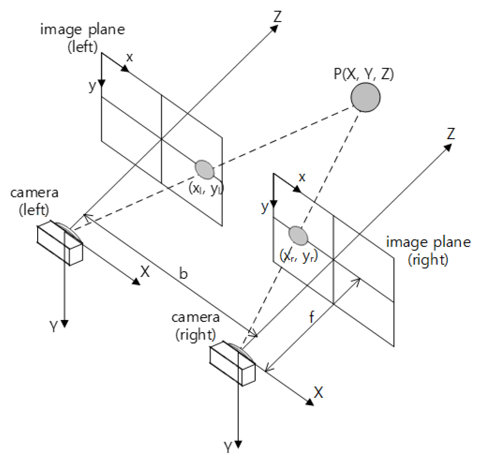
• $\mathrm{XYZ}$—the coordinates of the object; the local coordinate system with their origins at the center of dual cameras.
• $f$—focal length.
• $b$—baseline.
• $d$—disparity.
• $xl,yl$—the coordinates of the object in the left camera image plane.
• $xr,yr$—the coordinates of the object in the right camera image plane.

The focal length is an essential parameter in the calculation of the Z-coordinate. However, a problem with the use of inexpensive webcams is that some manufacturers do not provide details such as focal length. Further errors originating from image correction necessitate an accurate estimation of the focal length.

This can be achieved by employing curve-fitting based on actual data. Based on the relationship between distance and disparity, where $Z_a$ is calculated from the equation:

$$Z_a=\mathsf{\alpha }\frac{b}{d}+\beta$$

(2)

where:

• $\mathrm{XYZ}$—the coordinates of the object in the universal Cartesian coordinate system.
• $Z_a$—distance to the object.
• $\mathsf{\alpha }$,$\beta$—the coefficients obtained via the focal length correction.

During testing, images of objects installed at intervals of 0.5 m over the range of 1–5 m were captured. In addition, the differences between the X-coordinates of each object captured by the two cameras were recorded. Then, $\mathsf{\alpha }$ and $\beta$ were evaluated by fitting the curve described by the differences calculated via the least square method.

3. Optimization of the Mounting Positions of Dual Cameras

3.1. Configurations of Test Variables

3.1.1. Mounting Heights of Cameras

In the proposed equation, the distance is measured relative to the ground. It is evident that the mounting height of the cameras is inversely proportional to the fraction of the ground captured in the image. Therefore, the mounting height of the cameras wields a significant influence in the determination of the region captured in the image.

Heights of 30 cm, 40 cm, and 50 cm were considered. In the case of regular passenger cars, 30 cm was selected as the minimum value because their bumpers are at least 30 cm above the ground level. The maximum value was set to 50 cm because larger heights made it difficult to capture the ground within 1 m. Figure 6 depicts the input images corresponding to heights of 30 cm, 40 cm, and 50 cm where a baseline of cameras is 30 cm, and an angle of inclination of mounted cameras is 12°.

3.1.2. Baseline of Cameras

Equation (1) is based on the geometry and triangulation of the cameras. Therefore, the baseline between the cameras significantly affects the measurement of distance.

Baselines of 10 cm, 20 cm, and 30 cm were considered in this study. First, 10 cm was selected as the minimum value because it was the smallest feasible baseline. Then, the baseline was increased three times at intervals of 10 cm to examine its influence. Figure 7 depicts the input images corresponding to baselines of 10 cm, 20 cm, and 30 cm, where the mounting heights of the cameras are 40 cm, and the angle of inclination of the mounted cameras is 12°.

3.1.3. Angle of Inclination of Mounted Cameras

The installation of cameras parallel to the ground reduces the vertical range and hinders close-range supervision of the ground. Therefore, it is essential to utilize an optimal angle of inclination during the installation of cameras.

Angles of 3°, 7°, and 12° were considered as feasible angles of inclination. First, 3° was selected as the minimum value owing to the difficulty of capturing the ground within a radius of 1 m at smaller angles of inclination from a height of 50 cm. The proportion of the road captured in the image increased as the angle was increased. However, vehicular turbulence or the presence of ramps was observed to affect the inclusion of the upper part of the road in the images. Further, 12° was selected as the maximum angle of inclination as it yielded images with the road accounted for 20–80% of the vertical range. Figure 8 depicts input images corresponding to angles of inclination of 3°, 7°, and 12°, where the mounting heights of the cameras are 40 cm and the baseline of the cameras is 30 cm.

3.2. Test Results for Optimization of Mounting Positions

During testing, dual cameras were mounted on the vehicle, and objects were installed at distances ranging between 1 m–5 m at intervals of 0.5 m on an actual road. Then, the differences between the X-coordinates captured by the left and right cameras were computed and substituted into Equation (2) to verify the precision. The calculated results are presented in Figure 9, Figure 10 and Figure 11.

Figure 10 depicts the test results corresponding to a height of 40 cm. Figure 10a–c illustrates the variation in the degree of precision with respect to varying angles, corresponding to baselines of 10 cm, 20 cm, and 30 cm, respectively.

Figure 11 depicts the test results corresponding to a height of 50 cm. Figure 11a–c illustrates the variation in the degree of precision with respect to varying angles, corresponding to baselines of 10 cm, 20 cm, and 30 cm, respectively.

Table 1. Test results for optimization of mounting positions.

Height (cm)	Baseline (cm)	Angle (°)	Average Error Rate (%)	Maximum Error Rate (%)
30	10	3	13.28	48.62
		7	14.07	45.36
		12	14.15	53.04
	20	3	6.89	23.66
		7	9.64	27.3
		12	4.14	10.53
	30	3	10.34	35.83
		7	9.5	33.35
		12	8.34	33.99
40	10	3	5.55	13.77
		7	7.84	15.38
		12	8.18	26.9
	20	3	4.93	15.19
		7	2.38	6.17
		12	5.49	19.52
	30	3	3.34	13.9
		7	1.88	5.69
		12	0.86	2.15
50	10	3	10.62	32.49
		7	3.77	10.94
		12	8.19	27.67
	20	3	2.47	5.81
		7	2.45	5.84
		12	5.23	18.39
	30	3	2.15	4.65
		7	2.45	8.0
		12	1.32	2.34

summarizes the result of Figure 9, Figure 10 and Figure 11. It is evident from Figure 9, Figure 10 and Figure 11 that the error rate exhibited a decreasing tendency as the angle was increased. Meanwhile, it tended to decrease as the baseline was increased. Finally, the error rate decreased when the height was increased from 30 cm to 40 cm, and it increased when the height was increased to 50 cm.

Based on the aforementioned data, the best result was obtained corresponding to a height of 40 cm, a baseline of 30 cm, and an angle of inclination of 12°. In the next section, these values are used to validate the theoretical equation of distance measurement.

4. Proposed Theoretical Equation for Forward Distance Measurement

4.1. Measurement of the Distance to an Object in Front of the Vehicle on a Straight Road

The Z-coordinate of an object in front of the vehicle was obtained by using the coefficient α in Equation (2) (as evaluated via focal length correction) as the focal length and substituting it into Equation (1). However, during testing, the cameras were installed at an angle of inclination $\theta$, to capture the close-range ground. That is, the optical axes of the cameras and the ground were not parallel during testing.

The Z-coordinate of the object relative to the position of the camera can be calculated considering the angle $\theta$ in Equation (3):

$$\left[\begin{array}{c}{X}_g\\ Y_g\\ Z_g\end{array}\right]=\left[\begin{array}{ccc}1& 0& 0\\ 0& -\cos \theta & -\sin \theta \\ 0& -\sin \theta & \cos \theta \end{array}\right]\left[\begin{array}{c}X\\ Y\\ Z\end{array}\right]+h\left[\begin{array}{c}0\\ 1\\ 0\end{array}\right]$$

(3)

where:

• $X_g{Y}_g{Z}_g$—the coordinates of the object considering the angle of inclination of mounted cameras; the local coordinate system with their origins at the center of dual cameras.
• $\theta$—the angle of inclination of the mounted cameras.
• $h$—mounting heights of the cameras.

On a straight road similar to that depicted in Figure 12, the calculation of the distance between the cameras and the object in front of the vehicle requires only an estimation of the longitudinal vertical distance. Therefore, $Z_g$ can be considered to be the distance between the cameras and the object in front of the vehicle.

4.2. Measurement of the Distance to an Object in Front of the Vehicle on a Curved Road

On a curved road similar to that depicted in Figure 13, the radius of curvature of the road should be incorporated into the measurement of the distance to the object in front of the vehicle. Therefore, after calculating the vertical distance using the object’s X- and Z-coordinates, the distance to the object in front of the vehicle was calculated by considering the radius of curvature:

$$chord=\sqrt{X_g^2+Z_g^2}$$

(4)

where:

• $chord$—the vertical distance between the vehicle and object.

An angle $\mathsf{\phi }$ is subtended at the center of the curvature and the vertical distance from the camera position to the object in front of the vehicle. An angle $\mathsf{\phi }$ can be calculated as follows:

$$\mathsf{\phi }={\cos }^{-1}\left(\frac{\sqrt{R^2-{\left(\frac{chord}{2}\right)}^2}}{R}\right)$$

(5)

where:

• $\mathsf{\phi }$—the angle subtended by the vehicle and the object at the center of curvature of the road
• $R$—the radius of curvature of the road.

The length of the arc of the circle corresponding to the aforementioned $chord$ was calculated using $\mathsf{\phi }$ and $R$, by applying Equation (6):

$$\mathrm{arc}=2\mathsf{\pi }R·\frac{\mathsf{\phi }}{360}$$

(6)

where:

• $\mathrm{arc}$—the distance between the vehicle and the object along the curved road.

4.3. Integrated Equation

In the preceding two subsections, equations have been proposed for distance measurement on straight and curved roads. The radius of curvature of the curved road is inversely proportional to the difference between the measured distances on the straight and curved roads. Therefore, if the radius of curvature is larger than a certain threshold, the curved road can be assumed to be approximately straight without a significant loss of accuracy. When the radius of curvature was 1293 m, an error rate of at most 0.1% was observed. Therefore, 1293 m was adopted as the aforementioned threshold in the proposed equation. This is written as follows:

$$Z_t=\{\begin{array}{cc}{Z}_g& R>1293 \mathrm{m}\\ arc& R\le 1293 \mathrm{m}\end{array}$$

(7)

where:

• $Z_t$—the distance between the vehicle and the object in front of the vehicle.

5. Vehicle Test and Validation

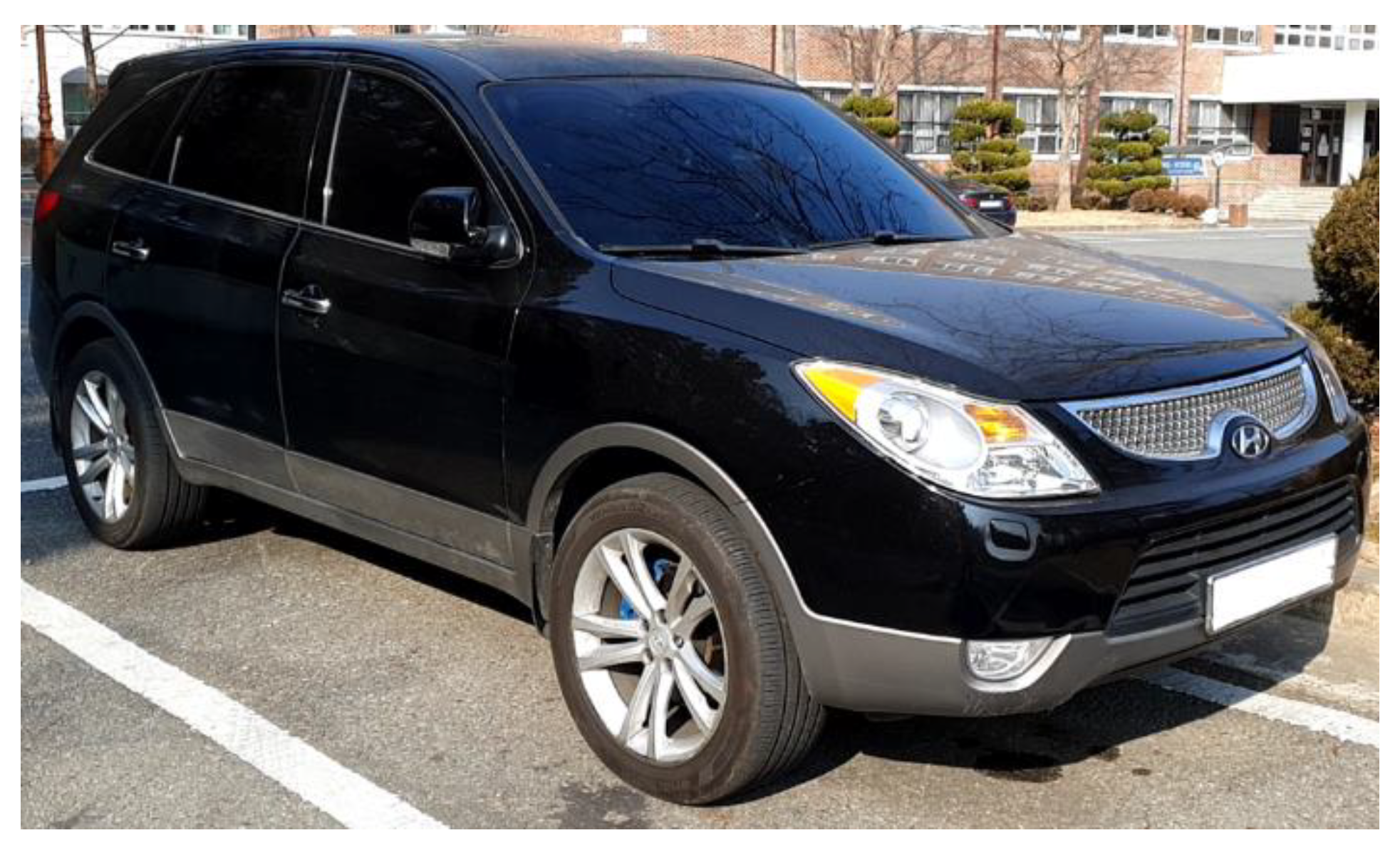
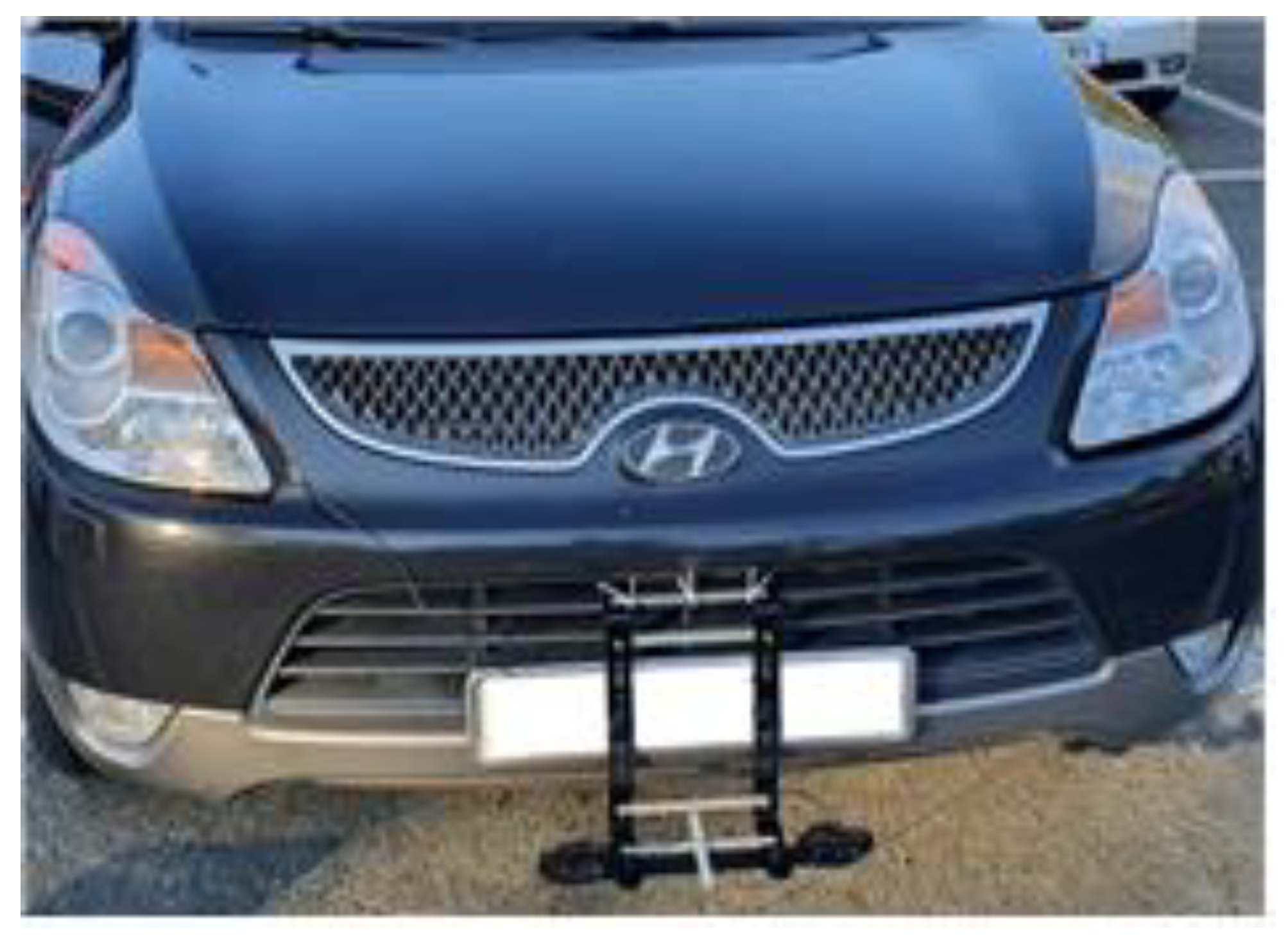
5.1. Vehicle Used for Vehicle Test

The vehicle test was conducted to verify the accuracy of the forward distance measurement equation after mounting the dual camera setup at the optimized positions. H company’s Veracruz (Figure 14) was used as the test vehicle, and its specifications are listed in

Table 2. Specifications of the test vehicle.

Name	Specification
Veracruz (vehicle)	Overall length: 4840 mm
	Overall width: 1970 mm
	Overall height: 1795 mm
	Wheel base: 2805 mm
	Tread: 1670 mm

.

The dual cameras were mounted on the front bumper of the vehicle used for the test, as depicted in Figure 15. Each camera was a Logitech C920 HD Pro Webcam, and its specifications are listed in

Table 3. Specifications of cameras.

Name	Specification
C920 HD pro webcam (camera)	height: 43.3 mm
	width: 94 mm
	depth: 71 mm
	field of view: 78°
	field of view (horizontal): 70.42°
	field of view (vertical): 43.3°
	image resolution: 1920 × 1080 p
	focal length: 3.67 mm

.

5.2. Vehicle Test Location and Conditions

Because of safety considerations, the vehicle test was conducted within the Seongseo Campus of Keimyung University, located in Daegu Metropolitan City, Korea. Figure 16 depicts the straight and curved roads utilized for testing. The radius of curvature of the curved road was 69 m; it was calculated as the radius of a planar curve based on the design speed defined in article 19 of the rules for the structure and facility standards of roads, which are presented in

Table 4. Minimum radius of curvature for curved roads according to the design standards.

Velocity (km/h)	Minimum Radius of Curve According to Maximum Slope (m)
	6%	7%	8%
120	710	670	630
110	600	560	530
100	460	440	420
90	380	360	340
80	280	265	250
70	200	190	180
60	140	135	130
50	90	85	80

. A curved road with a radius of curvature of at most 80 m was selected, considering the driving speed limit of 50 km/h in the city.

In the case of the straight road, stationary and driving states were classified using obstacles installed at intervals of 10 m between distances of 10 m and 40 m in front of the vehicle. In the case of the curved road, the two states were classified using obstacles installed at 5 m intervals between 6 m and 21 m in front of the vehicle along the center of the road and on the left and right lane markers. The entire test was conducted corresponding to a total of four cases.

The tests were repeated three times using the same equipment to acquire objective data. The environmental conditions during the experiments are summarized in

Table 5. The environmental conditions.

Item	Condition
Road	flat, dry asphalt
Weather	sunny
Temperature (°C)	9–12

. There was no variation in the weather.

5.3. Test Results

The vehicle test was conducted corresponding to four cases of stationary and driving states on the straight and curved roads. Figure 17 depicts the post-correction images captured by the dual-camera setup used to measure the distance to the object in front of the vehicle.

Table 6. Test result analysis.

Scenario	Case	Real Distance (cm)	Calculated Distance (cm)	Error Rate (%)
Straight road, Stationary state	1	1000	1008	0.78
		2000	1975	1.24
		3000	2931	2.29
		4000	4032	0.81
	2	1000	1001	0.08
		2000	1960	1.98
		3000	3083	2.77
		4000	3925	1.87
	3	1000	1004	0.41
		2000	1973	1.36
		3000	3106	3.54
		4000	3956	1.09
Straight road, Driving state	1	1060	1053	0.65
		2060	2066	0.31
		3060	-	-
		4060	-	-
	2	1060	1004	5.32
		2060	2066	0.31
		3060	-	-
		4060	-	-
	3	1060	1080	1.86
		2060	2170	5.35
		3060	-	-
		4060	-	-
Curved road, Stationary state	1	620	614	0.96
		1120	1111	0.80
		1620	1602	1.11
		2120	2085	1.65
	2	620	632	3.63
		1120	1098	1.06
		1620	1630	1.26
		2120	2303	9.13
	3	620	562	7.89
		1120	1037	6.55
		1620	1618	0.50
		2120	2084	3.67
Curved road, Driving state	1	620	562	9.40
		1120	1037	7.44
		1620	1746	7.79
		2120	-	-
	2	620	585	4.12
		1120	1063	4.28
		1620	1680	4.36
		2120	-	-
	3	620	562	9.39
		1120	1037	7.44
		1620	1746	7.79
		2120	-	-

summarizes the deviations of the theoretically calculated distances from the actual distances.

In the case of the stationary state on the straight road, the objects placed at various distances in front of the vehicle were identified. The maximum error was observed to be 3.54%, corresponding to the 30 m point.

In the case of the driving state on the straight road, the objects at distances of 10 m and 20 m in front of the vehicle were identified, whereas those farther away were not. This can be attributed to factors such as vehicular turbulence, variations in illumination, and transmission of vibration to the cameras, caused by the driving state. The maximum error was observed to be 5.35% at the 20 m point.

In the case of the stationary state on the curved road, the objects at distances between 5 m and 20 m in front of the vehicle were identified. The maximum error was observed to be 9.13%, corresponding to the 20 m point.

In the case of the driving state on the curved road, the objects at distances between 5 m and 15 m in front of the vehicle were identified, whereas those at a distance of 20 m were not. Similar to the case of the straight road, this was attributed to factors such as vehicular turbulence, variations in illumination, and transmission of vibrations to cameras. The maximum error was observed to be 9.40%, corresponding to the 6 m point.

The test results demonstrate that the error in the measurement of the distance between the vehicle and objects in front of it increases when the object is detected inaccurately owing to factors such as vehicular turbulence, variations in illumination, and transmission of vibrations to the cameras. Furthermore, the error tends to be relatively large in the case of the driving state on a curved road compared with that on a straight road; this error is affected by the fixed radius of curvature used in the calculation process.

6. Conclusions

In this study, correction of camera images and lane detection on roads were performed for vehicle tests and evaluation. Furthermore, the mounting positions of cameras were optimized in terms of three variables: height, baseline, and angle of inclination. Equations to measure the distance to an object in front of the vehicle on straight and curved roads were proposed. These were validated via the vehicle tests by classifying stationary and driving states. The results are summarized below:

(1)

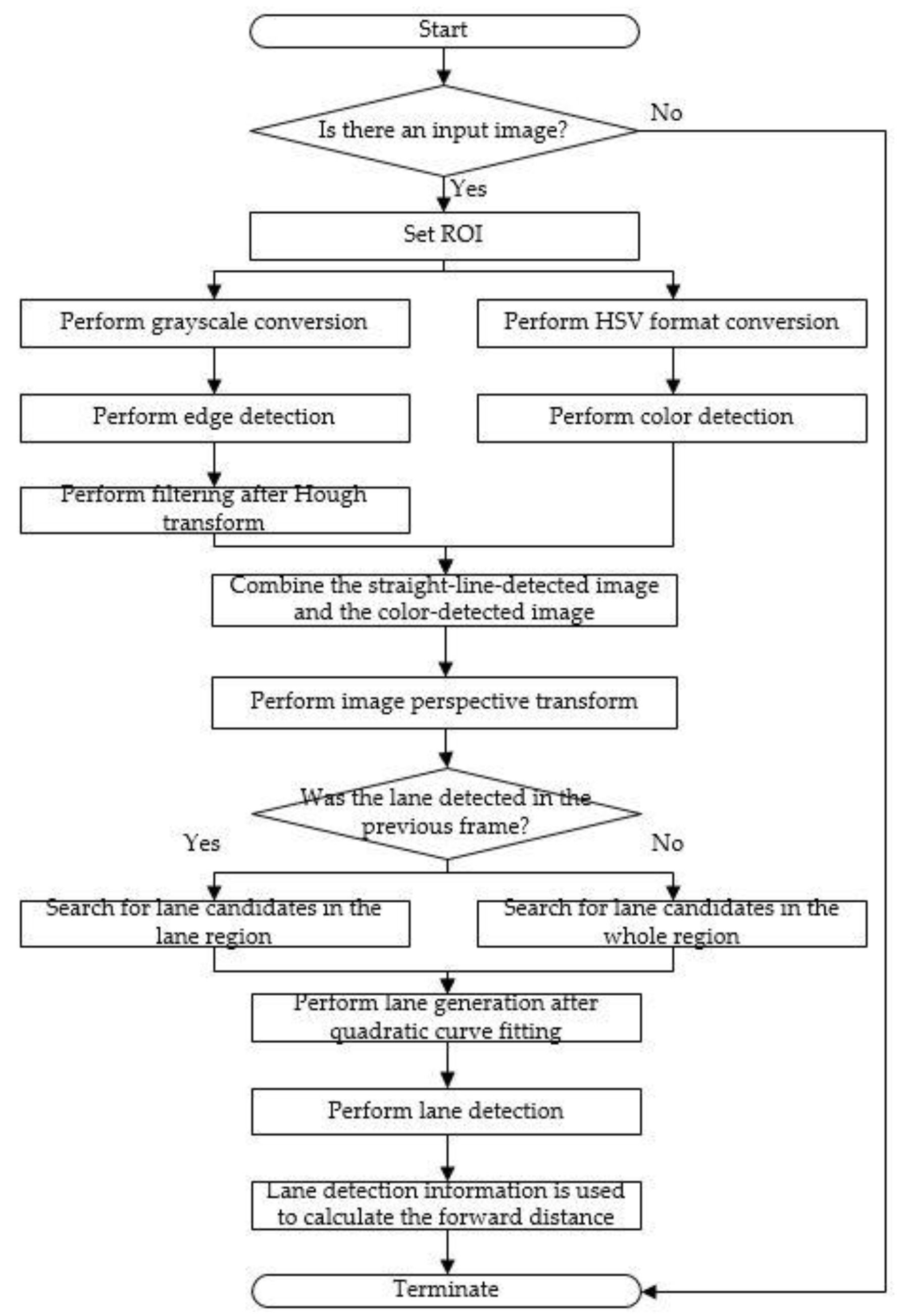
Dual camera images were used for lane detection. The ROI was selected so as to reduce the duration required for image processing, and the yellow color was extracted to HSV channels. Then, the result was combined with a grayscale conversion of the input image. Following edge detection using the Canny edge detector, the Hough transform was used to obtain the initial and final points of each straight line. After calculating the gradients of the straight lines, the lane was filtered and determined.

(2)

Height, inter-camera baseline, and angle of inclination were considered as variables for optimizing the mounting positions of the dual cameras on the vehicle. Vehicle tests were conducted on actual roads after mounting the dual cameras on a real vehicle. The test results revealed that the error rate was the smallest (0.86%), corresponding to a height of 40 cm, a baseline of 30 cm, and an angle of 12°. Hence, this was considered to be the optimal position.

(3)

Theoretical equations were proposed for the measurement of the distance between the vehicle and an object in front of it on straight and curved roads. The dual cameras were mounted on the identified optimal positions to validate the proposed equations. Vehicle tests were conducted corresponding to stationary and driving states on straight and curved roads. On the straight road, maximum error rates of 3.54% and 5.35% were observed corresponding to the stationary and driving states, respectively. Meanwhile, on the curved road, the corresponding values were 9.13% and 9.40%, respectively. Because the error rates were less than 10%, the proposed equation for the measurement of the distance to objects in front of a vehicle was considered to be reliable.

To summarize, the mounting positions of the cameras were optimized via vehicle tests using the dual cameras, and image correction and lane detection were performed. Furthermore, the proposed theoretical equation for measuring the distance between the vehicle and objects in front of it was verified via vehicle tests, with obstacles placed at the selected positions.

The aforementioned results are significant for the following reasons. These results establish that expensive equipment and professional personnel are not required for autonomous vehicle tests, enabling research and development focused on facilitating autonomous driving using only cameras as sensors. Furthermore, webcams with easy availability can also be applied without additional sensors to the testing and evaluation of autonomous driving. In the future, we expect tests to be conducted on ACC, LKAS, and HDA at the respective levels of vehicle automation.

References

1. On-Road Automated Driving (ORAD) Committee. J3016_202104: Taxonomy and Definitions for Terms Related to Driving Automation Systems for On-Road Motor Vehicles; SAE International: Warrendale, PA, USA, 2021; pp. 4–29. [Google Scholar]
2. Kee, S.C. A study on the technology trend of autonomous vehicle sensor. TTA J. 2017, 10, 16–22. [Google Scholar]
3. Lee, S.; Lee, S.; Choi, J. Correction of radial distortion using a planar checkerboard pattern and its image. IEEE Trans. Consum. Electron. 2009, 55, 27–33. [Google Scholar] [CrossRef]
4. Habib, A.; Mazaheri, M.; Lichti, D. Practical in situ implementation of a multicamera multisystem calibration. J. Sens. 2018, 2018, 1–12. [Google Scholar] [CrossRef] [Green Version]
5. Kim, H.Y.; Lee, S.B. A study on image processing algorithms for improving lane detectability at night based on camera. Trans. Korea Soc. Automot. Eng. 2013, 21, 51–60. [Google Scholar] [CrossRef]
6. Kim, J.S.; Moon, H.M.; Pan, S.B. Lane detection based open-source hardware according to change lane conditions. Smart Media J. 2017, 6, 15–20. [Google Scholar]
7. Choi, Y.G.; Seo, E.Y.; Suk, S.Y.; Park, J.H. Lane detection using gaussian function based RANSAC. J. Embed. Syst. Appl. 2018, 13, 195–204. [Google Scholar] [CrossRef]
8. Kalms, L.; Rettkowski, J.; Hamme, M.; Göhringer, D. Robust lane recognition for autonomous driving. In Proceedings of the IEEE 2017 Conference on Design and Architectures for Signal and Image Processing, Dresden, Germany, 27–29 September 2017; pp. 1–6. [Google Scholar] [CrossRef]
9. Wang, Z.; Wang, X.; Zhao, L.; Zhang, G. Vision-based lane departure detection using a stacked sparse autoencoder. Math. Probl. Eng. 2018, 2018, 1–15. [Google Scholar] [CrossRef]
10. Andrade, D.C.; Bueno, F.; Franco, F.R.; Silva, R.A.; Neme, J.H.Z.; Margraf, E.; Omoto, W.T.; Farinelli, F.A.; Tusset, A.M.; Okida, S.; et al. A novel strategy for road lane detection and tracking based on a vehicle’s forward monocular. Trans. Intell. Transp. Syst. 2019, 20, 1497–1507. [Google Scholar] [CrossRef]
11. Bae, B.G.; Lee, S.B. A study on calculation method of distance with forward vehicle using single-camera. In Proceedings of the Symposium of the Korean Institute of Communications and Information Sciences, Korea Institute of Communication Sciences, Jeju, Korea, 19–21 June 2019; pp. 256–257. [Google Scholar]
12. Park, M.; Kim, H.; Choi, H.; Park, S. A study on vehicle detection and distance classification using mono camera based on deep learning. J. Korean Inst. Intell. Syst. 2019, 29, 90–96. [Google Scholar] [CrossRef]
13. Huang, L.; Zhe, T.; Wu, J.; Wu, Q.; Pei, C.; Chen, D. Robust inter-vehicle distance estimation method based on monocular vision. IEEE Access 2019, 7, 46059–46070. [Google Scholar] [CrossRef]
14. Zhe, T.; Huang, L.; Wu, Q.; Zhang, J.; Pei, C.; Li, L. Inter-vehicle distance estimation method based on monocular vision using 3D detection. IEEE Trans. Veh. Technol. 2020, 69, 4907–4919. [Google Scholar] [CrossRef]
15. Bougharriou, S.; Hamdaoui, F.; Mtibaa, A. Vehicles distance estimation using detection of vanishing point. Eng. Comput. 2019, 36, 3070–3093. [Google Scholar] [CrossRef]
16. Kim, S.J. Lane-Level Positioning using Stereo-Based Traffic Sign Detection. Master’s Thesis, Kyungpook National University, Daegu, Korea, February 2016. [Google Scholar]
17. Seo, B.G. Performance Improvement of Distance Estimation Based on the Stereo Camera. Master’s Thesis, Seoul National University, Seoul, Korea, February 2014; pp. 1–36. [Google Scholar]
18. Kim, S.H.; Ham, W.C. 3D distance measurement of stereo images using web cams. IEMEK J. Embed. Syst. Appl. 2008, 3, 151–157. [Google Scholar]
19. Song, W.; Yang, Y.; Fu, M.; Li, Y.; Wang, M. Lane detection and classification for forward collision warning system based on stereo vision. IEEE Sens. J. 2018, 18, 5151–5163. [Google Scholar] [CrossRef]
20. Sie, Y.D.; Tsai, Y.C.; Lee, W.H.; Chou, C.M.; Chiu, C.Y. Real-time driver assistance systems via dual camera stereo vision. In Proceedings of the 2019 IEEE 89th Vehicular Technology Conference, IEEE, Kuala Lumpur, Malaysia, 28 April 2019; pp. 1–6. [Google Scholar] [CrossRef]
21. Sappa, A.D.; Dornaika, F.; Ponsa, D.; Geronimo, D.; Lopez, A. An efficient approach to onboard stereo vision system pose estimation. IEEE Trans. Intell. Transp. Syst. 2008, 9, 476–490. [Google Scholar] [CrossRef]
22. Yang, L.; Li, M.; Song, X.; Xiong, Z.; Hou, C.; Qu, B. Vehicle speed measurement based on binocular stereovision system. IEEE Access 2019, 7, 106628–106641. [Google Scholar] [CrossRef]
23. Zaarane, A.; Slimani, I.; Okaishi, W.A.; Atouf, I.; Hamdoun, A. Distance measurement system for autonomous vehicles using stereo camera. Array 2020, 5, 1–7. [Google Scholar] [CrossRef]
24. Cafiso, S.; Graziano, A.D.; Pappalardo, G. In-vehicle stereo vision system for identification of traffic conflicts between bus and pedestrian. J. Traffic Transp. Eng. 2017, 4, 3–13. [Google Scholar] [CrossRef]
25. Wang, H.M.; Ling, H.Y.; Chang, C.C. Object detection and depth estimation approach based on deep convolution neural networks. Sensors 2021, 21, 4755. [Google Scholar] [CrossRef]
26. Lin, H.Y.; Dai, J.M.; Wu, L.T.; Chen, L.Q. A Vision based driver assistance system with forward collision and overtaking detection. Sensors 2020, 20, 5139. [Google Scholar] [CrossRef]
27. Canny, J. A Computational approach to edge detection. IEEE Trans. Pattern Anal. Mach. Intell. 1986, PAMI-8, 679–698. [Google Scholar] [CrossRef]
28. Ilingworth, J.; Kittler, J. A survey of the hough transform. Comput. Vis. Graph. Image Process. 1988, 44, 87–116. [Google Scholar] [CrossRef]
29. Lee, J.Y. Camera calibration and distortion correction. Korea Robot. Soc. Rev. 2013, 10, 23–29. [Google Scholar]
30. Kim, S.I.; Lee, J.S.; Shon, Y.W. Distance measurement of the multi moving objects using parallel stereo camera in the video monitoring system. J. Korean Inst. Illum. Electr. Install. Eng. 2014, 18, 137–145. [Google Scholar] [CrossRef]
Figure 1. Flowchart of lane detection algorithm.
Energies 14 04857 g001
Figure 2. Illustration of the steps involved in lane detection: (a) the input image, (b) selection of the appropriate ROI in the input image, (c) the image obtained via grayscale conversion, (d) the edge-detected image, (e) the image obtained via filtering following Hough transform, (f) the color-detected image after conversion into the HSV format, (g) the combination of the straight-line-detected image and the color-detected image, (h) the identified lane following the perspective transform, (i) the generated lane following quadratic curve fitting, (j) the final lane-detected image.
Energies 14 04857 g002
Figure 3. Checkerboard images utilized for distortion correction: (a) identification of the corner points in the checkerboard, (b) the output image.
Energies 14 04857 g003
Figure 4. Image rectification: (a) the input image, (b) the output image.
Energies 14 04857 g004
Figure 5. Parallel stereo camera model.
Energies 14 04857 g005
Figure 6. Input images corresponding to different heights: (a) corresponding to a height of 30 cm, (b) corresponding to a height of 40 cm, and (c) corresponding to a height of 50 cm.
Energies 14 04857 g006
Figure 7. Input images corresponding to various baselines: (a) corresponding to a baseline of 10 cm, (b) corresponding to a baseline of 20 cm, (c) and corresponding to a baseline of 30 cm.
Energies 14 04857 g007
Figure 8. Input images corresponding to different angles: (a) corresponding to an angle of 3°, (b) corresponding to an angle of 7°, and (c) corresponding to an angle of 12°.
Energies 14 04857 g008
Figure 9. Test results with respect to varying baselines and angles at a height of 30 cm: (a) error rates corresponding to various angles and a baseline of 10 cm, (b) error rates corresponding to various angles and a baseline of 20 cm, (c) error rates corresponding to various angles at a baseline of 30 cm.
Energies 14 04857 g009
Figure 10. Test results with respect to varying baselines and angles at a height of 40 cm: (a) error rates corresponding to various angles and a baseline of 10 cm, (b) error rates corresponding to various angles and a baseline of 20 cm, (c) error rates corresponding to various angles and a baseline of 30 cm.
Energies 14 04857 g010
Figure 11. Test results with respect to various baselines and angles at a height of 50 cm: (a) error rates corresponding to various angles and a baseline of 10 cm, (b) error rates corresponding to various angles and a baseline of 20 cm, (c) error rates corresponding to various angles and a baseline of 30 cm.
Energies 14 04857 g011
Figure 12. Distance to the object in front of the vehicle on a straight road.
Energies 14 04857 g012
Figure 13. Distance to the object in front of the vehicle on a curved road.
Energies 14 04857 g013
Figure 14. Test vehicle.
Energies 14 04857 g014
Figure 15. Test device.
Energies 14 04857 g015
Figure 16. Vehicle test roads: (a) straight road, (b) curved road.
Energies 14 04857 g016
Figure 17. Test result images: (a) on the straight road, (b) on the curved road.
Energies 14 04857 g017