Practically-Achievable Energy Savings with the Optimal Control of Stratified Water Heaters with Predicted Usage

Abstract

Residential water heaters use a substantial amount of electrical energy and contribute to 25% of the energy usage in the residential sector. This raises concern for users in countries with flat rate electricity fees and where fossil fuels are used for electricity generation. Demand side management of tanked water heaters is well suited for energy-focused load reduction strategies. We propose a strategy for providing an electric water heater (EWH) with the optimal temperature planning to reduce the overall electrical energy usage while satisfying the comfort of the user. A probabilistic hot water usage model is used to predict the hot water usage behaviour for the A*-based optimisation algorithm, which accounts for water stratification in the tank. A temperature feedback controller with novel temperature and energy-correcting capabilities provides robustness to prediction errors. Three optimal control strategies are presented and compared to a baseline strategy with the thermostat always on: The first ensures temperature-matched water usages, the second ensures energy-matched water usages, and the third is a variation of the second that provides Legionella prevention. Results were obtained for 77 water heaters, each one simulated for four weeks. The median energy savings for predicted usage were $2.2$% for the temperature-matched strategy, and $9.6$% for both of the energy-matched strategies. We also compare the practical energy savings to the ideal scenario where the optimal scheduling has perfect foreknowledge of hot water usages, and the temperature and energy-matched strategies had a 4.1 and 11.0 percentage point decrease from the ideal energy savings.

1. Introduction

Energy usage by domestic water heaters can be reduced by optimal control strategies. These take into account the pattern of actual hot water usage and the user’s convenience. However, the savings have only been demonstrated and quantified using optimisation for unstratified thermal models, and with perfect foreknowledge of the hot water usage patterns. Stratification, i.e., layers of different temperatures in the tank because of the different densities of cold and hot water, is known to occur in water heaters. A control strategy that takes this into account could well improve the savings.

Much of the household electricity demand is as a result of water heating [1,2]. Water heating accounts for 18% of the residential energy consumption in the USA and 25% in the UK [3,4]. Furthermore, the residential energy used in the USA accounts for 20% of their greenhouse gas emissions [5].

Water heaters supply water, and consequently energy, in a cyclical pattern. This provides the possibility of shifting peak loads for demand side management (DSM) strategies. Those with storage tanks are particularly suitable because they can conserve thermal energy for long times with relatively little heat loss [6].

The thermal energy they retain can be stored for delayed use in schemes that schedules the supply of power for peak-shifting [7,8,9]. Such schemes must take into account the heater’s thermal behaviour, and the customer’s water draw behaviour and satisfaction [10,11]. Literature studies relating to smart grid applications have thoroughly covered the thermal models and control algorithms for water heaters [7,9,10,12,13,14,15,16,17,18,19,20,21,22,23,24,25,26,27]. However, very few studies have proposed models explicitly designed for water heating to achieve an overall reduction of energy usage. Most have proposed models designed to manage peak load by optimising the time-of-use pricing to provide benefits for the generator of the customer.

Users in some countries, typically paying a time-dependent flat fee for power rather than tariffs that are based on congestion or time-of-use, decrease their costs per month by turning to schedule control [1,28]. These users contribute to increasing energy usage as a result of DSM strategies [11]. Demand response strategies that focus on reducing the total energy consumption of a household can therefore reduce costs and minimise greenhouse gas emissions.

In this paper, we focus on achieving general energy savings by optimal temperature and schedule control instead of cost savings where congestion charges are avoided.

A fundamental driver of energy usage and available savings of a water heater is the hot water draw profile [29].

In a recent study, Braas et al. [30] developed a method for generating heat profiles for domestic water heaters to find the most cost-efficient heating solution. They note the importance of draw-off profiles and appropriate time intervals. Ref. [31], reviewing the current state of work on improving the energy performance of domestic water heaters, highlights the importance of measured energy data and spatial distribution of water usage for optimisation, and they note that advanced control strategies can cleverly adjust heating systems to decrease energy loss, increase user comfort and minimise Legionella risks. Legionella bacteria can flourish in water heaters at lower water temperatures. They pose a health risk to humans, causing diseases collectively referred to as Legionellosis [32].

Roux et al. [11] found that schedule control had the largest effect when simulating a variety of hot water draw patterns, where a one-node water heater model was used, and achieving energy savings of 9–18%.

Whereas existing papers assess savings for perfect foreknowledge of the hot water usage patterns, this paper uses predicted knowledge to assess the performance under practical conditions of uncertain usage. The objective is to determine the practical electrical energy savings by predicting the hot water usage profile. However, hot water usage patterns are difficult to predict accurately as water draw behaviour is unique to each household and varies over time. To tackle these issues, a probabilistic hot water usage model produces predicted hot water usages that accounts for these factors and is solved with the optimisation algorithm.

1.1. Challenges in Literature

This section summarises the challenges remaining in literature, highlighting the research gaps remaining in this paper. We review the studies and describe their data, methods and results (energy savings), and any limitations or shortcomings.

Fanney and Dougherty [33] evaluate electrical water heater thermal efficiency. They perform six simulations of water usage profiles with varying heating schedules. However, they use thermal efficiency as a standalone metric for assessing energy savings. This is not ideal because the efficiency of the water heater varies for high and low volumes of usage, and, if it is switched off, it has a thermal efficiency of 100%. They predict savings of 4% and 6%, but their actual energy savings were not explicitly stated.

Goh and Apt [12], Gholizadeh and Aravinthan [10], Booysen et al. [16], Nel et al. [19], Booysen and Cloete [34] and Cloete [35] use schedule control to evaluate the electrical energy savings.

Using hourly water usage profiles, Goh and Apt [12] find 5–8% savings. Gholizadeh and Aravinthan [10] yield 5.9–6.4% energy savings with additional control of the temperature. They generate water usages based on the ASHRAE 90.2 water profile standard. However, the water profile is too general and does not account for the variety in water demand from user to user. Both studies simulate water heaters without accounting for the total energy used and outlet temperature.

Booysen et al. [16] find an energy saving of 14% to 17%. Their results are confirmed by performing an experiment. Their results are obtained using a lumped-mass analytical physics model and only one water usage profile is used. The consequences of reducing the outlet temperature of the hot water drawn are not accounted for (i.e., the reduction in energy used).

A model of water heaters with heating control based on a thermostat or scheduling is developed by Nel et al. [19] and has improved accuracy. The same model is used by Booysen and Cloete [34]. They carry out a controlled laboratory experiment using a single water heater and a controlled filed trial using four heaters and find 29% savings. They don’t determine the energy savings when the temperature and energy are matched to that of the baseline method. Cloete [35] repeats the laboratory experiment with extended heating periods. Additionally, the set-point is adjusted to match the outlet temperature to ensure a fair comparison. This caused the savings of 16% to be reduced to 6%.

Refs. [36,37] use dynamic programming for optimal schedule control.

Ref. [36] uses hourly control to minimise cost and energy usage. They use synthesised usage patterns from [38]. They find energy savings of 4.5–13.3%. Kepplinger et al. [18], their subsequent study, uses an auto-scheduling method. Similarly to the model presented in this paper, they perform simulations on a thermal model that accounts for stratification. They find energy savings of 10.5–12.4%. Although the model ensures that the energy delivered is matched, it does not ensure that the temperature at the beginning of each water usage is matched to that achieved by a water heater controlled only by a thermostat for the same usage. Kepplinger et al. [39] conduct field trials in a follow-up study. They determine savings of 12.3%. These studies use a k-nearest neighbourhood algorithm to estimate future water usage with hourly time steps.

Ref. [37] uses minutely control to minimise energy usage. They use real hot-water usage patterns. They include strategies that achieve target delivery temperatures and energy usages. They also include Legionella sterilisation. As the study is based on a one-node electric water heater model, water stratification is ignored and not reflected in the results. This study assumes perfect knowledge of future water usages.

Ref. [40] use a novel direct load control method for water heaters without the need for temperature information. They do this by using a time-varied weight matrix, generated from hourly hot water usage patterns. The matrix produces a user comfort index which determines how the water heater can be controlled to shift peak loads.

It is clear from the preceding analysis that many challenges remain. None of the existing work in literature accounted for stratification in the heater, which is expected to have a substantial impact. None of the existing literature implemented a strategy to reduce the growth of Legionella. Unless stated, the control strategies in the related work do not plan for predicted water usages that are then assessed with actual water usages. More importantly, they did not use water usage data sampled at high frequency, i.e., using minutes rather than hours. High frequency water usage profiles are required to increase the accuracy of water usage predictions and to increase the effectiveness of feedback control mechanisms to correct potential prediction errors. Because of the randomness of water draw behaviour, incorrect water usage predictions are a common occurrence. However, none of the studies account for correcting the EWH temperature when prediction errors occur. These studies also do not use a validated water usage model that accounts for factors that influence a household’s water usage behaviour, such as the users unique behaviour and temporal variations.

1.2. Contributions

The work presented in this paper uses components from our previous papers, [41,42], and makes the following contributions:

• The residential electric water heater control problem was mathematically formulated in a novel way as an optimal control problem with the objective to find the heating element switching signal and the optimal temperature state trajectory to minimise the energy used, while satisfying an anticipated hot water usage profile.
• A novel A*-based technique was developed that solves the optimal control problem using a two-node lumped parameter model of the electric water heater that takes stratification into account.
• A novel feedback control technique was developed that controls the temperature inside the electric water heater to follow the planned optimal temperature trajectory, rejecting disturbances such as unanticipated hot water usage and providing robustness to model uncertainty.
• A novel hot water usage model was developed that uses clustering and statistical analysis to model the user’s temporal hot water usage behaviour based on historically measured usage data. The hot water usage model is used to predict the anticipated hot water usage profile for the optimal control algorithm.
• A reactive hot water usage simulation model was developed that generates a synthetic hot water usage profile with random variations based on the clustering and statistical properties of the historical usage data. The model simulates the fact that the user will adjust the ratio of cold water and hot water mixing based on the temperature of the hot water.
• A study was performed to determine how much energy can practically be saved with optimal control for electric water heaters compared to the traditional thermostat control.

In our previous paper, Engelbrecht et al. [42], we investigated how much energy can theoretically be saved with optimal control for electric water heaters compared to traditional thermostat control, when perfect foreknowledge of the hot water usage profile is available. The probabilistic hot water usage model and the hot water usage predictor were therefore not used in the paper, but perfect foreknowledge of the hot water usage profile was used instead. In this paper, we investigate the practical energy savings that are achievable with usage-based optimal energy control, when a predicted hot water usage profile based on historically measured data are used. This paper therefore includes the probabilistic hot water usage model and the hot water usage predictor.

2. System

2.1. System Overview

The goal of the system described in this paper is to minimise the electrical energy used by a storage-based electric water heater (EWH) while preventing the user from experiencing cold water temperatures, for a given predicted hot water usage profile. An overview of the system is shown in Figure 1. The system consists of an optimal temperature schedule planner, a temperature feedback controller, a probabilistic hot water usage model and a hot water usage predictor. The EWH is modelled using a two-node thermodynamic model that accounts for stratification. The EWH is controlled by a heating element that can be switched either on or off. The user is modelled using a reactive hot water usage model that simulates the user experiencing the outlet temperature of the hot water and adjusting the mixing ratio of hot and cold water to obtain the desired temperature.

The optimal control sequence for the heating element and the corresponding optimal EWH temperature trajectory are determined by an optimal temperature schedule planner. A two-node EWH model that accounts for water stratification is used, and the optimal control problem is solved using an A* search algorithm, as described in this paper.

The temperature feedback controller is used to compensate for deviations between the planned optimal temperature trajectory and the actual temperature trajectory, rejecting disturbances such as unanticipated hot water usage and providing robustness to model uncertainty. The temperature feedback controller controls the water temperature inside the EWH to follow the temperature set point provided by the optimal temperature planner by switching the heating element based on feedback from the EWH internal temperature sensor.

The optimal schedule planner uses a predicted hot water usage profile to plan the optimal EWH temperature trajectory. The predicted hot water usage profile is provided by the hot water usage predictor, which in turn uses a probabilistic hot water usage model. The probabilistic hot water usage model is obtained by fitting a probabilistic model to historical measured hot water usage data obtained from the EWH temperature and flow rate sensors [41]. The probabilistic hot water usage model and the hot water usage predictor will generate predicted hot water usage profiles for which the optimal heating schedule will be planned.

2.2. Heating Control Strategies

We use the following four heating control strategies in this paper. The first strategy is traditional thermostat control that serves as the baseline against which we will evaluate the energy savings achieved by the three variations of our optimal control strategy.

0. Thermostat control (TC): This strategy is typically used by most people and is the operation for the intended design. The thermostat with a set-point temperature, usually around 70 ${}^{\circ }\mathrm{C}$ (with small hysteresis), maintains the target water temperature. The strategy is inefficient and wasteful since the water is maintained at the set-point temperature when hot water is not drawn for long time periods. This results in substantially more energy lost to the environment compared to the other strategies. Furthermore, the user normally requires a temperature of about 40 ${}^{\circ }\mathrm{C}$ and will therefore adjust the mixing of hot and cold water to obtain the desired water temperature [26,43,44].

1. Temperature-matched scheduled control (TM): The energy losses and costs have been reduced by some users by switching off the water heater during long periods when they are not needed, and ideally switching it on shortly before hot water is needed again [16,28]. The operation of this strategy provides optimal control of the heating element switching sequence to minimise thermal losses and ensuring that water is drawn at the same volume and temperature (and delivering an equivalent amount of output energy) as that of thermostat control. Similarly to thermostat control, the strategy assumes that the user will adjust the water mixer to reach their desired temperature.

2. Energy-matched scheduled control (EM): This strategy reduces the need for the user to add cold water to obtain their desired water temperature (assuming 40 ${}^{\circ }\mathrm{C}$) by lowering the target temperature during water usages. However, a delivery of the same amount of energy to that of thermostat control is ensured by increasing the volume of water drawn from the tank [11,43,44].

3. Energy-matched scheduled control with Legionella prevention (EML): While the previous strategy saves energy, maintaining low water temperatures for long periods of time can introduce health risks. Legionella pneumophila can be found in water heaters and thrives at water temperatures between 32 ${}^{\circ }\mathrm{C}$ and 42 ${}^{\circ }\mathrm{C}$ [32,43]. The bacteria can be sterilised if the water heater maintains a temperature of 60 ${}^{\circ }\mathrm{C}$ for 11 min [45]. This strategy is a modification of the previous one that implements an additional optimisation constraint that ensures the sterilisation of this bacteria.

2.3. Electric Water Heater Thermodynamics

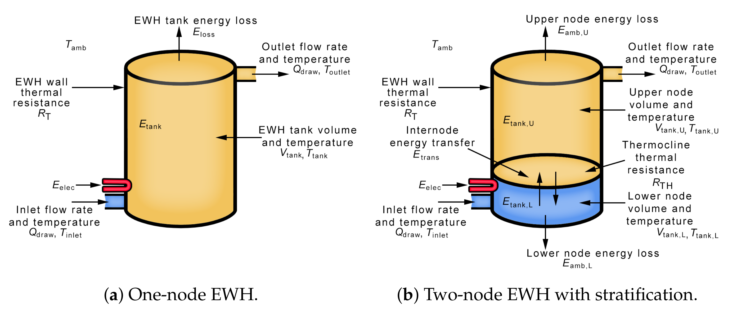
The EWH thermodynamics can be modelled using a one-node or two-node lumped-mass model. The latter models stratification. In this paper, we consider only a vertically oriented tank. A horizontally oriented tank can also be considered but requires substantially more computational power to implement the model that is used for the optimal temperature planning Nel [46]. The EWH is modelled according to an energy balance equation to track the energy flow in the tank. In the one-node model, the body of water inside the tank is assumed to be at a uniform temperature, as shown in Figure 2a. Energy flows into the tank from an electrical heating element situated near the base of the tank. If warm water leaves the tank at a higher temperature than the water in the inlet pipe, the thermal energy of the tank decreases due to the volumetric flow rate. When the temperature of the tank water is different to the ambient temperature, thermal energy is lost from the tank at a rate determined by the tank’s thermal resistance.

The two-node EWH in Figure 2b models stratification by introducing a thermocline that divides the tank into an upper and a lower node which represent the hot and cold water, respectively. Water leaving the outlet pipe is at the temperature of the upper node and water entering the inlet pipe is at the ambient temperature. Inter-node energy transfer occurs due to the temperature difference at the thermocline between the two bodies of water at a rate determined by the thermal resistance of the thermocline. The full description of the EWH dynamics used in this paper can be found in Ritchie [47].

2.3.1. One-Node EWH Dynamics

We express the thermal dynamics of the one-node EWH model as follows:

$${\dot{E}}_{\mathrm{tank}}\left(t\right)=P_{\mathrm{elec}}\left(t\right)-P_{\mathrm{draw}}\left(t\right)-P_{\mathrm{loss}}\left(t\right)$$

(1)

where $E_{\mathrm{tank}}$ is the thermal energy in the tank, $P_{\mathrm{elec}}$ is the electrical power supplied by the heating element, $P_{\mathrm{draw}}$ is the power of hot water leaving the tank during usage, and $P_{\mathrm{loss}}$ is the power leaving the tank due to losses to the environment. The equation shows that the rate of change of thermal energy is directly influenced by $P_{\mathrm{elec}}$, $P_{\mathrm{draw}}$ and $P_{\mathrm{loss}}$.

2.3.2. Two-Node EWH Dynamics

When the tank is in a one-node state and water is drawn at a temperature higher than that at the inlet pipe, the tank transitions to a two-node state. When all the hot water is drawn from the tank, the EWH reverts to a one-node state and the temperature of the whole tank is that of the lower node. The EWH also transitions to a one-node state when the lower node temperature reaches the temperature of the upper node. The nodes are referred to as the upper and the lower node and are designated by subscripts U and L, respectively.

The energy and volumes of the upper and lower nodes are related to the total energy and total volume of the tank by the following equations:

$$\begin{array}{ccc}\hfill E_{\mathrm{tank}}\left(t\right)& =& E_{\mathrm{tank},\mathrm{U}}\left(t\right)+E_{\mathrm{tank},\mathrm{L}}\left(t\right)\hfill \\ \hfill V_{\mathrm{tank},\mathrm{U}}\left(t\right)+V_{\mathrm{tank},\mathrm{L}}\left(t\right)& =& V_{\mathrm{tank}}\hfill \end{array}$$

(2)

The total energy $E_{\mathrm{tank}}$ in the tank is the sum of the energy $E_{\mathrm{tank},\mathrm{U}}$ in the upper node and the energy $E_{\mathrm{tank},\mathrm{L}}$ in the lower node. The sum of the upper node volume $V_{\mathrm{tank},\mathrm{U}}$ and the lower node volume $V_{\mathrm{tank},\mathrm{L}}$ are constrained to equal the total volume of the tank $V_{\mathrm{tank}}$, which remains constant.

The thermal dynamics of the two-node EWH model is described by a set of four differential equations in terms of the upper node energy, the lower node energy, the upper node volume, and the lower node volume, respectively.

The first differential equation describes the dynamics of the upper node’s thermal energy, as follows:

$${\dot{E}}_{\mathrm{tank},\mathrm{U}}\left(t\right)=-P_{\mathrm{draw},\mathrm{U}}\left(t\right)-P_{\mathrm{loss},\mathrm{U}}\left(t\right)-P_{\mathrm{trans},\mathrm{U}}\left(t\right)$$

(4)

The rate of change of the upper node’s thermal energy ${\dot{E}}_{\mathrm{tank},\mathrm{U}}$ is the sum of the power $P_{\mathrm{draw,U}}$ leaving the upper node when hot water is drawn, the power $P_{\mathrm{loss,U}}$ leaving the upper node due to losses to the environment, and the power $P_{\mathrm{trans,U}}$ leaving the upper node due to power transfer to the lower node across the thermocline.

The second differential equation describes the dynamics of the lower node’s thermal energy:

$${\dot{E}}_{\mathrm{tank},\mathrm{L}}\left(t\right)=P_{\mathrm{elec}}\left(t\right)+P_{\mathrm{inlet},\mathrm{L}}\left(t\right)-P_{\mathrm{loss},\mathrm{L}}\left(t\right)-P_{\mathrm{trans},\mathrm{L}}\left(t\right)$$

(5)

The rate of change of the lower node’s thermal energy ${\dot{E}}_{\mathrm{tank},\mathrm{L}}$ is the sum of the electrical power $P_{\mathrm{elec}}$ delivered to the lower node by the heating element, the power $P_{\mathrm{inlet},\mathrm{L}}$ entering the lower node due to the thermal energy in the cold water flowing into the inlet, the power $P_{\mathrm{loss,L}}$ leaving the lower node due to losses to the environment, and the power $P_{\mathrm{trans,L}}$ leaving the lower node due to power transfer to the upper node across the thermocline.

The third and fourth differential equations describe the dynamics of the upper node volume and the lower node volume, as follows:

$$\begin{array}{ccc}\hfill {\dot{V}}_{\mathrm{tank},\mathrm{U}}\left(t\right)& =& -Q_{\mathrm{draw}}\left(t\right)\hfill \end{array}$$

(6)

$$\begin{array}{ccc}\hfill {\dot{V}}_{\mathrm{tank},\mathrm{L}}\left(t\right)& =& Q_{\mathrm{draw}}\left(t\right)\hfill \end{array}$$

(7)

The rate at which the upper node volume $V_{\mathrm{tank},\mathrm{U}}$ decreases and the rate at which the lower node volume $V_{\mathrm{tank},\mathrm{L}}$ increases both equal the flow rate $Q_{\mathrm{draw}}$ of the hot water leaving the tank, which also equals the flow rate of the cold water into the tank.

2.4. Temperature Feedback Control

The optimal temperature plan is passed to the temperature feedback controller before determining the input of the EWH at any given time. The controller compares the measured temperature of the EWH with the desired time-varying temperature set-point of the optimal plan. The controller will override the optimal input for the EWH so that the temperature of the EWH follows the optimal temperature (with hysteresis). The temperature feedback control corrects the EWH temperature when it deviates from the optimal plan. Temperature deviations are caused by unexpected water usages and model inaccuracies.

2.5. User and Water Mixer

The user experiences the hot water temperature of the EWH when a usage event is intended. If the initial temperature experienced by user is not the desired temperature, the user will adjust the ratio of hot and cold water using a water mixer to reach such a desired temperature. The water mixer is a model of reality and is used to perform and evaluate simulation tests. The model is also used by the energy matching heating control strategies to adjust the predicted hot water flow rate that is used to calculate the optimal temperature plan. If the predicted temperature inside the EWH differs from the user’s desired temperature during a predicted usage event, then the hot water flow rate is adjusted to reflect the user’s anticipated water mixing action.

3. Optimal Temperature Planning for an EWH with Stratification

This section presents the algorithm that performs the optimal planning for a two-node EWH model with stratification. A full description of the optimal control problem and A* algorithm that is used to solve can be found in Ritchie [47].

3.1. Formulation of the Optimal Control Problem

Given a hot water profile that represents flow rate $Q_{\mathrm{usage}}\left(t\right)$ as a function of time t and time-varying disturbance signals for the ambient and cold inlet temperature $T_{\mathrm{amb}}\left(t\right)$ and $T_{\mathrm{in}}\left(t\right)$, the EWH control problem is to find the optimal control signal $P_{\mathrm{elec}}^{*}\left(t\right)$ that minimises the overall energy usage and also satisfying the hot water usage profile. We use the following cost function to represent the objective of minimising the total energy usage:

$$\begin{array}{c}\hfill J={\int }_{t_i}^{t_f}{P}_{\mathrm{elec}}\left(t\right)dt\end{array}$$

(8)

We define constraints for the water temperature profile to satisfy the hot water profile. We set the upper node profile temperature $T_{\mathrm{tank},\mathrm{U}}\left(t\right)$ to the required water usage temperature $T_{\mathrm{usage}}$ during any time that water is drawn, the lower node profile water temperature $T_{\mathrm{tank},\mathrm{L}}\left(t\right)$ to the Legionella sterilisation temperature $T_{\mathrm{Legionella}}$ once a day, and both profiles to the minimum water temperature of the EWH $T_{\min }$ during any other time:

$$\begin{array}{c}{T}_{\mathrm{tank},\mathrm{U}}\left(t\right)\ge \left\{\begin{array}{cc}{T}_{\mathrm{usage}}\hfill & \mathrm{when\; intentional\; draw\; causes} Q_{\mathrm{draw}}\left(t\right)>0\\ T_{\min }\hfill & \mathrm{otherwise}\hfill \end{array}\right\}\hfill \end{array}$$

(9)

$$\begin{array}{c}{T}_{\mathrm{tank},\mathrm{L}}\left(t\right)\ge \left\{\begin{array}{cc}{T}_{\mathrm{Legionella}}\hfill & \mathrm{once\; per\; day\; to\; prevent} \mathit{Legionella} \mathrm{growth}\\ T_{\min }\hfill & \mathrm{otherwise}\hfill \end{array}\right\}\hfill \end{array}$$

(10)

“Unreasonable” hot water usage profiles: We account for hot water usage profiles with “unreasonable” water usages where hot water cannot be delivered at the required water usage temperature, even when the heating element is always on. As an example, this can happen when all of the hot water is drawn from the tank during a water usage and then the availability of hot water is immediately expected. Before applying the optimisation algorithm, these profiles are accounted for by performing a forward simulation of the water profile with the heating element permanently switched on. If any temperatures in the simulation fall below the desired usage temperature during water usages, the temperature profile constraints are then modified to these achievable temperatures.

The temperature profile constraints are constructed differently for each of the optimal control strategies:

Temperature-matched constraints: The constraints of the temperature profile are constructed to ensure that the outlet water temperature during the beginning of each usage matches that of thermostat control applied to the same hot water usage profile.

Energy-matched constraints: The constraints of the temperature profile are constructed to ensure that the outlet water temperature remains above 40 ${}^{\circ }\mathrm{C}$ during each water usage. By doing this, the outlet flow rate is increased to match the energy delivered by that of thermostat control (at a higher water temperature) applied to the same hot water usage profile. However, when water usages are predicted, there is always an uncertainty that the actual water usage will start earlier than what was predicted, or use a larger volume of water. This would certainly result in a cold event. A 10 ${}^{\circ }$C buffer is added to the usage constraint $T_{\mathrm{usage}}$ to provide a safety margin and greatly reduce the risk of cold events.

Energy-matched with Legionella prevention constraints: The constraints of the temperature profile are constructed for both energy matching and for preventing Legionella. The temperature of the entire tank is increased to 60 ${}^{\circ }\mathrm{C}$ for 11 min once a day. The EWH is scheduled to be heated to this temperature as soon as the biggest water usage for that day is about to occur to reduce the necessity of additional water heating.

3.2. The A* Solution

The A* algorithm is a well-known and widely-used shortest path search algorithm that can be used to model a given optimal control problem as a node-based data structure navigation process to find the optimal state trajectory and control inputs to minimise the cost function from an initial state to a destination. The algorithm optimises its search time by introducing a heuristic function that estimates the path to a terminal state. However, the efficiency of the algorithm depends on the quality of the chosen heuristic function. The A* algorithm builds a binary search tree that has two possible actions at each node: element on and element off.

Discretisation

If we desire to apply A* to a given optimal control problem, we have to break the problem into discrete time instants that represent the different decision stages, and into discrete states that represent the allowable decisions to be determined at any decision stage. The A* algorithm finds the optimal path by starting at the initial stage and working through intermediate stages until it finds the first admissible path from the initial state to a terminal state. The first admissible path is also the optimal path due to the way that the paths are sorted in a priority queue.

The continuous-time differential equations describing the system dynamics are discretised to produce discrete-time difference equations that describe the state transition from one discrete time instant to the next.

For the one-node case, the state transition is described as

$$\begin{array}{ccc}\hfill E(k+1)& =& E\left(k\right)+[P_{\mathrm{elec}}\left(k\right)-P_{\mathrm{usage}}\left(k\right)-P_{\mathrm{losses}}\left(k\right)]\Delta t\hfill \end{array}$$

(11)

where $\Delta t$ is the sampling period of the discrete time instant.

For the two-node case, the state transition is described by the following set of difference equations:

$$\begin{array}{ccc}\hfill E_{\mathrm{U}}(k+1)& =& E_{\mathrm{U}}\left(k\right)+{\dot{E}}_{\mathrm{U}}\left(k\right)\Delta t\hfill \end{array}$$

(12)

$$\begin{array}{ccc}\hfill E_{\mathrm{L}}(k+1)& =& E_{\mathrm{L}}\left(k\right)+{\dot{E}}_{\mathrm{L}}\left(k\right)\Delta t\hfill \end{array}$$

(13)

$$\begin{array}{ccc}\hfill V_{\mathrm{tank},\mathrm{U}}(k+1)& =& V_{\mathrm{tank},\mathrm{U}}\left(k\right)-Q_{\mathrm{draw}}\left(k\right)\Delta t\hfill \end{array}$$

(14)

where ${\dot{E}}_{\mathrm{U}}\left(k\right)$ and ${\dot{E}}_{\mathrm{L}}\left(k\right)$ are respectively given as

$$\begin{array}{ccc}\hfill {\dot{E}}_{\mathrm{U}}\left(k\right)& =& -P_{\mathrm{draw},\mathrm{U}}\left(k\right)-P_{\mathrm{loss},\mathrm{U}}\left(k\right)-P_{\mathrm{trans},\mathrm{U}}\left(k\right)\hfill \end{array}$$

(15)

$$\begin{array}{ccc}\hfill {\dot{E}}_{\mathrm{L}}\left(k\right)& =& P_{\mathrm{elec}}\left(k\right)+P_{\mathrm{inlet},\mathrm{L}}\left(k\right)-P_{\mathrm{loss},\mathrm{L}}\left(k\right)-P_{\mathrm{trans},\mathrm{L}}\left(k\right)\hfill \end{array}$$

(16)

The lower node volume is calculated by subtracting the upper node volume from the constant total volume of the tank, as follows:

$$V_{\mathrm{tank},\mathrm{L}}(k+1)=V_{\mathrm{tank}}-V_{\mathrm{tank},\mathrm{U}}(k+1)$$

(17)

The A* algorithm starts at an initial node, and will navigate through a binary search tree by producing paths of interconnected nodes until the desired goal node is reached. At each iteration, the action space for the considered node at a path ending is used to generate child nodes from the given parent node. There are two possible actions that produce two possible child nodes: when the heating element is on and off for that time sample. The algorithm repeatedly switches between calculating different search paths, and a priority queue is initialised to give priority to the path ending that is considered for the next iteration. The queue determines the priority for the paths based on a cost that is assigned to every existing node.

Total path cost: The total cost J is calculated by the cost-to-come and cost-to-go, and is calculated as follows:

$$J(k+1)=g(k+1)+h(k+1)$$

(18)

Cost-to-come: The cost-to-come is calculated incrementally as nodes are created and added to the search tree. The cost to come is the total energy use so far and is calculated with

$$\begin{array}{c}\hfill g(k+1)=g\left(k\right)+P_{\mathrm{elec}}\left(k\right)\Delta t\end{array}$$

(19)

where $g(k+1)$ is the total cost-to-come of the child node, $g\left(k\right)$ is the total cost to come of the parent node, and $P_{\mathrm{elec}}\left(k\right)\Delta t$ is the incremental energy used.

Heuristic search: A heuristic cost function is introduced to accelerate the search algorithm by prioritising the optimal path as the next iteration of the algorithm execution. This is accomplished by heuristics: estimating the path cost from the next state ${\mathbf{x}}_j(k+1)$ to the terminal state.

Cost-to-go: At any time instant, the EWH must reach the terminal state after the result of thermal energy that is anticipated to still leave the tank. The cost-to-go estimates both the minimum amount of energy that must still be supplied to the tank to reach the terminal energy state as well as how much thermal energy will leave the tank during the remaining water usages from the considered time instant. The cost-to-go is calculated with

$$h(k+1)=E(k+1)+E\left(N\right)+\sum _{n=k+1}^N{P}_{\mathrm{usage}}\left(n\right)\Delta t$$

(20)

where $E(k+1)$ is the energy at the child node, $E\left(N\right)$ is the energy at the final node, and $P_{\mathrm{usage}}\left(n\right)\Delta t$ is the predicted thermal energy that will leave the tank due to hot water usage. Because standing losses contribute a relatively small portion of the thermal energy that leaves the tank, the thermal energy loss to the environment is not included in the cost-to-go. The heuristic is still valid, however, since, by ignoring the standing losses, the heuristic underestimates the actual cost-to-go.

$P_{\mathrm{usage}}\left(n\right)\Delta t$ is the estimated thermal energy that is drawn from the tank at a specific time instant. It is pre-calculated by performing a forward simulation of the water profile which acts as a disturbance to the EWH. The simulation is performed such that each water event ends with the outlet temperature remaining above $T_{\mathrm{usage}}$.

4. Probabilistic Hot Water Usage Model and Predictor

A novel probabilistic hot water usage model was developed in Ritchie et al. [41] and a summary is presented in this section. The model uses historical data measurements to statistically model the hot water usage behaviour from day to day for an individual EWH. A hot water usage predictor is developed that implements the model to produce hot water profiles with predicted water usages for the optimisation algorithm. The A* optimisation process must prevent the user from experiencing cold water temperatures when they start using hot water. Therefore, it requires a hot water profile that predicts water usages that have the earliest expected start time and largest expected total volume to ensure a that the tank is sufficiently heated to accommodate the worst case of a water usage. The predictor is designed to generate such a water profile and is referred to as a conservative water profile.

4.1. Probabilistic Hot Water Usage Model

The development of the probabilistic hot water usage model is described in this section and the steps are shown in Figure 3. The model statistically models an individual EWH’s water draw behaviour by first grouping flow rate measurements into clusters of time, flow rate and volume, and then fitting statistical distributions to the starting time, average flow rate and total volume used for each water usage.

The model assumes that the usage behaviours differ between seasons and day of the week and separates the data into different data sets accordingly. Repeating usage events are identified by superimposing the measured flow rate data on a single day cycle, as shown in Figure 3a. Clustering is used to determine the optimal number of time clusters that represents time slots with repeating water usages.

Next, a probabilistic distribution is determined for the start times of each water usage belonging to the time cluster. Figure 3b shows how the time-of-day component for all the flow rate measurements belonging to the time cluster are fitted with a Gaussian probability density function. The “middle time” is the time halfway through the usage event. The mean middle time is shown by $\overline{t}$ and the conservative middle time is shown by $t^{\prime }$.

For each time cluster, the average flow rate and total volume of each water usage is calculated to determine a distribution of data points that are made up of these components. Figure 3c shows a scatter plot of the data points.

Finally, a probabilistic distribution is determined for the total volume and average flow rates of each water usage. It was determined that these components are statistically dependent and the data points are fitted with a Gaussian joint probability density function to characterise the usages for the time cluster. Figure 3d shows the fitted distribution and the conservative average flow rate and volume is shown by $f^{\prime }$ and $V^{\prime }$.

The expected number of water usages that occur for each day and the probabilistic distribution of time-of-day, average flow rate and volume for each water usage is sufficient information to model the unique hot water usage behaviour of an individual EWH. The model can be obtained for any of the seven days of the week.

4.2. Hot Water Usage Predictor

The hot water usage predictor generates conservative profiles from an EWH’s probabilistic hot water usage model. The profile is generated for a specified number of days and season by iterating through all the days of the week and generating a conservative hot water usage for each time cluster. The water usage is determined for a time cluster by drawing a sample that represents the conservative middle time $t^{\prime }$, total usage volume $V^{\prime }$ and average flow rate ${\overline{f}}^{\prime }$ from the respective Gaussian distributions. The duration for the water usage is calculated using

$$T_{\mathrm{dur}}=\frac{V^{\prime }}{{\overline{f}}^{\prime }}$$

(21)

where $T_{\mathrm{dur}}$ is the duration of the water usage. The start time of the water usage can be determined by subtracting half of the event duration from the middle time, and is calculated using

$$t_{\mathrm{start}}^{\prime }=t^{\prime }-\frac{T_{\mathrm{dur}}}{2}$$

(22)

where $t_{\mathrm{start}}^{\prime }$ is the conservative start time of the water usage. We use conservative start times to allow for the hot water to be ready early on because the long thermal time constants ensure that the water will also be hot enough if the event starts later. However, if the event starts early and the hot water is not ready, then there will be a cold event. The flow rate profile as a function of the time-of-day for the predicted water usage is constructed using the average flow rate, start time and duration, and is expressed as

$$\begin{array}{c}\left(t\right)=\{\begin{array}{cc}{\overline{f}}^{\prime }\hfill & t_{\mathrm{start}}^{\prime }\le t\le t_{\mathrm{start}}^{\prime }+T_{\mathrm{dur}}\\ 0,\hfill & \mathrm{otherwise}\hfill \end{array}\hfill \end{array}$$

(23)

where $f\left(t\right)$ is the instantaneous flow rate at time t. The predicted water usage is therefore described as having a constant, positive flow rate during the water usage and zero flow rate for the rest of the day.

Once the flow rate profile is obtained for all the water usages, the predicted profile for the whole day is constructed by superimposing all the water usages. A water profile for an entire week is constructed by generating a one-day profile from each of the seven hot water usage models that represents a unique day of the week.

Figure 4 shows the conservative profiles generated for each day of a full week and is plotted on a 24-h cycle. This figure shows how the hot water usage behaviour varies depending on the day of the week.

5. Results and Discussion

Simulations are performed for four weeks (one week for each of the four seasons) for 77 water heaters. For each water heater, a training set of historically measured data is used produce a hot water usage model that statistically describes the water draw behaviour. The hot water usage predictor generates a profile with a duration of one week per season, where the water usages are determined by the conservative parameters. The EWH optimal control is determined for the predicted profiles and used for the simulation of each water heater using a validation set of measured data. Simulations are aided with the temperature feedback controller and water mixer. This section evaluates the results acquired by simulations where the heating schedule was planned for predicted water usages.

First, the results of the various EWH optimal heating control strategies are compared to that of simulations that use traditional thermostat control. The simulation results for a single EWH are plotted and discussed for each strategy to show how the behaviour of each optimal temperature and heating schedule profiles operate (i.e., temperature-matched, energy-matched, and energy-matched with Legionella prevention) and differ from thermostat control. Following this, we evaluate the performance of each considered EWH control strategy and compare those that are optimal with thermostat control by statistically analysing the distribution of results that correspond to the performance metrics for all 77 EWHs. These metrics are defined in the corresponding section.

Second, the results of the optimal heating control strategies that were previously obtained are directly compared to simulations where the optimal plan has perfect foreknowledge of water usages to show how predicted water usages affect the performance of optimal EWH control. The simulation results for a single EWH for the temperature and energy matching control strategies are compared for simulations with predicted and perfect foreknowledge of the water usages. The difference in operation between the two cases are then explained by evaluating the change in the distribution of results for the considered performance metrics from predicted to perfect foreknowledge profiles for all 77 EWHs.

5.1. Simulation Setup

Table 1. Constants and parameters used for a system.

Symbol	Description	Value	Unit
EWH parameters
$R_{\mathrm{TH}}$	tank thermal resistance	0.4807	$\frac{K·day}{kWh}$
c	Specific heat capacity of water	4184	$\frac{J}{kg·K}$
$\rho$	Water density	1000	$\frac{kg}{m3}$
Tset	set-point temperature	68.5	${}^{\circ }\mathrm{C}$
Thyst	Hysteresis (deadband)	$\pm 1.5$	${}^{\circ }\mathrm{C}$
Tamb	Ambient temperature	20	${}^{\circ }\mathrm{C}$
Tinlet	Inlet water temperature	20	${}^{\circ }\mathrm{C}$
Vtank	EWH tank volume	150	L
Prated	Heating element power rating	3	kW
Optimisation parameters
Ttank(max)	Maximum EWH temperature	70	${}^{\circ }\mathrm{C}$
Ttank(min)	Minimum EWH temperature	20	${}^{\circ }\mathrm{C}$
Ttank(use)	Minimum EWH usage temperature	40	${}^{\circ }\mathrm{C}$
Tstart	Starting boundary condition	68.5	${}^{\circ }\mathrm{C}$
Tend	Terminal boundary condition	68.5	${}^{\circ }\mathrm{C}$
$n_{\mathrm{s}}$	Node state of EWH model	1 or 2
Hot water usage predictor parameters
$D_{\mathrm{T}}$	Training set duration	3	weeks
$D_{\mathrm{V}}$	Validation set duration	1	weeks
$t^{\prime }$	Conservative start time percentile	5
$V^{\prime }$	Conservative usage volume percentile	50
$f^{\prime }$	Conservative flow rate percentile	95
Water usage dataset
D	Profile duration	7	days
$\Delta t$	Sampling period	1	min
Flow rate resolution		0.5	$\mathrm{L}$
No. of water heaters		77
No. of seasons		4
Average event occurrence per day per EWH		7.5

summarises the constants and parameters used for the optimisation, simulation and hot water profile generation, and the properties that describe the dataset. The water draw data, software implementation (using Jupyter Notebook), and the output of the simulations can be accessed at http://bit.ly/optimal_stratified_prediction, accessed on 31 March 2021.

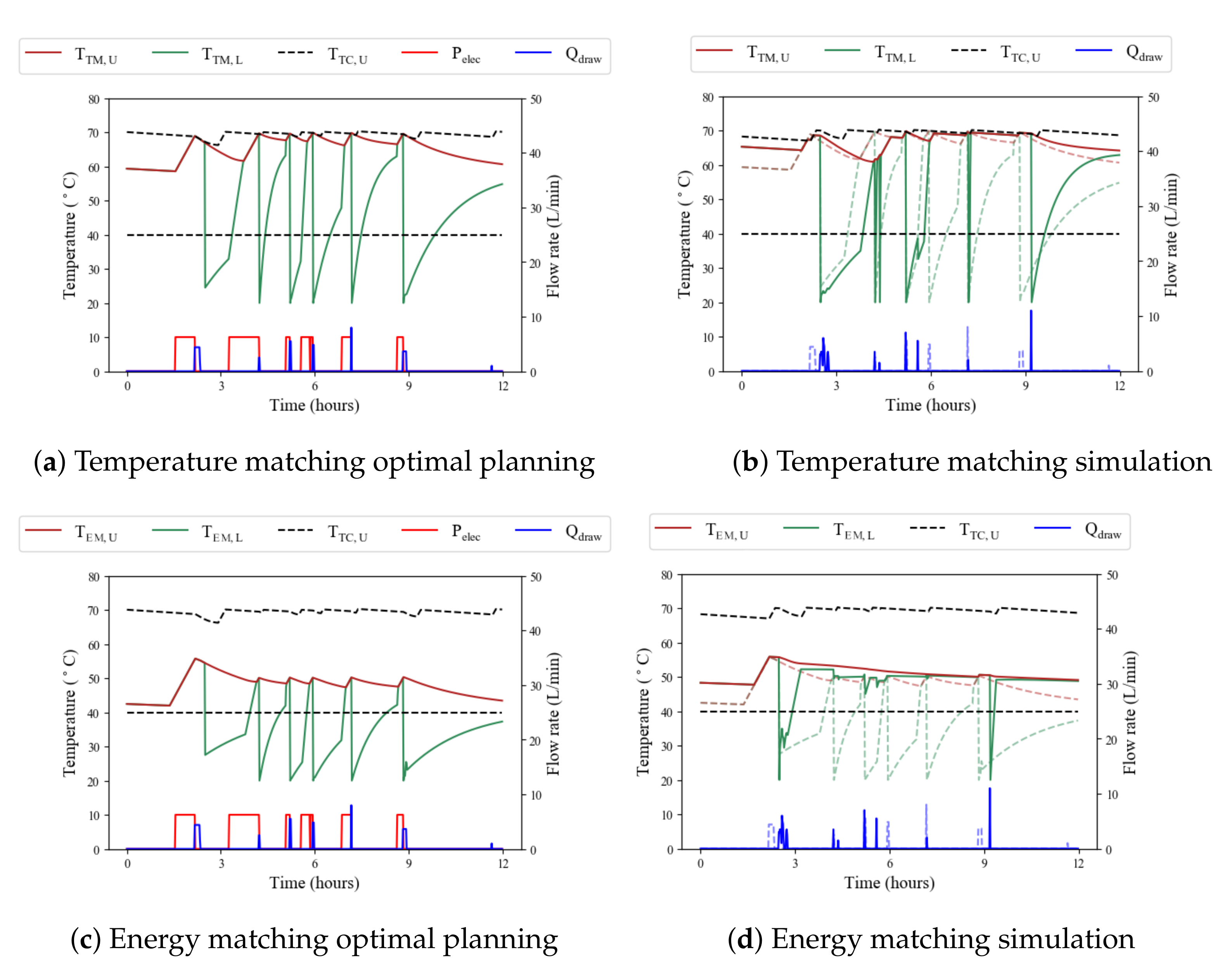
5.2. Simulation Results for an Individual EWH Using Predicted Hot Water Profiles

Figure 5 shows simulation results for an identical EWH for the TC, TM and EM control strategies for an arbitrary day in Summer. Each figure plots the upper and lower node temperature (represented by solid lines), outlet pipe flow rate $Q_{\mathrm{draw}}$ and the power supplied by the heating element $P_{\mathrm{elec}}$ (any non-zero value represents the element power rating) over duration of 12 h. Although all the simulations start at the same initial EWH temperature of 68.5 ${}^{\circ }\mathrm{C}$, the figures may not as they are captured at a later stage of the simulation. The optimal planning is first produced for predicted water usages and the EWH simulates it on the actual hot water usages. Figure 5a,c show the optimal heating schedule and temperature trajectory for a predicted water usage profile for TM and EM, respectively. Figure 5b,d show the corresponding simulated EWH temperatures for the actual water usages (solid line temperatures and water events) as a result of the temperature feedback controller which try to guide the simulation along the optimal plan for the predicted water usages and the water mixer (dashed line temperatures and water events). All the figures show the upper node temperature for TC (dashed black line), which is simulated for the predicted water profile in (a) and (c) and the actual water profile in (b) and (d).

Thermostat control (TC): Looking at the dashed temperature trajectory in Figure 5a, this strategy keeps the temperature at the 68.5 ${}^{\circ }\mathrm{C}$ set point temperature and fluctuates with 1.5 ${}^{\circ }\mathrm{C}$ hysteresis. When the first water usage occurs, the upper node temperature is observed to drop to 66 ${}^{\circ }\mathrm{C}$ due to water stratification that occurs between the hot upper node body of water and the cold inlet water entering the tank and forming the lower node. At this point, the heating element is switched on to raise the temperature back to the set-point temperature.

Optimal temperature matching (TM): In Figure 5a, it can be seen that the temperature of the optimal plan is equivalent to that of TC at the start of each water usage. Before the first usage at $t=3$, the EWH is in a one-node state because there is only an upper node temperature shown. When the water flow rate transitions to a non-zero value, the water in the tank splits into two nodes and the lower node temperature is at the temperature of the cold water entering through the inlet pipe. At this point, water stratification between the two nodes causes the lower node temperature to increase and the upper node temperature to decrease until they reach a common temperature and transition back to a one-node state. In Figure 5b, a comparison can be seen between the temperatures of the optimal plan for the predicted water usages (dashes lines) and those of the actual water profile used for the EWH simulation (solid lines). Since the predicted water usages are conservative, they ensure that a sufficient amount of energy is in the tank in preparation for the actual water usage event (even if it does not occur).

Optimal energy matching (EM): Figure 5c,d show similar behaviour to the previous strategy with the exception that the initial temperature of the water usage does not need to be equal to that of TC. Instead, the flow rate will adjust to ensure that an equivalent amount of thermal energy is delivered. If the optimal plan had perfect foreknowledge of the water usages, it would only need to prevent the temperature from dropping below 40 ${}^{\circ }\mathrm{C}$ during the usage. Since they are predicted, Figure 5c shows that the optimal plan ensures that the upper node temperature does not fall below 50 ${}^{\circ }\mathrm{C}$ during water usages, as a result of implementing the 10 ${}^{\circ }\mathrm{C}$ safety margin.

Optimal energy matching with Legionella prevention (EML): Although EML control is not shown in the plots, it produces similar results to EM except for the tank heating to 60 ${}^{\circ }\mathrm{C}$ at the largest predicted water usage of each day.

5.3. Metrics for Evaluating the Results of the EWH Model

The term event refers to a single water usage where a sequence of positive water flow samples are encapsulated by ones that are zero. This provides the convenience of identifying water draw patterns in the profile and for keeping a tally of the number of times that water is drawn from the EWH. A cold event refers to a water usage where the initial temperature is below the desired usage temperature of 40 ${}^{\circ }\mathrm{C}$. This provides a metric that counts the occurrence of water usages that inconveniences the user’s comfort.

A distinction is made between water usages that are intended and those that are unintentional. This is explained by water that leaves the tank and remains in the piping that connects the EWH to the end-use device without being effectively used. The reason for this can relate to the user accidentally opening the hot water tap when cold water was intended or opening a mixer tap somewhere between hot and cold. A water event that uses less than 2 $\mathrm{L}$ is considered unintentional (assuming that the diameter and length of a standard pipe is respectively 22 mm and 5 m) and is excluded from events. The optimisation algorithm will ignore imposing constraints that ensure the tank is heated sufficiently for unintentional water usages.

The performance of the EWH simulations for each strategy are firstly measured by the electrical energy supplied by the heating element $E_{elec}$, the thermal energy of the water that is drawn from the tank, intentionally and unintentionally, $E_{draw}$, and the energy lost from the tank to the environment, $E_{loss}$. These quantities are calculated as daily averages and are respectively calculated using

$${\overline{P}}_{\mathrm{elec}|i}=\frac{{\sum }_{k=1}^{N_h}{P}_{\mathrm{elec}|i}\left(k\right)\Delta t}{D}\mathrm{kWh}/\mathrm{day}$$

(24)

$${\overline{P}}_{\mathrm{draw}|i}=\frac{{\sum }_{k=1}^{N_h}{P}_{\mathrm{draw}|i}\left(k\right)\Delta t}{D}\mathrm{kWh}/\mathrm{day}$$

(25)

$${\overline{P}}_{\mathrm{loss}|i}=\frac{{\sum }_{k=1}^{N_h}{P}_{\mathrm{loss}|i}\left(k\right)\Delta t}{D}\mathrm{kWh}/\mathrm{day}$$

(26)

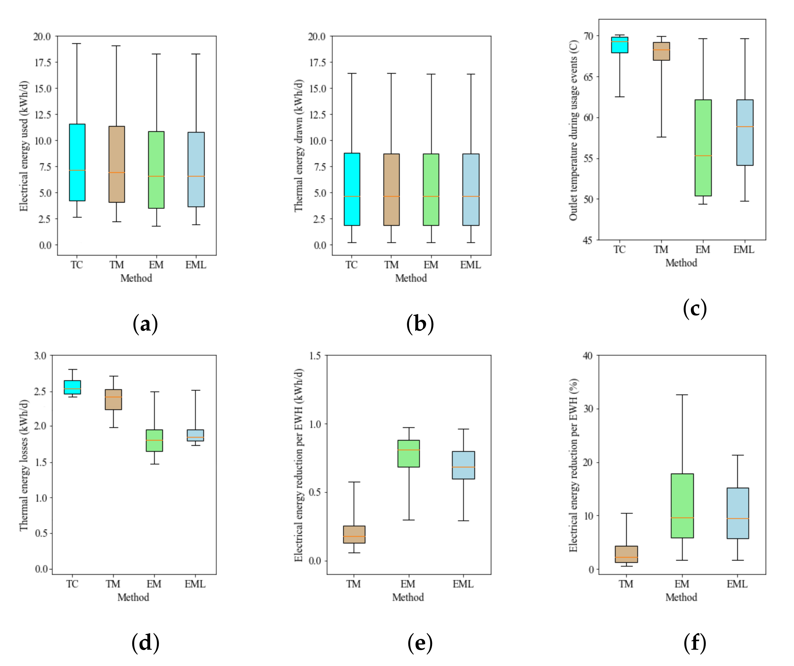
where i refers to an individual water heater, $\Delta t$ is the sampling period, $N_h$ and D are the total number of samples and days in the data set, and $P_{\mathrm{elec}|i}\left(k\right)$, $P_{\mathrm{elec}|i}\left(k\right)$ and $P_{\mathrm{elec}|i}\left(k\right)$ is the electrical power used, thermal energy used and thermal energy lost for heater i at time instant k. Another metric is defined that calculates the average water temperature during water usages and is represented as ${\overline{T}}_{usage}$. 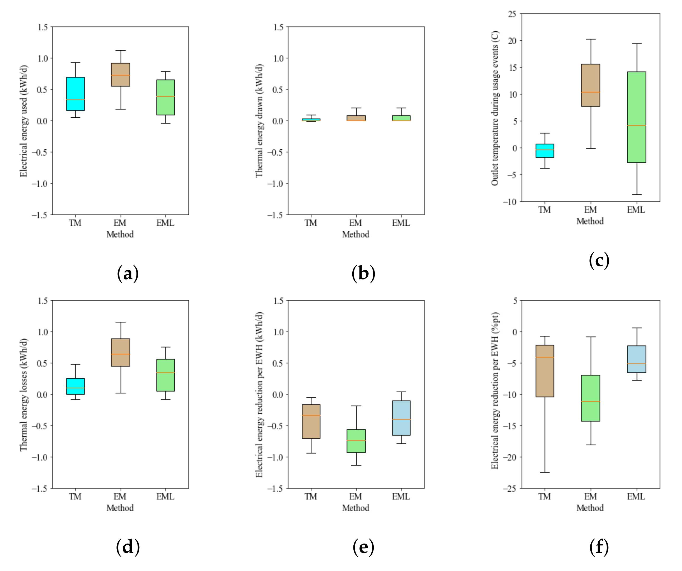The distributions for these results for TC, TM, EM and EML are shown in Figure 6a–d. Two metrics are calculated that evaluate the energy savings of the optimal control strategies relative to the baseline TC strategy. The reduction in electrical energy used per day by the optimal control strategies is expressed as kWh and as a percentage. For the TM strategy, they are calculated using

$$\Delta {\overline{P}}_{\mathrm{elec}|i,\mathrm{TM}}\left(\mathrm{kWh}/\mathrm{d}\right)={\overline{P}}_{\mathrm{elec}|i,\mathrm{TC}}-{\overline{P}}_{\mathrm{elec}|i,\mathrm{TM}}\mathrm{kWh}/\mathrm{day}$$

(27)

$$\Delta {\overline{P}}_{\mathrm{elec}|i,\mathrm{TM}}(\%)=\frac{{\overline{P}}_{\mathrm{elec}|i,\mathrm{TC}}-{\overline{P}}_{\mathrm{elec}|i,\mathrm{TM}}}{{\overline{P}}_{\mathrm{elec}|i,\mathrm{TC}}}\times 100\%$$

(28)

Figure 6e,f show the distribution of electrical energy savings for TM, EM and EML. Lastly, a metric is defined that counts the occurrence of cold events for an EWH simulation.

Table 2. Volume, energy, temperature and cold event results for two-node water heaters with planning based on predicted water usages.

		TC	TM	EM	EML
${\overline{V}}_{\mathrm{hot}}$	($\mathrm{L}/\mathrm{day}$)	119	123	150	142
$E_{\mathrm{elec}}$	($\mathrm{kWh}/\mathrm{day}$)	7.3	7.0	6.7	6.7
$E_{\mathrm{draw}}$	($\mathrm{kWh}/\mathrm{day}$)	4.7	4.7	4.7	4.7
$E_{\mathrm{loss}}$	($\mathrm{kWh}/\mathrm{day}$)	2.6	2.4	1.8	2.0
${\overline{T}}_{\mathrm{usage}}$	(${}^{\circ }\mathrm{C}$)	69.3	68.4	55.3	58.9
$\Delta E_{\mathrm{elec}}$(kWh)	($\mathrm{kWh}/\mathrm{day}$)	–	0.1, 0.2, 0.3	0.7, 0.8, 0.9	0.6, 0.7, 0.8
$\Delta E_{\mathrm{elec}}(\%)$	%	–	1.3, 2.2, 4.3	5.9, 9.6, 17.9	5.9, 9.6, 15.2
Cold events ${}^{*}$		0, 0, 0	0, 0, 0	0, 0, 0	0, 0, 0

Note: The distributions are represented as 25th percentile, median, 75th percentile. * Cold events are taken as the total cold events for the EWH that uses the 25th percentile, median, and 75th percentile of the total volume ofwater used.

statistically summarises the results for these metrics over all the EWH simulations.

5.4. Distribution of Results over All EWHs Using Two-Node Planning

The statistical results from all of the simulations performed for all 77 EWHs are discussed in this section. The results of each control strategy on temperature and energy for water heaters using a two-node model for optimal planning of predicted water usages are summarised in Table 2 and shown in Figure 6. Figure 6b shows that all the control strategies delivered the same amount of thermal energy as TC. This confirms that the water mixer was successful in adjusting the outlet flow rate for perfect energy matching for all the strategies. This reflects the fact that no matter which strategy is used, the user will adjust the hot water flow rate to receive the same energy for the same usage event.

5.4.1. Temperature-Matched Optimisation

Figure 6a shows that the median electrical energy used was $7.0$ kWh/day for TM, which is $0.3$ kWh/day ( $4.1$% ) less than the $7.3$ kWh/day median for TC. The median outlet temperature during events for TM dropped from $69.3$ ${}^{\circ }\mathrm{C}$ for TC to $68.4$ ${}^{\circ }\mathrm{C}$, as shown in Figure 6c. The difference is not significant, but it is caused by the lack of perfect temperature matching as a result of water usage predictions in the optimal planning. The temperature mismatching is also evident in the table, where the average volume of water drawn with TM increased to 123 $\mathrm{L}$ from the 119 $\mathrm{L}$ used with TC as a result of the mixer. Figure 6d indicates that the median thermal losses for TM was $2.4$ kWh/day ( $0.2$ kWh/day less than TC). Unlike the previous sections, the occurrence of cold events increased from that of TC. Although the increase was not serious, the number of cold events increased from 115 for TC to 141 for TM out of the 15,581 events. However, the additional cold events only occurred for EWHs that already had cold events: only five of the 77 EWHs had a cold event increase. The EWH with the biggest increase in cold events grew from 19 to 26 cold events of the 284 events (a 2.46% increase of the total events for the EWH). Looking at the distribution of savings in Figure 6e,f, the electrical energy reduction for TM was [0.1, 0.2, 0.3] $\mathrm{kWh}/\mathrm{day}$, or [1.3, 2.2, 4.3]% .

5.4.2. Energy-Matched Optimisation

The average outlet temperature gap between TC and EM is significantly smaller because of the 10 ${}^{\circ }\mathrm{C}$ safety margin imposed on the constraints. This explains why the outlet temperature does not drop below 50 ${}^{\circ }\mathrm{C}$ and the median outlet temperature for EM is $55.3$ ${}^{\circ }\mathrm{C}$. These increased outlet temperatures also cause the water mixer to adjust the outlet flow rate less to obtain the correct delivery of thermal energy. The average volume draw for EM is 150 $\mathrm{L}$, a substantial increase from 123 $\mathrm{L}$ of the previous section for EM when water usages were provided with perfect foreknowledge. The median electrical energy used was $6.7$ kWh/day for EM and, even though the electrical energy savings are reduced by the safety margins, a promising reduction in energy relative to TC is [0.69, 0.81, 0.88] $\mathrm{kWh}/\mathrm{day}$ and [5.9, 9.6, 17.9] % and the best savings is as much as 34.0%. These savings are attributed to the reduced median standing losses of $1.8$ kWh/day for EM which is $0.8$ kWh/day less than that of TC. The number of cold events increased from 115 of TC to 145, showing similar outcomes to TM with only four additional cold events.

5.4.3. Legionella Control

The results of EML show small differences from that of EM. This can be explained by the safety margin of 50 ${}^{\circ }\mathrm{C}$ which largely reduces the significance of the additional electrical energy required for the tank to reach 60 ${}^{\circ }\mathrm{C}$ each day. The median outlet temperature during usage increased to $58.9$ ${}^{\circ }\mathrm{C}$ for EML (a $3.6$ ${}^{\circ }\mathrm{C}$ increase from EM). The electrical energy used for EML is approximately equal to that for EM. The electrical energy reduction was [5.9, 9.6, 15.2]% and [0.6, 0.7, 0.8] $\mathrm{kWh}/\mathrm{day}$ relative to TC, where only the 75th percentile was different from EM. The occurrence of cold events for EML was equal to that of EM.

5.5. Metrics for Comparing Results of Optimal Planning without Accounting for Stratification

The effect of predicting water usages is determined by comparing the results that used the A* optimal planning which used perfect foreknowledge with the optimal planning that used predicted hot water usage profiles. The statistical results from all of the simulations performed for all 77 EWHs are discussed in this section. A metric is defined to assess the performance of the relative EWH-specific changes during the simulation. The average change in electrical energy used per day is calculated using

$${\overline{P}}_{\mathrm{elec}|h}^{\Delta N_p}={\overline{P}}_{\mathrm{elec}|h}^P-{\overline{P}}_{\mathrm{elec}|h}^A\mathrm{kWh}/\mathrm{day}$$

(29)

where the superscript $\Delta N_p$ refers to the difference between the types of planning and superscripts P and A refer to the simulation results that plan for predicted and actual water usage profiles, respectively. Similar modifications are applied to the formulas that calculate difference in thermal energy drawn per day, thermal energy losses per day, average outlet usage temperature during events and energy savings per day (kWh and percentage reduction). These results indicate the effect of predicting hot water usages when determining the optimal plan for an EWH. The simulation results for TM, EM and EML obtained in [42] for the optimal planning produced for a two-node EWH model with perfect foreknowledge of the water usages are compared with those obtained in Figure 6 for the optimal planning of predicted water usages.

5.6. Effects of Predicting Water Usages for Optimisation

Figure 7b shows that the median EWH delivered the same amount of thermal energy as TC for all the control strategies, with small deviations between the two types of planning, and shows that the mixer simulates the user drawing the same amount of thermal energy for each event, no matter the heating strategy used. Figure 7c shows that most of the outlet temperatures for TM with predicted water usage planning were perfectly matched to that of the results for simulations that had perfect water usage knowledge, which can also assume to be matched to TC. The small changes of the 25th and 75th percentiles of $2.0$${}^{\circ }\mathrm{C}$ and $0.8$ ${}^{\circ }\mathrm{C}$ respectively show the extent of the temperature mismatching to that of TC. For EM and EML, the median outlet temperature increases of $10.2$ ${}^{\circ }\mathrm{C}$ and $4.1$ ${}^{\circ }\mathrm{C}$, respectively, when water usages were predicted in the planning, show the impact of the safety margin is much harsher on EM. This is shown in Figure 7d where the median standing losses increase for EM and EML were $0.72$ kWh/day and $0.33$ kWh/day, respectively.

Figure 7a shows the median increase in electrical energy usage for TM, EM and EML were $0.35$ kWh/day (4.5%), $0.74$ kWh/day (19.6%) and $0.4$ kWh/day (11.6%), respectively, when planning is based on predicted water usages instead of perfect foreknowledge. This results in the final electrical energy saving decreases relative to TC which are shown in Figure 7e,f. The decreases in electrical energy savings due to the optimal planning using predicted water usages instead of perfect foreknowledge is [0.22, 0.31, 0.72] $\mathrm{kWh}/\mathrm{day}$, or [2.30, 4.11, 10.31] percentage points for TM; [0.57, 0.72, 0.90] $\mathrm{kWh}/\mathrm{day}$, or [7.1, 11.0, 14.0] percentage points for EM; and lastly, [0.09, 0.37, 0.65] $\mathrm{kWh}/\mathrm{day}$, or [2.33, 5.11, 6.31] percentage points for EML.

5.7. Discussion of the Effects of Predicting Hot Water Usages in the Planning

An evaluation of the results showed that the electrical energy usage increased for all the control strategies when the optimal planning is based on predicted water usages as opposed to perfect foreknowledge of the hot water profile. For TM, the median electrical energy savings decreased from 0.6 $\mathrm{kWh}/\mathrm{day}$ (6.3 percentage points) when perfect foreknowledge was used to 0.2 $\mathrm{kWh}/\mathrm{day}$ (2.2 percentage points) when predictions were used relative to the baseline TC strategy. This shows that TM does not save a lot when the water usage profile is predicted, as a result of safety measures which are implemented to minimise the risk of cold events. For EM and EML, the median electrical energy usage savings decreased from 1.6 $\mathrm{kWh}/\mathrm{day}$ (21.9 percentage points) and 1.2 $\mathrm{kWh}/\mathrm{day}$ (16.2 percentage points) when perfect foreknowledge was used to 0.8 $\mathrm{kWh}/\mathrm{day}$ (9.6 percentage points) and 0.7 $\mathrm{kWh}/\mathrm{day}$ (9.6 percentage points) when predictions were used. This ultimately shows that, even though there were huge energy saving reductions when the safety measures were imposed on the system, the energy matching strategies can still save close to 10 percentage points of electrical energy each day as well as preventing the growth of Legionella.

The number of cold events that occurred did increase for the three control strategies, however, of the total 15,581 events, the increase was 26 for TM and 30 for EM and EML. This result is not significant as they only occurred for five of the 77 EWHs and those EWHs already showed evidence of cold events occurring due to their heavy usages in TC. Because the outlet temperatures for TM did not deviate far from that of TC, it shows that these heavy water usage profiles were on the verge of having more cold events than what was counted. The results represent the practical savings that could be achieved. However, it should be noted that appropriate data acquisition and state estimation components would be required to estimate the internal states of the EWH for a real-world implementation.

6. Conclusions

The operation of a residential water heater requires a significant amount of electrical energy and raises concern for users in countries where electricity is purchased at a flat rate. Furthermore, the growing demand for electricity in these countries contributes to increased fossil fuels and the release of greenhouse gases. We determined how much energy can be saved practically by the optimal temperature planning of an EWH with stratification for 77 household’s water draw behaviour. The A* algorithm was implemented to produce the optimal heating schedule for three control strategies that were compared to a baseline strategy with the thermostat always on. The first ensured that water usages were temperature-matched to thermostat control, the second ensured that water usages were energy-matched to thermostat control at a lower temperature and larger volume, and the third was similar to the second but additionally ensured Legionella prevention. A probabilistic hot water usage model was used to predict water usages for the optimal heat scheduling which were simulated on actual water usage data. The outcome of the simulations showed that the median energy savings were 2.2% for TM and 9.6% for both EM and EML. Neither of the control strategies adversely increased the occurrence of cold events. Furthermore, optimal planning based on predicted water usages instead of perfect foreknowledge showed a median decrease in energy savings of 4.1 percentage points for TM, 11 percentage points for EM and 5.1 percentage points for EML. These results reflect the best energy savings that can be achieved with the optimal scheduling of an EWH without inconveniencing the user.

These practical energy savings could be be verified in further work by implementing the system in a real-world scenario and developing a means of communication between the physical EWH and the system’s software components. Furthermore, the system can be improved by providing varying ambient and inlet water temperature measurements based on real data.