Abstract
To ensure the safe operation of an interconnected power system, it is necessary to maintain the stability of the frequency and the tie-line exchanged power. This is one of the hottest issues in the power system field and is usually called load frequency control. To overcome the influences of load disturbances on multi-source power systems containing thermal power plants, hydropower plants, and gas turbine plants, we design a linear active disturbance rejection control (LADRC) based on the tie-line bias control mode. For LADRC, the parameter selection of the controller directly affects the response performance of the entire system, and it is usually not feasible to manually adjust parameters. Therefore, to obtain the optimal controller parameters, we use the Soft Actor-Critic algorithm in reinforcement learning to obtain the controller parameters in real time, and we design the reward function according to the needs of the power system. We carry out simulation experiments to verify the effectiveness of the proposed method. Compared with the results of other proportional–integral–derivative control techniques using optimization algorithms and LADRC with constant parameters, the proposed method shows significant advantages in terms of overshoot, undershoot, and settling time. In addition, by adding different disturbances to different areas of the multi-source power system, we demonstrate the robustness of the proposed control strategy.
1. Introduction
The interconnected power system has been developed in recent years to better meet power needs. To ensure the safe and reliable operation of the power system, the stability of the system’s frequency must be maintained. However, the mismatch between power generation and required power is prone to instability [1]. Therefore, load frequency control (LFC) and optimal power flow (OPF) [2] have become research hotspots in the field of multi-area interconnected power systems. The former mainly considers designing the controller to eliminate the influence of load disturbance on the frequency, and the latter determines the steady-state operating conditions containing the frequency distribution of the power system. In addition, there are multiple sources of power generation in power systems, among which thermal power generation, hydropower generation, and gas turbines are most common, and each has different characteristics. In this study, we mainly investigate the LFC of the multi-source power system.
For the LFC system in the non-deregulated environment, the control strategy needs to meet the performance requirements of frequency deviation and tie-line exchanged power at the planned value. Among various control strategies, proportional–integral–derivative (PID) control [3,4,5] occupies a dominant position inLFC due to its clear principle and simple implementation. However, PID is usually unsuitable for the demanding control requirements of LFC. Other control strategies such as robust control [6], model predictive control (MPC) [7], and adaptive control [8] could also achieve good results in LFC. For example, Zeng et al. [9] proposed an adaptive MPC method for a multi-area interconnected power system with PV generation realizing frequency deviation control. Rajeswari et al. [10] designed an adaptive LFC PID controller based on the generalized Hopfield neural network (GHNN), which can be used in situations where load demand is random, system dynamic modeling is inaccurate, the system model is nonlinear, and system parameter changes are uncertain. Although these methods can achieve higher control accuracy than PID, their design process is complex and they are challenging to implement in engineering applications. In reality, there may be multiple sources of power generation in one area. For example, Sahu [11] et al. applied the differential evolution (DE) optimized fuzzy PID to a two-area interconnected power system with multi-source power generation containing thermal plant, hydro plant, and gas turbine plant in a deregulated environment, which improved the dynamic performance.
Under these demands, active disturbance rejection control (ADRC) was proposed by Han [12]. It has a simple structure and does not rely on model information. At present, the most widely used ADRC is the linear ADRC (LADRC) [13], which linearizes the structure of the extended state observer (ESO) and nonlinear state error feedback (NLSEF) control law in ADRC. LADRC dramatically simplifies the design of the ADRC controller and significantly reduces the number of parameters that need to be adjusted, which greatly promotes the engineering application of ADRC. Currently, LADRC has been successfully applied in many fields, such as ship path following control [14], aircraft control [15], and hydraulic systems [16], to name a few. As for LFC, LADRC has also shown good control effects. For example, Tan et al. [17] applied LADRC to power systems with a deregulated environment to realize the stability of LFC. Tang et al. [18] studied the application of LADRC in the LFC of complex power systems with wind energy conversion systems and verified the effectiveness of the designed controller through simulations.
Although the number of controller parameters of LADRC has been greatly reduced compared with the original ADRC parameters, when the number of controllers increases, the determination of the parameters is still challenging. Therefore, parameter tuning is also a vital part of the controller design process. At present, the most widely studied parameter optimization methods are intelligent optimization algorithms, including particle swarm optimization (PSO) [19], genetic algorithm (GA) [20], and simulated annealing (SA) [21]. However, these algorithms have poor robustness and can only obtain the optimal parameters of the controller under certain operating conditions. Fuzzy control [22] can obtain adaptive parameter values depending on the model information. Neural networks [23] can obtain adaptive control parameters without relying on model information, but they do not cope well with sudden operating conditions. Therefore, an intelligent method that is robust and does not rely on models is urgently needed for tuning parameters.
Reinforcement learning [24] is an algorithm that simulates the decision-making process of the human brain, where the design of the reward function gives the algorithm its decision-making ability. The salient feature of reinforcement learning is to obtain reward feedback through interaction between the environment and the agent (brain) without knowing the environment’s information so as to realize the selection of the optimal action-value according to the environmental state. This realizes a process of self-adaptation in which action-values are selected according to the environmental state. With these advantages, reinforcement learning has achieved excellent results in path planning [25], games [26], and other fields. Recently, research has been conducted on reinforcement learning to adjust controller parameters. For example, Chen [27] and Zheng [28] applied Q learning to parameter tuning of LADRC. Nevertheless, Q learning is more suitable for systems with limited states and limited actions. Soft actor-critic (SAC) is an algorithm based on deep reinforcement learning that uses deep neural networks to remove the finite-dimensional restrictions on states and actions [29]. In addition, compared with the deep deterministic policy gradient (DDPG) algorithm, which is also suitable for continuous state and continuous action in reinforcement learning, the convergence of SAC is proved to be better. Therefore, in this study, we use SAC to solve the problem of LADRC parameters (continuous actions) tuning in LFC (continuous states).
In this study, based on a two-area interconnected power system with thermal power plants, hydropower plants, and gas turbine plants, we design three different LADRC methods for each area. Moreover, we use SAC to adjust the nine parameters of all controllers. The simulation results verify the effectiveness of the proposed method.
The rest of the paper is arranged as follows. Section 2 presents a model description of the two-area six-unit interconnected power system. Section 3 shows the design process of LADRC. Based on introducing SAC, Section 4 describes how SAC optimizes controller parameters. Section 5 demonstrates the superiority of the proposed method through simulation results. Section 6 concludes the paper.
2. Modeling of Two-Area Six-Unit Power System
We consider a two-area six-unit interconnected power system consisting of one thermal power plant, one hydropower plant, and one gas turbine plant in each area, as shown in Figure 1 [30], where each unit consists of a governor marked in light yellow and a turbine marked in light green. Moreover, the links marked in purple are generators . The symbols are defined in Table 1. Generally, the governor mainly controls the speed of the turbine, and the turbine converts mechanical energy into electrical energy. However, to ensure the safe and stable operation of the system, two conditions need to be met: one is that the frequency deviation is stable at 0, and the other is that the tie-line exchanged power is maintained at the planned value.
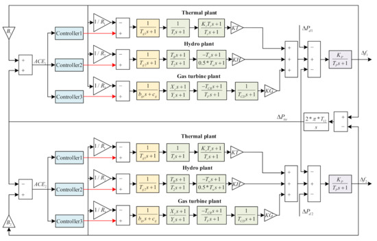
Figure 1.
Transfer function model of two-area six-unit power system.

Table 1.
Symbol definitions and values.
Then, from Figure 1, taking the first area as an example, the following derivation can be obtained:
where are the inputs of the three units, , , , , and .
where is expressed as
In addition, there are many uncertainties in the two-area six-unit power system, such as unmodeled dynamics, load disturbance, and internal parameter perturbations, which lead to model–reality mismatch. Therefore, our research goal in this study is to design controllers to make the system stable despite these uncertainties.
3. Design of LADRC
Because ADRC has a simple design, is model-free, and possesses self-decoupling characteristics, it has been favored by many scholars in recent years. In this study, we design an LADRC controller for the system shown in Figure 1. We adopt the tie-line bias control (TBC) [31] mode to simultaneously adjust the frequency deviation and the tie-line exchanged power, and we select as the controller input. As for the coupling of the system, we adopt a decentralized control method [32], that is, under the premise of ignoring the tie-line exchanged power, we design a controller for each area. As shown in Figure 1, the two areas have the same structure, so the two controllers will be identical.
The design of the LADRC does not require accurate model information of the system, only the order of the controlled plant. Let us take the first area as an example. Removing , we rearrange the expression of as
Then, for the thermal power unit, is the output of the first controller, and and are constants, that is,
Therefore, the system order of the thermal power unit is 3. Then, we can express the system as shown in Equation (6). In the same way, the system orders of the hydropower turbine unit and the gas turbine unit are 2 and 3, respectively. Therefore, taking the thermal power unit as an example, we design the LADRC as follows.
where f is the total disturbance, including the unmodeled dynamics, load disturbance, and parameter perturbation, and is an adjustable parameter. The core idea of LADRC is to estimate the total disturbance f through the linear extended state observer (LESO) and use the PD control combination to eliminate the disturbance.
We define the states as , , , and . Then, we design LESO as
where , , , and denote the estimated values of , , , and , respectively. Furthermore, , , , and represent the observer gains. We write the observer gain matrix as . Then, the suitable L can guarantee the accuracy of the estimation. For convenience, we configure the observer gain at the pole [33] using the pole configuration method as
Then,
In the case of , the disturbance is eliminated. Then, we can take in Equation (6) as
where
where , , and are the feedback control gains.
Finally, we rearrange Equation (6) into the following form, thereby realizing the compensation of disturbances:
Similarly, we configure the feedback control gain to the pole ,
Thus,
The structure diagram of LADRC is shown in Figure 2. The parameters that need to be adjusted in LADRC are , , and . Second order or third order linear active disturbance rejection controllers can be designed for the hydropower turbine unit and gas turbine unit following the above process. To sum up, the parameters that need to be adjusted are , , , , , , , , and .
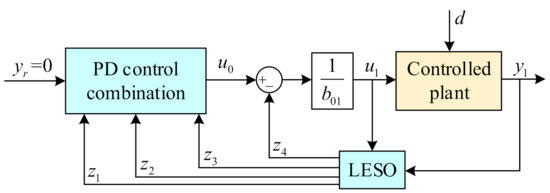
Figure 2.
Structure diagram of LADRC.
4. LADRC Parameter Optimization Based on SAC
Because it is challenging to adjust nine parameters at the same time manually, we use the SAC algorithm in reinforcement learning to adjust all controller parameters.
4.1. The Basics of SAC
Reinforcement learning is a method of solving sequential decision-making problems, and its process is usually expressed as a Markov decision process (MDP): . S and A represent the state space and action space, respectively, which need to be artificially defined. P is the probability of state transition, which represents the probability of transition from state and action to state , namely . R is the reward function, which reflects how close the actual state is to the target state. The goal of reinforcement learning is to find the optimal strategy through continuous iteration between the agent and the environment, that is, the probability of taking action a under the condition of state s: . Then, based on , the agent can choose the best action. In general, the state-action value function is used to evaluate the value of the action:
where is the cumulative reward (), and is the discount factor reflecting the the importance of the reward value in the future.
SAC is an algorithm in reinforcement learning that can solve continuous state space and continuous action space problems. The structure diagram of SAC is shown in Figure 3. It should be pointed out that, unlike Q in the traditional reinforcement learning algorithm, the Q value in SAC not only maximizes the cumulative reward but also increases entropy [34].
where represents the entropy under the policy , which is a measure that describe the uncertainty of random variables, , and is the weight of entropy.
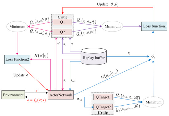
Figure 3.
Structure diagram of SAC.
It can be seen from Figure 3 that there are mainly three parts of SAC: the first is the replay buffer for storing data to train the networks, the second is the critic network used to generate the Q value, and the third is the actor network to generate the action value.
Four networks contain two Q networks and two target Q networks for the critic networks, where the target Q networks have the same structure as the Q networks. The addition of the target Q network improves the stability of network training. For example, assume that the corresponding weights of the four networks are , , , and , where the first two weights are updated through network training shown in Equation (17), and the latter two are updated through the exponential moving average method on the basis of and shown in Equation (19) [35], where is the target smooth factor.
where represents the Q network output when the network inputs are and and the network weight is . is expressed in Equation (18).
For the actor-network, its purpose is to generate the optimal action-value through the input of the state. In SAC, supposing that the weight of the actor-network is , the loss function is [34]
where is the Kullback–Leibler divergence and is the log partition function. Since has little effect on the update of the weight , it can be ignored, so Equation (20) can be rearranged as
The action can be obtained by the network input and the weight [36], which is expressed as
where is sampled from a Gaussian distribution, and and denote the mean value and covariance value of the network output.
4.2. The Design of Environment and the Agent
The main idea of SAC optimization is introduced above, and the optimal strategy is obtained by maximizing Q, that is, . The whole process is realized by the continuous interaction between the environment and the agent. In this study, the environment refers to the power system, including LADRC, and the agent is similar to the human brain and can make decisions. To optimize the parameters of LADRC, it is necessary to define the states, actions in the environment, and the reward function in the agent.
We define the state as follows:
where k is the simulation step.
The actions are the nine controller parameters to be optimized:
The reward function is the primary basis for how the agent reacts, so we establish the reward function according to the state. In this study, our control target is that the in the two areas can be stabilized to 0. Therefore, we give the reward function as
The whole process is shown in Figure 4, which mainly includes two stages. One is the training stage for training the connected critic networks and the actor-network, and the other is the online stage for using the trained actor-network to select parameters online.
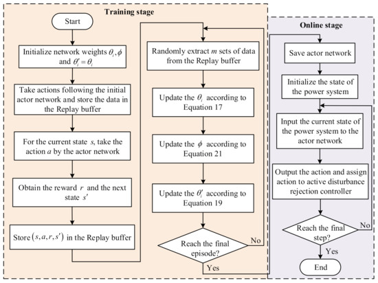
Figure 4.
Flowchart of LADRC parameter optimization based on SAC.
5. Simulation Results and Discussion
To verify the effectiveness of the proposed method, we conducted simulation experiments on the two-area six-unit interconnected power system shown in Figure 1. Table 2 shows the parameter settings during the SAC training process, where these parameters are chosen by multiple attempts, and Table 3 shows the optimization ranges of the nine parameters to be adjusted.
Table 2.
Parameter settings during SAC training.
Table 3.
Upper and lower bounds of controller parameters.
The critic network consists of a fully connected neural network with two hidden layers, in which the numbers of input and output neurons are 11 and 1, respectively, and the numbers of hidden layer neurons are 400 and 300, respectively. As for the actor-network, the structure is shown in Figure 5.
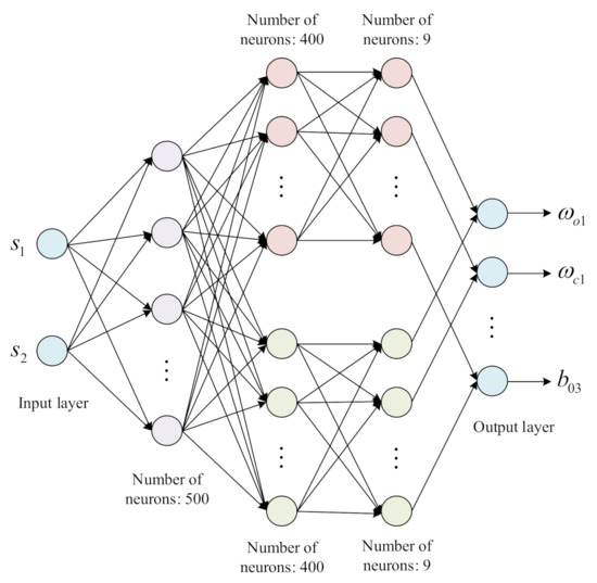
Figure 5.
Structure diagram of actor network.
In addition, to enable the proposed method to better cope with the impact of load disturbances, during the training process, we randomly add the step load disturbance of 0–0.03 p.u. to area 1 and area 2 in each iteration. We present the simulation verification results in the following subsection.
5.1. Performance Study of SAC-LADRC
Assuming that a load step disturbance of p.u. is added to the first area at t = 0, the response curve is shown in Figure 6, and the parameters optimized by SAC are shown in Figure 7, Figure 8 and Figure 9. To verify the effectiveness of the proposed method, Figure 7 also shows the control effect of the PID controller optimized by the differential evolution (DE) algorithm [37], the PID controller optimized by the hybrid stochastic fractal search and pattern search (hFSF-PS) algorithm [38], the PID controller optimized by the teaching learning based optimization (TLBO) algorithm [39], and the LADRC controller with conventional parameters. We select the parameters of LADRC as , , and . Table 4 shows the quantification results of performance indicators, including overshoot , undershoot , settling time , and integral of time-weighted absolute error () for frequency deviation and tie-line exchanged power. We calculate based on Equation (26).
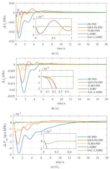
Figure 6.
Dynamic response comparison results.
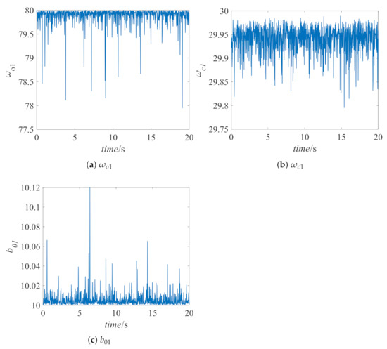
Figure 7.
Controller parameters of thermal power plant.
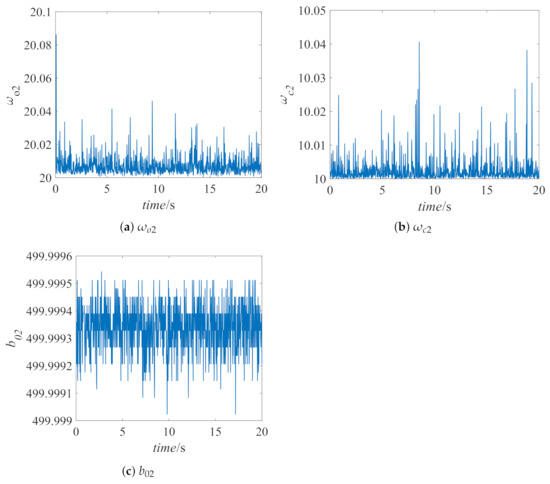
Figure 8.
Controller parameters of hydropower plant.
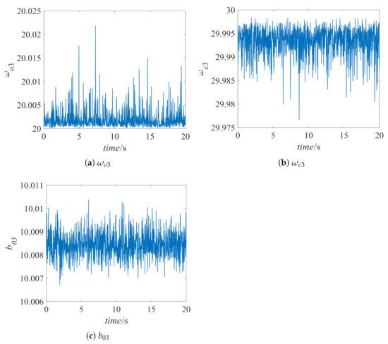
Figure 9.
Controller parameters of gas turbine plant.
Table 4.
Comparison of performance indicators of different control methods.
It can be seen from the partially enlarged view that the proposed method has obvious advantages in dynamic performance compared with other control methods, that is, the performance of SAC-LADRC has the smallest overshoot and the shortest response time. Furthermore, since the output of the actor-network is a distribution of parameters, the parameter results obtained by the proposed method will fluctuate in a small range, which is different from other reinforcement learning algorithms like Q learning, which will obtain stable parameter values when the system is stable.
5.2. Robustness Test of SAC-LADRC
To show the ability of the proposed method to suppress different load disturbances, we add the step load disturbance of p.u. to the first area at t = 0 s, the step load disturbance of p.u. to the first area at t = 10 s, and the step load disturbances of p.u. and p.u. to the second area at t = 20 s. The simulation results of the above-mentioned trained actor-network are shown in Figure 10.
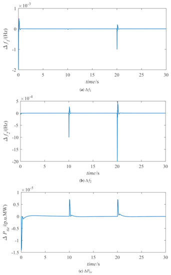
Figure 10.
Dynamic response with different disturbances.
It can be seen from Figure 10 that, despite the existence of various disturbances, the proposed method can still overcome the influence of load disturbances so that the frequency deviation and tie-line exchanged power quickly stabilize to 0.
6. Conclusions
We studied the LFC problem for a two-area interconnected power system with thermal power plants, hydropower plants, and gas turbine plants. Because traditional PID controllers are unable to meet the system’s high-efficiency operation requirements, we designed LADRC according to the characteristics of different power supplies. To further improve the control performance of LADRC, we used SAC for adaptive adjustment of multiple parameters. To be specific, according to the requirements of the LFC system, we designed the reward function based on the area control error (ACE). Compared with other methods such as DE-PID, hSFS-PS-PID, TLBO-PID, and traditional LADRC, the proposed method dramatically improves dynamic performance, including overshoot, undershoot, and settling time. Moreover, the response curves obtained by the trained agent under the influence of different step load disturbances show that the proposed method has good robustness. Generally speaking, the proposed method has the advantages of small error, short stabilization time, and good robustness, so it is an effective method to solve the LFC problem.
In future work, we will consider the application of the SAC algorithm in OPF [40,41]. Moreover, the high proportion of renewable energy is a development trend of the current power system. However, the large-scale grid connection of intermittent renewable energy represented by wind power and photovoltaics has brought challenges to the operation of the power system. Thus, the power system containing the renewable energies will be a focus of our research.
Author Contributions
Conceptualization, Y.Z. and Z.C.; methodology, J.T.; software, Y.Z.; validation, Y.Z. and Q.S.; formal analysis, Y.Z.; investigation, H.S.; resources, H.S.; data curation, Y.Z.; writing—original draft preparation, Y.Z.; writing—review and editing, J.T. and Q.Z.; visualization, M.D.; supervision, Q.S. and J.T.; project administration, J.T.; funding acquisition, J.T. All authors have read and agreed to the published version of the manuscript.
Funding
This work was supported by the National Natural Science Foundation of China (Grant No. 61973172, 61973175, 62003175 and 62003177), the National Key Research and Development Project (Grant No. 2019YFC1510900), and the key Technologies Research and Development Program of Tianjin (Grant No. 19JCZDJC32800). This project was also funded by the China Postdoctoral Science Foundation (Grant No. 2020M670633) and the Academy of Finland (Grant No. 315660).
Conflicts of Interest
The authors declare no conflict of interest.
References
- Arya, Y.; Dahiya, P.; Celik, E.; Sharma, G.; Gozde, H.; Nasiruddin, I. AGC performance amelioration in multi-area interconnected thermal and thermal-hydro-gas power systems using a novel controller. Eng. Sci. Technol. Int. J. 2021, 24, 384–396. [Google Scholar] [CrossRef]
- Tostado-Veliz, M.; Kamel, S.; Jurado, F. A Robust Power Flow Algorithm Based on Bulirsch–Stoer Method. IEEE Trans. Power Syst. 2019, 34, 3081–3089. [Google Scholar] [CrossRef]
- Tan, W. Unified tuning of PID load frequency controller for power systems via IMC. IEEE Trans. Power Syst. 2010, 25, 341–350. [Google Scholar] [CrossRef]
- Magdy, G.; Shabib, G.; Elbaset, A.A.; Mitani, Y. Optimized coordinated control of LFC and SMES to enhance frequency stability of a real multi-source power system considering high renewable energy penetration. Prot. Control. Mod. Power Syst. 2018, 3, 39. [Google Scholar] [CrossRef] [Green Version]
- Sahu, B.K.; Pati, T.K.; Nayak, J.R.; Panda, S.; Kar, S.K. A novel hybrid LUS-TLBO optimized fuzzy-PID controller for load frequency control of multi-source power system. Int. J. Electr. Power Energy Syst. 2016, 74, 58–69. [Google Scholar] [CrossRef]
- Tan, W.; Xu, Z. Robust analysis and design of load frequency controller for power systems. Electr. Power Syst. Res. 2008, 79, 846–853. [Google Scholar] [CrossRef]
- Liu, J.; Yao, Q.; Hu, Y. Model predictive control for load frequency of hybrid power system with wind power and thermal power. Energy 2019, 172, 555–565. [Google Scholar] [CrossRef]
- Fernandez-Guillamon, A.; Martinez-Lucas, G.; Molina-Garcia, A.; Sarasua, J.I. An adaptive control scheme for variable speed wind turbines providing frequency regulation in isolated power systems with thermal generation. Energies 2020, 13, 3369. [Google Scholar] [CrossRef]
- Zeng, G.; Xie, X.; Chen, M. An adaptive model predictive load frequency control method for multi-area interconnected power systems with photovoltaic generations. Energies 2017, 10, 1840. [Google Scholar] [CrossRef] [Green Version]
- Rajeswari, R.; Balasubramonian, M.; Veerapandiyan, V.; Loheswaran, S. Load frequency control of a dynamic interconnected power system using generalised Hopfield neural network based self-adaptive PID controller. IET Gener. Transm. Distrib. 2018, 12, 5713–5722. [Google Scholar]
- Sahu, K.S.; Sekhar, G.T.; Panda, S. DE optimized fuzzy PID controller with derivative filter for LFC of multi source power system in deregulated environment. Ain Shams Eng. J. 2015, 6, 511–530. [Google Scholar] [CrossRef] [Green Version]
- Han, J. Auto-disturbance-rejection controller and its applications. Control. Decis. 1998, 13, 19–23. [Google Scholar]
- Gao, Z. On the centrality of disturbance rejection in automatic control. ISA Trans. 2004, 53, 850–857. [Google Scholar] [CrossRef] [PubMed] [Green Version]
- Tao, J.; Du, L.; Dehmer, M.; Wen, Y.; Xie, G.; Zhou, Q. Path following control for towing system of cylindrical drilling platform in presence of disturbances and uncertainties. ISA Trans. 2019, 95, 185–193. [Google Scholar] [CrossRef]
- Sun, H.; Sun, Q.; Wu, W.; Chen, Z.; Tao, J. Altitude control for flexible wing unmanned aerial vehicle based on active disturbance rejection control and feedforward compensation. Int. J. Robust Nonlinear Control. 2020, 30, 222–245. [Google Scholar] [CrossRef]
- Jiang, Y.; Sun, Q.; Zhang, X.; Chen, Z. Pressure regulation for oxygen mask based on active disturbance rejection control. IEEE Trans. Ind. Electron. 2017, 64, 6402–6411. [Google Scholar] [CrossRef]
- Tan, W.; Hao, Y.; Li, D. Load frequency control in deregulated environments via active disturbance rejection. Int. J. Electr. Power Energy Syst. 2015, 66, 166–177. [Google Scholar] [CrossRef]
- Tang, Y.; Bai, Y.; Huang, C.; Du, B. Linear active disturbance rejection-based load frequency control concerning high penetration of wind energy. Energy Convers. Manag. 2015, 95, 259–271. [Google Scholar] [CrossRef]
- Grisales-Norena, L.F.; Montaoya, D.G.; Ramos-Paja, C.A. Optimal sizing and location of distributed generators based on PBIL and PSO techniques. Energies 2018, 11, 1018. [Google Scholar] [CrossRef] [Green Version]
- Assareh, E.; Behrang, M.A.; Assari, M.R.; Ghanbarzadeh, A. Application of PSO (particle swarm optimization) and GA (genetic algorithm) techniques on demand estimation of oil in Iran. Energy 2010, 35, 5223–5229. [Google Scholar] [CrossRef]
- Yang, K.; Cho, K. Simulated annealing algorithm for wind farm layout optimization: A benchmark study. Energies 2019, 12, 4403. [Google Scholar] [CrossRef] [Green Version]
- Feng, Y.; Wu, M.; Chen, X.; Chen, L.; Du, S. A fuzzy PID controller with nonlinear compensation term for mold level of continuous casting process. Inf. Sci. 2020, 539, 487–503. [Google Scholar] [CrossRef]
- Kang, J.; Meng, W.; Abraharn, A.; Liu, H. An adaptive PID neural network for complex nonlinear system control. Neurocomputing 2014, 135, 79–85. [Google Scholar] [CrossRef]
- Arulkumaran, K.; Deisenroth, M.P.; Brundage, M.; Bharath, A.A. Deep reinforcement learning: A brief survey. IEEE Signal Process. Mag. 2017, 34, 26–38. [Google Scholar] [CrossRef] [Green Version]
- Zhao, Y.; Qi, X.; Ma, Y.; Li, Z.; Malekian, R.; Sotelo, M.A. Path following optimization for an underactuated USV using smoothly-convergent deep reinforcement learning. IEEE Trans. Intell. Transp. Syst. 2020, 1–13. [Google Scholar] [CrossRef]
- Lu, M.; Li, X. Deep reinforcement learning policy in Hex game system. In Proceedings of the 2018 IEEE Chinese Control and Decision Conference (CCDC), Shenyang, China, 9–11 June 2018. [Google Scholar]
- Chen, Z.; Qin, B.; Sun, M.; Sun, Q. Q-Learning-based parameters adaptive algorithm for active disturbance rejection control and its application to ship course control. Neurocomputing 2019, 408, 51–63. [Google Scholar] [CrossRef]
- Zheng, Y.; Chen, Z.; Huang, Z.; Sun, M.; Sun, Q. Active disturbance rejection control for multi-area interconnected power system based on reinforcement learning. Neurocomputing 2021, 425, 149–159. [Google Scholar] [CrossRef]
- Haarnoja, T.; Zhou, A.; Abbeel, P.; Levine, S. Soft Actor-Critic: Off-policy maximum entropy deep reinforcement learning with a stochastic actor. In Proceedings of the 35th International Conference on Machine Learning, Stockholm, Sweden, 10–15 July 2018. [Google Scholar]
- Huang, Z.; Chen, Z.; Zheng, Y.; Sun, M.; Sun, Q. Optimal design of load frequency active disturbance rejection control via double-chains quantum genetic algorithm. Neural Comput. Appl. 2021, 33, 3325–3345. [Google Scholar] [CrossRef]
- Kang, Y. Research of Load Frequency Control for Multi-Area Interconnected Power System. Master’s Thesis, Northeastern University, Sheyang, China, 2015. [Google Scholar]
- Tan, W. Tuning of PID load frequency controller for power systems. Energy Convers. Manag. 2009, 50, 1465–1472. [Google Scholar] [CrossRef]
- Gao, Z. Active disturbance rejection control: A paradigm shift in feedback control system design. In Proceedings of the 2006 American Control Conference, Minneapolis, MN, USA, 14–16 June 2006. [Google Scholar]
- Haarnoja, T.; Zhou, A.; Hartikaninen, K.; Tucker, G.; Ha, S.; Tan, J.; Kumar, V.; Zhu, H.; Gupta, A.; Abbeel, P.; et al. Soft actor-critic algorithms and applications. arXiv 2018, arXiv:1812.05905. [Google Scholar]
- Fu, F.; Kang, Y.; Zhang, Z.; Yu, F.R.; Wu, T. Soft actor-critic DRL for live transcoding and streaming in vehicular fog-computing-enabled IoV. IEEE Trans. Things J. 2021, 8, 1308–1321. [Google Scholar]
- Duan, J.; Guan, Y.; Li, S.E.; Ren, Y.; Sun, Q.; Cheng, B. Distributional soft actor-critic: Off-policy reinforcement learning for addressing value estimation errors. IEEE Trans. Neural Netw. Learn. Syst. 2021, 1–15. [Google Scholar] [CrossRef]
- Mohanty, B.; Panda, S.; Hota, P.K. Controller parameters tuning of differential evolution algorithm and its application to load frequency control of multi-source power system. Electr. Power Energy Syst. 2014, 54, 77–85. [Google Scholar] [CrossRef]
- Padhy, S.; Panda, S. A hybrid stochastic fractal search and pattern search technique based cascade PI-PD controller for automatic generation control of multi-source power systems in presence of plug in electric vehicles. CAAI Trans. Intell. Technol. 2017, 2, 12–25. [Google Scholar] [CrossRef]
- Barisal, A.K. Comparative performance analysis of teaching learning based optimization for automatic load frequency control of multi-source power systems. Electr. Power Energy Syst. 2015, 66, 67–77. [Google Scholar] [CrossRef]
- Swief, R.A.; Hassan, N.M.; Hassan, H.M.; Abdelaziz, A.Y.; Kamh, M.Z. Multi-regional optimal power flow using marine predators algorithm considering load and generation variability. IEEE Access 2021, 9, 74600–74613. [Google Scholar] [CrossRef]
- Swief, R.A.; Hassan, N.M.; Hassan, H.M.; Abdelaziz, A.Y.; Kamh, M.Z. AC&DC optimal power flow incorporating centralized/decentralized multi-region grid control employing the whale algorithm. Ain Shams Eng. J. 2021, 12, 1907–1922. [Google Scholar]
Publisher’s Note: MDPI stays neutral with regard to jurisdictional claims in published maps and institutional affiliations. |
© 2021 by the authors. Licensee MDPI, Basel, Switzerland. This article is an open access article distributed under the terms and conditions of the Creative Commons Attribution (CC BY) license (https://creativecommons.org/licenses/by/4.0/).