Article

A Novel Optimization Algorithm for Solar Panels Selection towards a Self-Powered EV Parking Lot and Its Impact on the Distribution System

1
Canada Excellence Research Chair Team, Concordia University, Montreal, QC H3G 1M8, Canada
2
Department of Electrical Engineering, Faculty of Technology, University of Batna 2, Fesdis 05078, Batna, Algeria
*
Author to whom correspondence should be addressed.
Energies 2021, 14(15), 4515; https://doi.org/10.3390/en14154515
Submission received: 20 May 2021 / Revised: 16 July 2021 / Accepted: 19 July 2021 / Published: 26 July 2021
(This article belongs to the Special Issue Community Microgrids)

Abstract

:
This paper proposes an original multi-criteria decision-making optimization algorithm to select the best solar panels in an existing market and optimally size the photovoltaic (PV) system for an electric vehicle parking lot (EVPL). Our proposed algorithm is called rank-weigh-rank (RWR), and it is compared to the well-known technique for order of preference by similarity to ideal solution (TOPSIS) optimization algorithm under the same conditions for validation purposes. Results show that the speed of our proposed algorithm (RWR) in finding the best solution increases exponentially compared to TOPSIS when the numbers of alternatives and criteria increase. Moreover, 77% is the probability of obtaining results with more than 80% accuracy compared to TOPSIS, which validates the efficiency of our algorithm. In addition, we were able to design an EVPL with a power self-sufficiency ratio of 60.8%, the energy self-sufficiency ratio of 74.7%, and a payback period of 10.58 years. Moreover, the renewable energy-based EVPL was able to reduce the power losses on the network by 95.7% compared to an EVPL without a renewable energy system and improve the voltage deviation.

1. Introduction

1.1. Motivation and Background

Nowadays, there is a transition in the transportation sector from conventional cars to electric vehicles (EVs) to reduce the carbon footprint [1], and reach the target of zero-carbon emission in societies and cities [2,3]. The transition from conventional cars to EVs implies a transition from a conventional electrical network to a smarter grid [4], which necessitates changes in the electrical and transportation infrastructures. The deployment of EVs in cities and districts has to be accompanied by an expansion of the electrical infrastructure in which new charging stations and parking lots must be built to facilitate the deployment of EVs [5]. However, EVs have large batteries that consume lots of energy during a short period. Hence, they can increase the stress on the electrical network, especially in electric vehicle parking lots (EVPLs) and charging stations, which will increase the technical and financial losses in the distribution system [5,6]. In the presence of thousands of different solar panels (SPs) in the market, it becomes challenging to choose the best alternative for a particular application [7]. For instance, do we select SPs with the highest power generation, the highest efficiency, or the less expensive ones? Does a costly photovoltaic (PV) system produce more energy compared to a cheaper one? Many questions can be asked in which the answer seems not to be possible without using advanced optimal selection tools such as multi-criteria decision-making (MCDM) methods.

1.2. Literature Review

The deployment of renewable energy systems (RESs) has been extensively studied in the last decade [8,9,10,11]. The selection of the RES and its appropriate technologies depend on the location and the size of the project. For a particular RES such as photovoltaics, the market is overwhelmed with different solar panels, which have a wide variety of photovoltaic cell technologies, specifications, and dimensions (e.g., length, width, and thickness). The most important factors to take into consideration when selecting solar panels are the dimension of the SP (short and long lengths, and total area of the panel), cost, efficiency, power rating under standard test conditions (STC), warranty, brand name, quality, technology (e.g., monocrystalline, polycrystalline cells, and thin-film) [12], etc. Also, other external factors play an important role in selecting the best SPs, such as weather data (i.e., ambient temperature, solar irradiance, wind speed), dimensions of the rooftop or the area where the SPs will be installed, energy demand of the consumer, the payback period, the electricity tariff, and many others. Given this, it is complex to select the best solar panels without using a sophisticated algorithm, especially with the existence of hundreds of thousands of different solar panels in the market from many manufacturers.
The integration of PVs in parking lots has become of high interest to many researchers in recent years. Some papers, such as [13], studied the optimal size and siting of hybrid renewable energy sources, including PV, wind turbines, and diesel generators. Based on this distributed generation’s optimal sizing and siting, the authors proposed building a movie theater complex with a plug-in hybrid electric vehicle parking lot. Despite using the genetic algorithm to solve the problem, and despite the authors being able to reduce the power loss and improve the voltage profile, the study is not realistic since buildings are built anywhere without even considering what their impact will be on the distribution network. Moreover, the paper did not consider the availability of many solar panel technologies and their specifications in the market. The optimal charging scheduling of EVs in a workplace parking lot in the presence of a PV power system was studied in [14]. The paper did not study the optimal sizing of the PV system nor the SPs’ optimal selection from a list in the existing market. On the other hand, paper [15] studied the impact of an EVPL on the distribution network with and without roof-mounted PV systems. Results were impressive in which the integration of SPs in the EVPL lot reduced the power loss; it also reduced the stress on the network and the voltage deviation. However, the main drawback of this paper is that it did not study the impact of considering different solar panels on the network. The authors in [16] proposed a heuristic optimization algorithm to optimally size a hybrid PV-battery-diesel energy system on the network considering an EVPL with bidirectional power flow from the EVs. It was shown that the discharging mode of the EVs can reduce the total cost of the optimal sizing of system by almost 5.2%. Authors optimally sized the hybrid system without selecting the best alternatives from existing lists in the market.
Multi-Criteria Decision Making (MCDM) methods are mostly used to rank and select the best option from a list of alternatives considering different criteria and weighting factors. MCDM is widely used in all domains such as waste management, energy, economics, transportation, planning, etc. [17]. According to [17], the most common MCDM methods are: (i) technique for order of preference by similarity to ideal solution (TOPSIS), (ii) simple additive weighting, (iii) Preference ranking organization method for enrichment evaluation (PROMETHEE), (iv) ÉLimination et Choix Traduisant la REalité (ELECTRE), (v) goal programming, (vi) multi-attribute utility theory (MAUT), (vii) simple multi-attribute rating technique, (viii) data envelopment analysis, (ix) case-based reasoning, (x) fuzzy set theory, and (xi) analytic hierarchy process. Many literature reviews compared different MCDM methods and presented their advantages and disadvantages and the fields where they are mostly applied, as in [16,18,19,20,21,22,23,24,25,26,27]. Sometimes, it is preferable to use certain methods in specific fields, while they are not recommended in others since each method has some advantages and disadvantages. For example, MAUT has been heavy used in agricultural, energy management, water management, actuarial, financial, and economic problems, while it is less recommended for projects or fields where there are less available input data, fewer preferences, and unprecise assumptions. Despite the fact that many papers studied the design and implementation of MCDM in different fields, there are very few that studied the optimal selection and ranking of solar panels from a list of alternatives using MCDM methods. These papers are listed hereafter. Paper [28] studied the optimal selection of SPs by using the analytical hierarchy process (AHP). The authors considered many criteria, including environmental, economic, mechanical, electrical, and customer requirements. The paper selected the best SP with a rated power of 200 W from only six alternatives, which is not considered enough for comparison. The paper presented a confusing interpretation of the results, especially when the authors said that the SPs with the highest efficiencies have the shortest payback periods (PBP). This interpretation is not accurate since the PBP depends on many factors that were not considered in the paper (such as energy consumption and generation, weather data, selling and buying electricity price, and the total installation cost of the system). A fuzzy MCDM was presented in [29] to select the best SP to design a PV power plant. Many constraints were considered, such as the supply capacity, product price, delay cost, quality cost, and others. However, the proposed approach did not consider many important factors that might affect the selection of the SPs, such as the consumers’ energy demand, the impact of the weather conditions on the output power of the PV system, and others. All these factors affect the PV output energy and may mislead the decision-maker to choose the best SP for a specific application. In reference [30], the authors compared different solar panel technologies and brands. Many economic and technical aspects are considered, such as cumulative cash flow, levelized cost of electricity, monthly efficiency of the PV modules, and annual electricity generation. The authors made a good comparison; however, they did not use any MCDM or optimization technique. Therefore, it became difficult to choose the best SP without using a sophisticated algorithm, especially when dealing with hundreds of thousands of different SPs. In [31], the authors considered that the selection of solar panels encompasses complex factors involving both quantifiable and subjective parameters, which should be balanced in order to select the solar panels appropriately. They proposed an integrated method by combining the fuzzy analytical hierarchy process and TOPSIS to select a 100 W solar panel. The authors considered a few criteria, which are not enough to select the best solar panels for the case of an EVPL. In our previous work [32], we developed an algorithm to optimally select the best solar panels from a list of alternatives for the case of a small home with low energy consumption. However, it was not known whether the method could be applied for a larger project such as an EVPL with high energy demand. To the best of our knowledge, MCDM is not used to select the best SP for the case of an EVPL. Moreover, it is unknown whether choosing the best or not the best SPs has any techno-economic impact on the distribution network. Also, the concept of a self-sufficient EVPL is not studied and needs further investigation.

1.3. Contribution

The main goal of this study is to design an EVPL that is able to generate its own energy need by installing a roof-mounted PV system considering many criteria and constraints. The contributions in this paper are stated as follows:
  • A rank-weigh-rank (RWR) optimization algorithm is proposed to rank and select the best solar panels from a list of alternatives. In addition, it optimally places and distributes the solar panels on the rooftops of the EVPL considering many criteria and constraints,
  • Some equations and definitions are proposed as presented in Algorithm 1, including but not limited to: energy and power self-sufficiency ratios, excess and lack of energy production ratio, surface filling ratio, etc.
For validation purposes, our proposed RWR optimization algorithm is compared to the well-known TOPSIS method regarding their accuracy, similarities, and speed in finding and ranking the best alternatives. A case study in Montreal was considered in which our goal was to design a roof-mounted PV system and select the best solar panels from an existing list. The impact of selecting or not selecting the best SPs on the voltage deviation and power losses of the distribution network was studied for three case scenarios as follows:
Case 1: EVPL without roof-mounted PV system;
Case 2: EVPL with roof-mounted PV System with the best selected SP using RWR method;
Case 3: EVPL with roof-mounted PV system without selecting the best SP.

2. Proposed Algorithm to Select the Best Solar Panel from a List

This section presents the proposed RWR optimization algorithm for selecting and ranking the best solar panels in a set of alternatives considering many criteria and constraints. The main goal is to maximize the self-sufficiency of the EVPL by installing only solar panels while minimizing the payback period. Algorithm 1 shows the steps to follow in order to select the best solar panel from a list and optimal size and distribute the panels on the rooftops of the EVPL. In the first section of the algorithm (steps 1 to 6), the algorithm collects real data from the weather, the historical power, and energy demand profiles of the EVPL, characteristics of the parking lot (e.g., number of chargers, charging rate (6 kWp @ level 2), arrival and departure time of EVs, opening hours, etc.), electricity tariffs, and existing solar panels in the market. In the second section (steps 7 to 20), the algorithm starts to calculate the necessary criteria and data which will be used to sort and select the best solar panels, and to design the roof-mounted PV system. To facilitate the visibility of the paper, all equations are left to Appendix A for more details. In the third section (steps 21 to 29), a decision matrix is created in which the most pertinent constraints and criteria will be used by the RWR optimization algorithm. These constraints and criteria are divided into two categories, beneficial (e.g., energy self-sufficiency ratio) and non-beneficial (e.g., payback period). In the last section (steps 30 to 33), the proposed RWR optimization algorithm is implemented in which it ranks the alternatives based on the weighting factors provided by the designer and the decision matrix. Finally (step 34), the algorithm selects the best alternative and suggests the optimal dimension and placement of the roof-mounted PV system.
Algorithm 1. Proposed algorithm for optimal selection and distribution of the solar panels for a roof-mounted photovoltaic (PV) system in an electric vehicle parking lot (EVPL).
Input Data
1Weather data: Solar irradiance, ambient temperature, wind speed
2Historical power profiles and energy demand of the EVPL
3Parking lot data, such as the maximum number of occupancies of EVs, charging rates (e.g., level 2, 6 kWp), arrival and departure time of each EV, opening and closing hours (e.g., from 8 a.m. till 11 p.m.),
4Buying and selling electricity prices for the following cases: Grid EV, RES→EV, RES→Grid
5Roof dimensions: number of roofs, their length, width, and inclination,
6Solar panel data:
a. Shape of the PV module: short and long side lengths and area, and tile angle
b. Spacing between solar panels, and between solar panels and the boundaries of the roofs,
c. Internal Characteristics of the solar panels: total installation cost per module, efficiency, geometric multiplier, temperature coefficients for the current and voltage, current and voltage rating, technology, PTC, MPPT, and many others as listed in Table 1
Calculate the following equations
DescriptionEquationsReferences
7Efficiency of the systemEquation (A1)[33]
8Number of modules in a rowEquation (A2)(New equation)
9Number of modules in a column Equation (A4)(New equation)
10Total number of modulesEquation (A5)(New equation derived from [33])
11Installed capacity of the PV systemEquation (A6)(New equation)
12Total installation cost of the PV systemEquation (A7)(New equation)
13Cost to power generation ratio  (CPR)Equation (A8)(New equation)
14Cost to energy generation ratio  (CER)Equation (A9)(New equation)
15Payback period (PBP)Equation (A12)(New equation)
16Output power & energy of the PV SystemEquations (A16) and (A17)(New equation derived from [33])
17Energy self-sufficiency ratioEquation (A18)[34]
18Power self-Sufficiency ratioEquation (A19) (New equation)
19Excess and lack of energy production ratioEquation (A20) and (A21)(New equation)
20Surface filling ratioEquation (A22)(New equation)
Create a decision matrix ( M i , j ) with the following criteria (where i [ 1 , I ] and j [ 1 , J ] are the i -th alternative, and the j -th criterion)
21MPPT under STCbeneficial criteria
22Total installation cost per modulenon-beneficial criteria
23Installed capacity of the PV systembeneficial criteria
24Total installation cost of the PV systemnon-beneficial criteria
25Cost to power generation rationon-beneficial criteria
26Cost to energy generation rationon-beneficial criteria
27Efficiency of the PV systembeneficial criteria
28Payback periodnon-beneficial criteria
29Energy self-sufficiency ratio beneficial criteria
Use Rank-Weigh-Rank (RWR) method to rank alternatives in the decision matrix (Our proposed MCDM algorithm)
30Rank the alternatives of each criterion from the best to the worst values N i , j = rank ( M i , j ) . The ranking can be in ascending order for the non-beneficial criteria (e.g., cost), and in descending order for the beneficial criteria (e.g., energy generation)
31Create a Weighting Vector which weighs criteria using the equation w j = W j j = 1 J W j , where W j [ 0 , 10 ]   j is the weighting factor for the j -th criterion, and w j is the normalized weighting factor, w j [ 0 , 1 ]   j
32Calculate the normalized weighted decision vector V i = M i , j · w j T . Where, w j T is the transposition of the vector w j ,
33 Rank the obtained vector V i in ascending order R i = rank ( V i , ascend )
Results
34Select the best alternative and calculate the optimal dimensioning and placement of the solar panels on the roofs of the EVPL

3. Assumptions and Considerations

To validate the proposed RWR optimization algorithm for ranking and selecting the best solar panels, it is necessary to clarify this paper’s context and framework. The RWR optimization algorithm is compared to the well-established TOPSIS method taking into account many criteria and constraints, and studying their speed in ranking the best alternatives, and their similarities in selecting the same best solutions. Since this paper deals with the design of an energy self-sufficiency EVPL with a roof-mounted PV system, it is important to study the technical impact of selecting different solar panels on the electrical distribution network regarding voltage stability and power losses. To do so, three different cases are considered:
  • Case 1: EVPLs without roof-mounted PV systems;
  • Case 2: EVPLs with roof-mounted PV systems while selecting the best solar panels using our proposed RWR optimization algorithm;
  • Case 3: EVPLs with roof-mounted PV system without using our proposed RWR optimization algorithm to select the best solar panels.
In this paper, a real case study is conducted in Montreal, Canada, using real data for 2019, as presented in the following subsections.

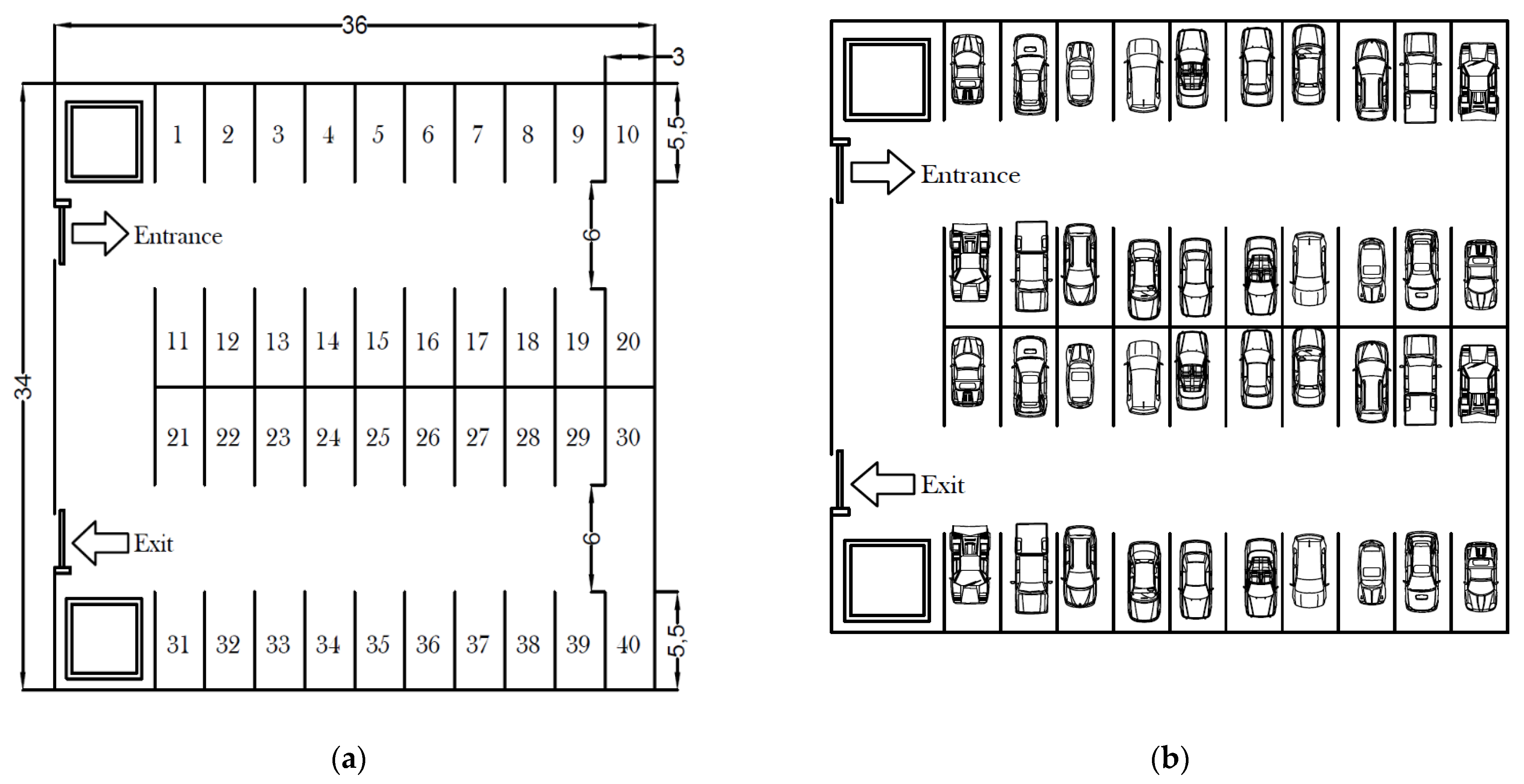
3.1. Electric Vehicle Parking Lot Data

Figure 1 shows a typical parking lot in Montreal, Canada. In this paper, we consider a parking lot for electric vehicles with the following specifications:
  • Parking lot is for a supermarket with an area of 1224 m2;
  • Opening hours from 8:00 a.m. till 11:00 p.m.;
  • AC Level 2 charger is used in which the power rate is variable between 0 and 6 kWp;
  • Maximum power capacity of the parking lot is 240 kWp;
  • Maximum number of EVs in the parking lot: 40;
  • Rate M is applied for the parking lot in Quebec:
    $14.58 per kilowatt of billing demand (EVPL will have a maximum of 240 kWp (6 kWp × 40 EVs). Therefore, the total rate is $3499.2 (240 kWp × 14.58 $/kW),
    Plus 5.03 ¢ per kWh for the first 210,000 kilowatt-hours per month,
    And 3.73 ¢ per kWh per month for the remaining consumption.
  • Selling electricity price:
    From PV to EV: 15 ¢/kWh,
    From PV to the grid: 5.03 ¢/kWh,
  • Since we are comparing different SPs, the price of the infrastructure is not included in the calculation because it will be the same for any kind of SPs, and it will not affect the output results.

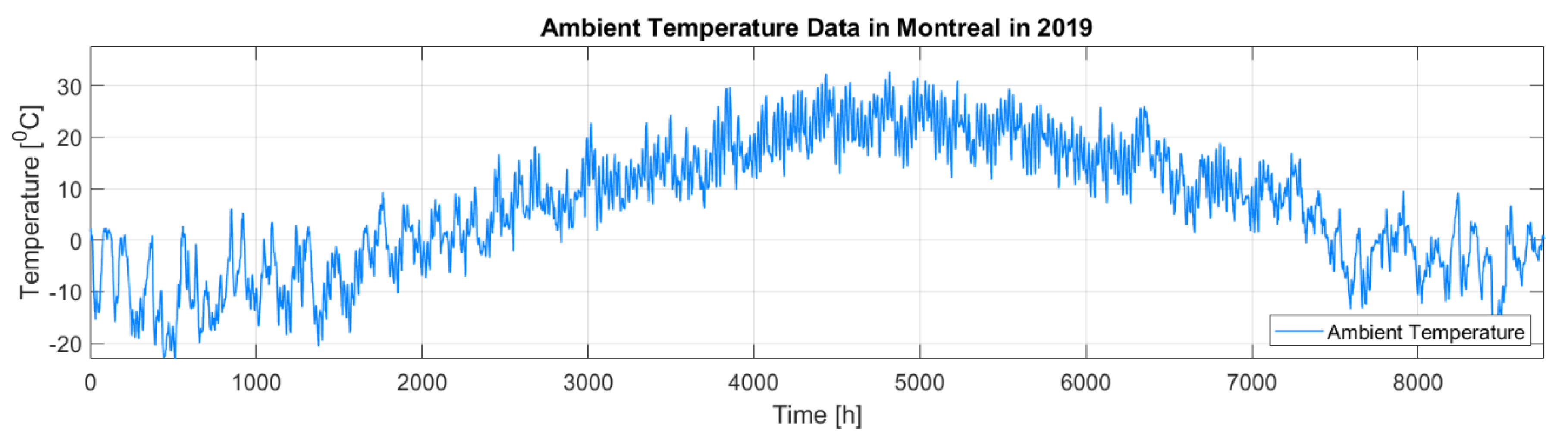
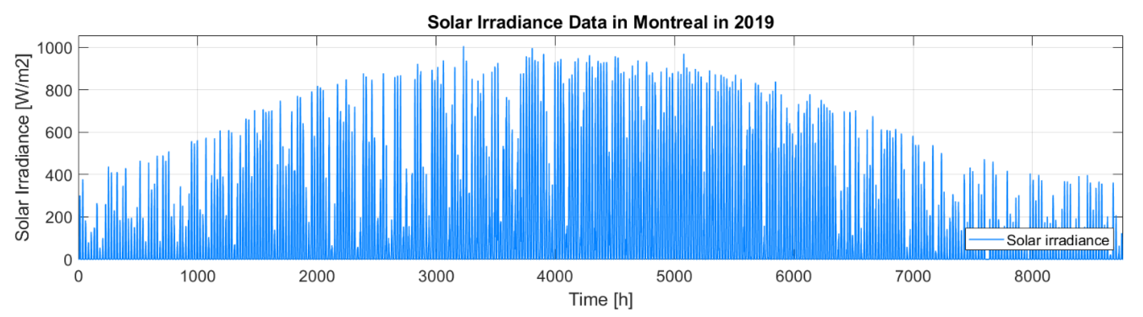
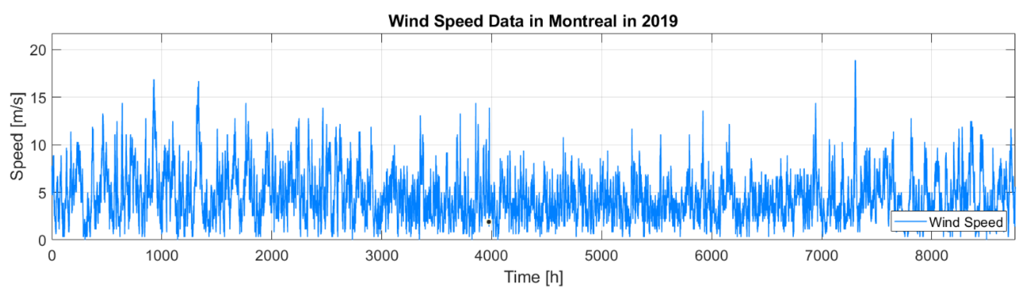
3.2. Real Data for the Montreal Case Study

To make the results more accurate, real weather and load data were necessary. Given this, we considered real weather data for the year 2019 as depicted in Figure 2 (ambient temperature), Figure 3 (solar irradiance), and Figure 4 (wind speed) [35]. In Figure 5, we estimate the hourly power demand profile of the EVs in the parking lot based on the EVs’ arrival and departure time to the supermarket. In most of the studies regarding the PV system design, only solar irradiance is considered and not the ambient temperature to simplify the calculation. However, this might not be very accurate because the ambient temperature significantly influences the output results, especially for regions like Canada. The reason is that the fluctuation of the ambient temperature can vary from −40 °C (in winter) to +40 °C (in summer), which affects the output power of the PV system. Hence, in this study, both ambient temperature and solar irradiance are considered for the PV system design.

3.3. Solar Panels’ Data

Table 1 shows a selected list of 11 solar panels from different manufacturers taken from the software “SAM 2018.11.11”, which will be used in our study. SAM is an abbreviation of System Model Advisor software adopted and developed by National Renewable Energy Laboratory (NREL) in Washington, D.C. USA. In fact, the software shows more than 24,590 different SP models. In this paper, only 11 solar panels were selected for simulation purposes. However, our proposed optimization algorithm can also work for the complete list of solar panels.

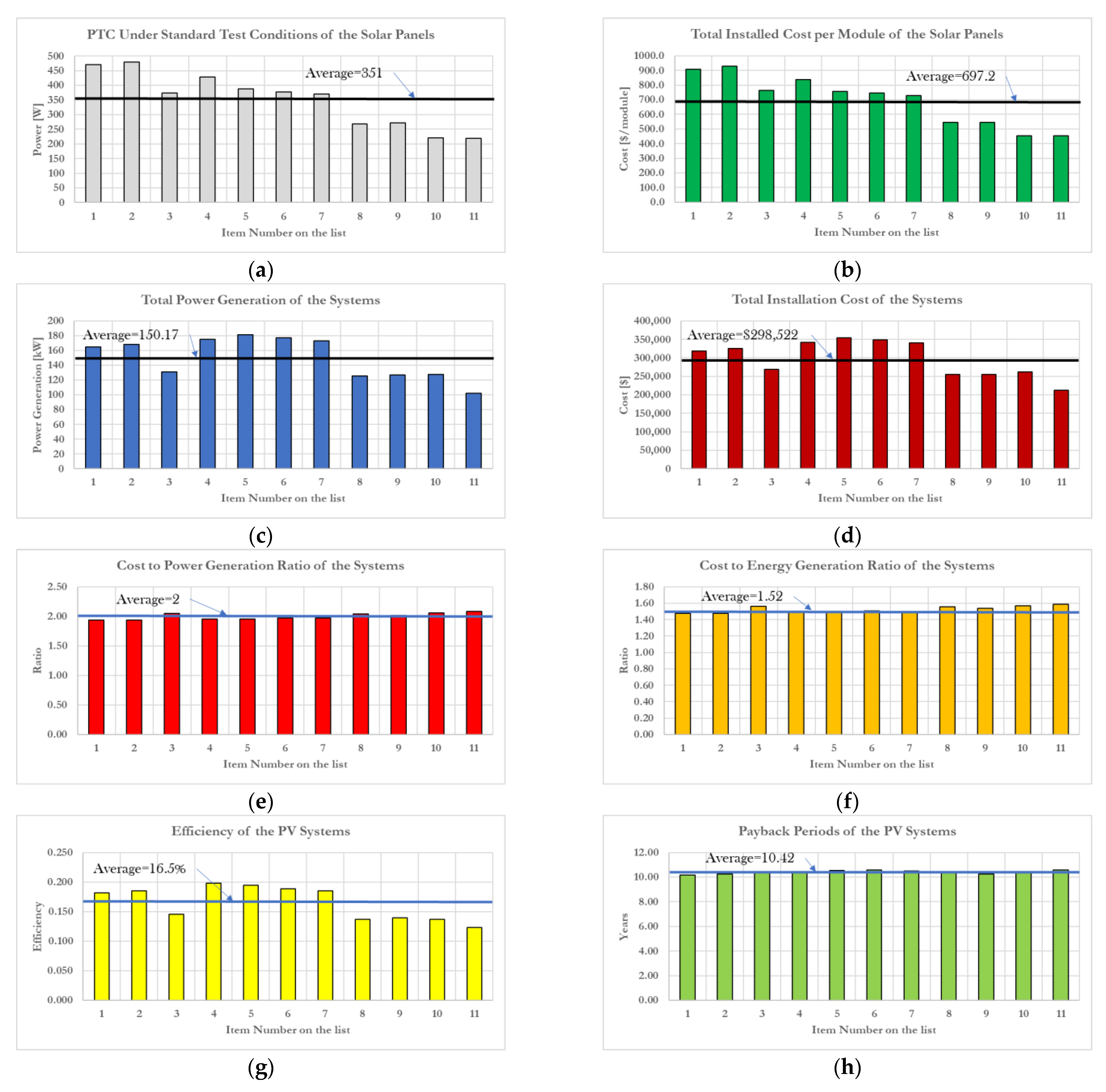
4. Results and Discussion

In this section, we present the results of the proposed RWR optimization algorithm and compare it to TOPSIS for validation purposes. First, we design the EVPL’s roof-mounted PV system in order to determine the available roof area that we can use in an optimal way, as in Section 4.1. In Section 4.2, we calculate the system’s performance using the proposed RWR optimization algorithm as in Algorithm 1, considering the data presented in Section 3 Table 1 and Figure 1, Figure 2, Figure 3, Figure 4 and Figure 5. Based on the obtained results from Section 4.2, we determine the decision matrix and weighting factors as in Section 4.3 and Section 4.4, respectively. Then, the proposed RWR optimization algorithm and TOPSIS are compared regarding their simulation speed and similarities in ranking and selecting the best alternatives, as in Section 4.5. Afterward, the impact of selecting different solar panels on the distribution network is studied in Section 4.6. Finally, the impact of the current electricity tariff on the future of EVPL in Montreal is discussed in Section 4.7, in which we propose some tariff modifications in order to encourage the deployment of the EVs and the construction of EVPLs in Montreal.

4.1. Design of the Electric Vehicle Parking Lot’s (EVPL) Roof-Mounted Photovoltaic (PV) System

In this section, we design the roof-mounted PV system since the initial EVPL does not have a roof. In the design, we consider many factors such as but not limited to the dimension of the parking lot, the elevation and azimuth angles, the positioning of the cars, the allowed height of the roofs, the spacing between roofs, etc. Based on the available data, Figure 6 shows our design of the EVPL’s roof. In total, the available roof area to install the PV system is equal to 1008 m2.

4.2. Calculation of the System Performance

After determining all the inputs of Algorithm 1 (lines: 1–6), the system’s performance is calculated in Algorithm 1 (lines: 7–20). Results are shown in Table 2, which are divided into two parts. Input data of the algorithm is presented in the first part, while the output data and corresponding equations for calculation are presented in the second part of Table 2. Figure 7 illustrates the output results of Table 2. There is a high correlation between Figure 7a,b, in which the installation cost per module is proportional to the output power of the SP. This is also demonstrated in Figure 7e,f, where the cost to power and cost to energy generation ratios of all SPs have almost constant values. We can predict an SP’s cost based on the output power (PTC) or the output generated energy. For example, suppose that a new SP becomes available in the market, and it generates 2000 W; the CPR is equal to 2. Hence the cost will be equal to 4000 $/module. On the other hand, it can be remarked that the SP with the maximum output power per module (e.g., item 1 and 2 in Figure 7c) might not produce the highest power generation for the complete system as in the case of items 4, 5 and 6 of Figure 7c. Moreover, a high cost per module does not mean that the total system’s cost will be increased, as presented in Figure 7d, in which items 1 and 2 have the highest cost per module, but not the highest for the complete PV system. In addition, Figure 7g demonstrates that SPs with the highest power output and the highest cost might not have the highest efficiencies. Figure 7h presents the PBP, which looks very similar to all SPs. However, these values may vary a lot when the selling electricity price supplied by the PV system changes. For a specific time, a selling electricity price of 15 ¢/kWh from the PV system to the EVs affects the results compared to a price of 10, 20, or 30 ¢/kWh, and the item with the lowest PBP might not be the ideal one for the EVPL. Figure 7i presents the ESSR, in which item 5 has the highest ratio, which is not expected since it does not have the highest output power nor the highest installation cost. It becomes satisfying to see that the ESSR and PSSR in Figure 7i,j are high enough to supply a large part of the EVPL’s energy demand. Therefore, it can be concluded that the future of the EVPL with a roof-mounted PV system is prominent, and it would be possible with the advancement of the PV technology to design a fully self-powered EVPL. Figure 7k shows the number of SPs to be installed on the roof, which depends on the SPs’ dimensions. The higher the output power is, the fewer SPs will be installed. Finally, Figure 7l shows the surface filling ratio (SFR) of the PV systems. The average ratio is about 90%, which is considered acceptable and validates our algorithm’s efficiency. Items 5, 6, and 7 have the highest SFRs, where item 11 has the lowest.

4.3. Decision Matrix

Table 2 and Figure 7 present interesting results for the decision-makers. However, it becomes confusing when contradictory results might not lead to the selection of the best PV system for the EVPL. Hence, it becomes essential to use advanced multi-criteria decision-making algorithms to select the best SP for a specific application. To do so, it is important to choose the most relevant criteria for the decision-maker for better decisions. Table 3 shows the decision matrix with the most relevant criteria used in our proposed RWR optimization algorithm for comparison and selecting the best SPs. After creating the decision matrix, the RWR optimization algorithm is compared to the well-established TOPSIS method for three different case scenarios in order to study their similarities in ranking and selecting the best alternatives and compare their simulation speed.

4.4. Determination of the Weighting Factors

The weighting factor for each criterion is determined in this paper for comparison purposes between the TOPSIS and RWR algorithms. Table 4 presents the weighting factor for each criterion for three different scenarios.

4.5. Comparing RWR and TOPSIS Methods under Different Test Conditions

In this subsection, the RWR and TOPSIS algorithms are compared for the three aforementioned scenarios in Table 4, and the results for ranking alternatives are presented in Table 5. The yellow color presents the best alternative, while the dark red color presents the worst one, as shown in Figure 8. The ranking of the alternatives for each criterion (criteria 1 to 9 in columns 4 to 12) is only considered in the RWR algorithm since TOPSIS does not allow the ranking of alternatives. TOPSIS classifies the final results, which are presented on the right side of Table 5. It is remarked that for scenario 1, the difference in ranking between RWR and TOPSIS is not very large since rank #1 in TOPSIS coincides with rank #3 in RWR. For the second scenario, both algorithms’ ranking is almost similar, and rank #1 in TOPSIS is the same as in RWR. Finally, scenario 3 presents the largest difference between TOPSIS and RWR, in which the rank #1 in TOPSIS is the last one in RWR. Therefore, both methods give different results for the aforementioned weighting factors. The question that arises is, how much are both methods similar? In the three different scenarios, we found that the difference in ranking between RWR and TOPSIS varies from very similar (Scenario 2) to not similar (Scenario 3).
To answer the previous question, we ran both algorithms 100 times for different weighting factors and compared the similarities under different conditions. Figure 9 presents the results of the 100 simulations. Figure 9a shows the difference in ranking between RWR and TOPSIS methods for the best alternative. A value equal to zero means that both methods choose the same best alternative and their similarity is very high (with a percentage of 40%). A value equal to 1 means that rank #1 in TOPSIS coincides with rank #2 in RWR (with a percentage of 20%). Results in Figure 9a show that more than 77% of the case scenarios, RWR and TOPSIS give similar results with a difference in ranking less than 2, which is considered good. This means that rank #1 in TOPSIS coincides with rank #3 or lower in RWR. Figure 9b shows the same results considering the percentage of the similarities instead of the difference in numbers. It also shows that 90–100% in ranking similarities between RWR and TOPSIS have a probability of 60%. The probability of getting a similarity between 80–90% is equal to 17%. In total, the probability of having 80–100% of ranking similarities is equal to 77%, which is remarkable. The next question is, why did we propose RWR instead of TOPSIS to select the best alternatives?
To answer the question, it is necessary to calculate the simulation time of both methods for different case scenarios as follows:
  • Case 1: the same dimension of the decision matrix is used while considering different weighting factors for each iteration, as in Table 6. In this case, RWR is faster than TOPSIS by 2.856 times;
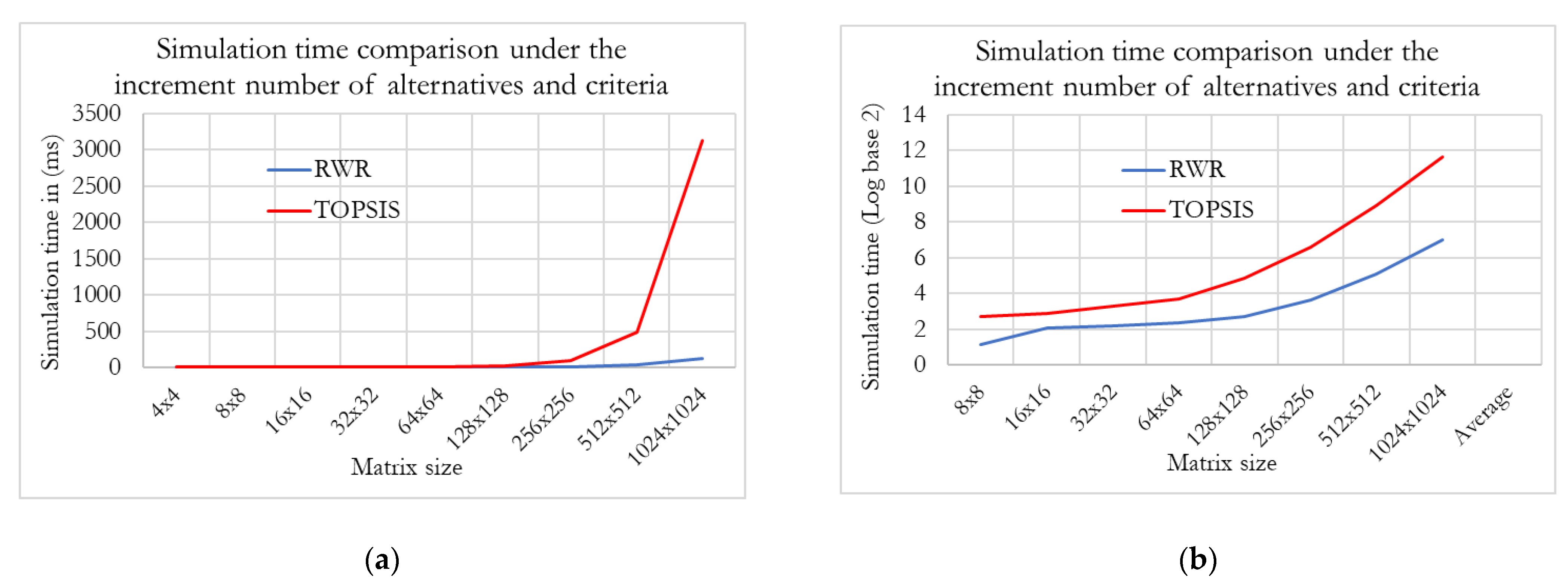
  • Case 2: the size of the decision matrix is doubled every iteration, as presented in Table 7 and Figure 10. The main goal is to know how much the matrix’s dimension affects the simulation time. In this case, it is remarked that RWR is much faster than TOPSIS, and the speed is exponentially increased with the increase of the decision matrix.
Table 8 presents a summary of the comparison between our proposed RWR and TOPSIS methods.

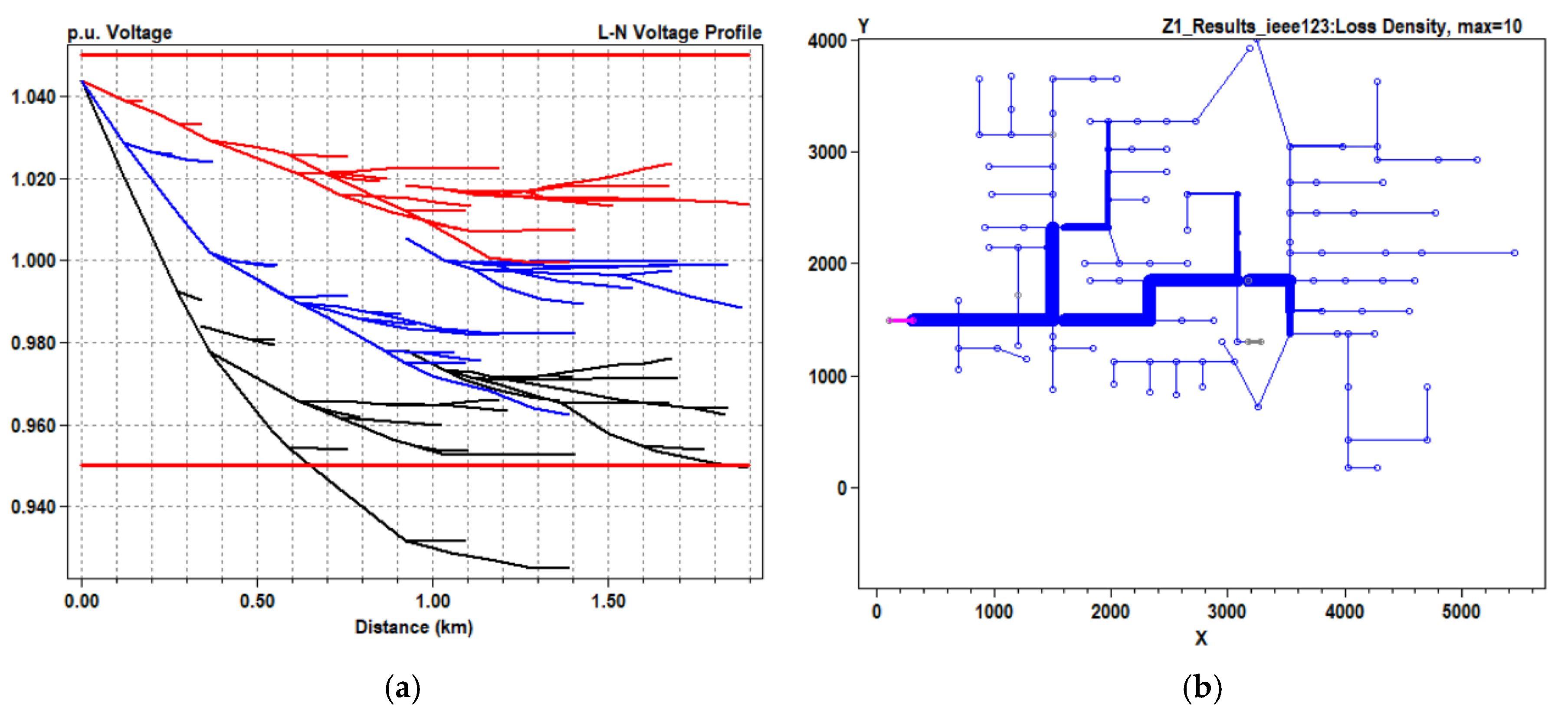
4.6. Does the Selection of Different Solar Panels Have an Impact on the Distribution System?

After studying the optimal selection of SPs, the question that can be asked is, “does the selection of different solar panels for a certain project impact the distribution network?” To answer this question, it is important to study the distribution system’s behavior when different solar panels are selected for a certain project. To do so, some assumptions are considered for this study for comparison purposes as follows:
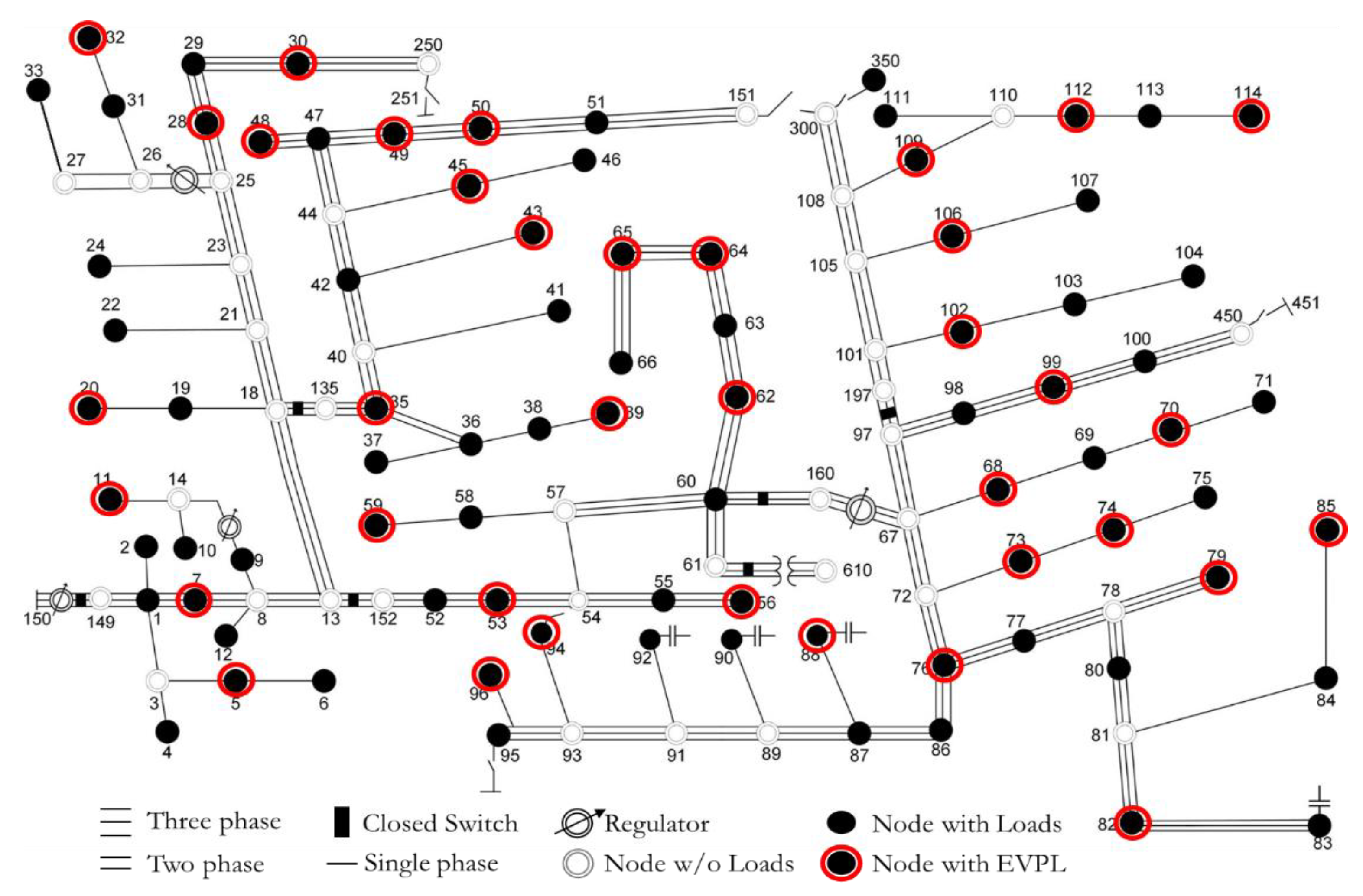
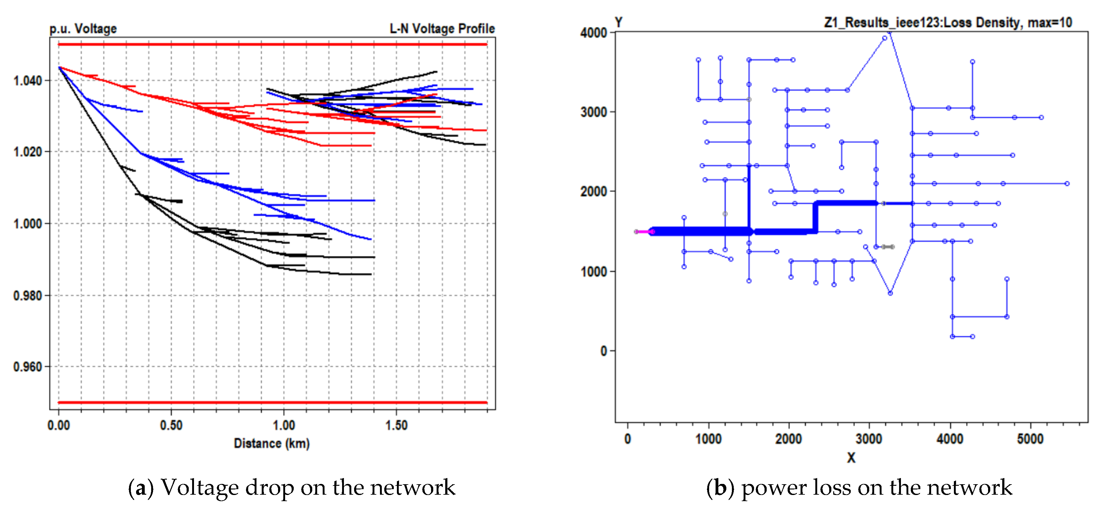
  • IEEE 123 nodes test feeder is considered as a distribution network (as in Figure 11);
  • We consider that 43% of the nodes have EVPLs (red dots in Figure 11);
  • OpenDSS is used to simulate the distribution network;
  • Since IEEE 123 is a standard network, we consider that the load of EVPL is added to the network.
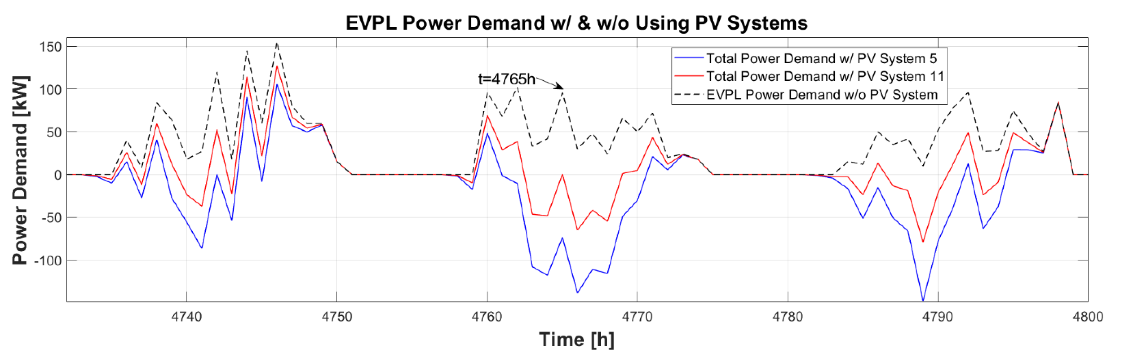
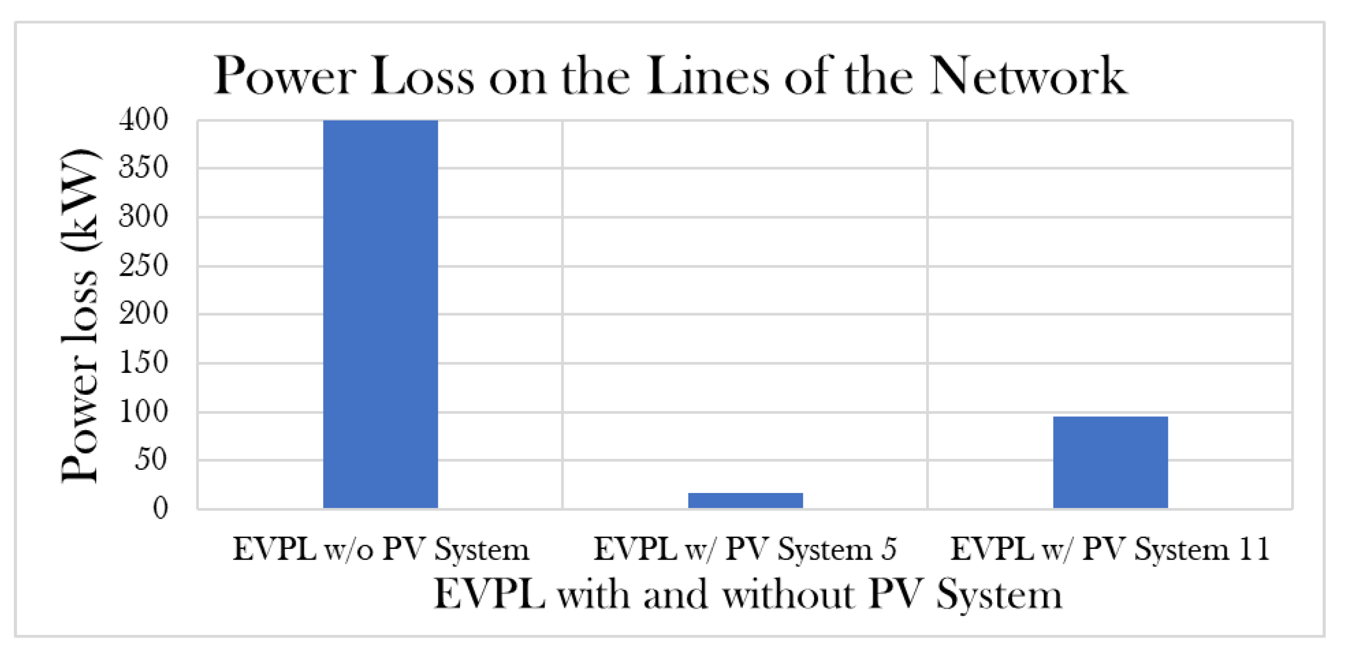
  • Solar panels items 5 (Canadian Solar Inc., model: CS1U-415MS) and 11 (Gintung Energy, model: ASEC-250G6S6B) are chosen for the comparison;
  • The same EVPL in the previous sections is studied with the same roof area to ensure a fair comparison;
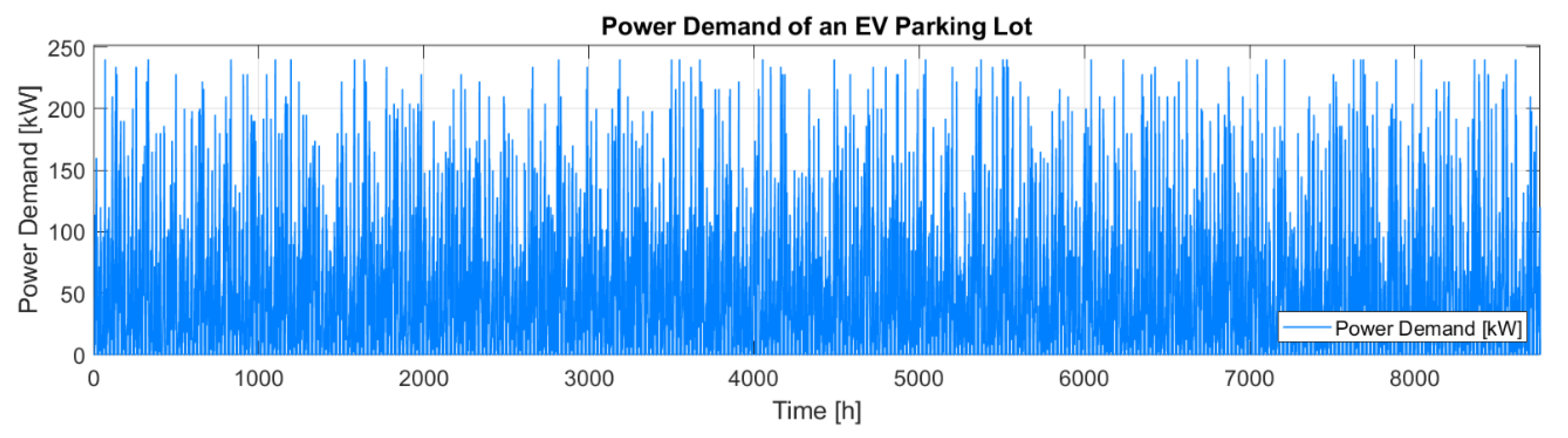
  • The comparison is made for t = 4765 h, which is on 2019-07-18 at 1 p.m. in the Montreal time zone as in Figure 12, where the local energy production is much higher than the energy demand;
  • Three scenarios are studied:
    Scenario 1: EVPL without using PV system (as in Figure 12, dashed black curve).
    Scenario 2: EVPL with PV system #5 (selecting SP #5) (as in Figure 12, blue curve).
    Scenario 3: EVPL with PV system #11 (selecting SP 1) (as in Figure 12, red curve).
    The main goal of studying these three different scenarios is to see how much the selection of different SPs impacts the distribution network, which is presented in Figure 13, Figure 14, Figure 15 and Figure 16.
Scenario 1: Figure 13 presents the impact of an EVPL without a PV system on the network at t = 4765 h (as in Figure 12, dashed black color). It can be remarked that some parts of the network have voltage drops below the recommended limit and the power losses are high. This is due to the fact that most of the EVPLs are consuming lots of electricity from the network, especially in peak periods when lots of EVs are charging at the same time.
Scenario 2: On the other hand, Figure 14 presents the impact of EVPLs with a PV system #5 ( i = 5 in Table 5) on the network. Results are better than the first scenario. However, we can see that there is a rise in voltage on some nodes, which exceeds the voltage limit of 1.05 per unit (p.u.). The reason is that there is an excess of energy production from the PV system #5 (refer to Figure 12 blue curve, at t = 4765 h), which exceeds the energy demand of the EVPL. Since 43% of the network’s nodes have EVPLs, the excess of energy production from all these EVPLs is injected into the grid and may cause a rise in the voltage in some periods. The voltage rise might happen just when there is lots of local energy production and less energy consumption. This problem could be solved by using optimization techniques to schedule the charging of the EVs in a way that avoids any problems on the network. Another option is to install a battery storage system in the EVPL, which can absorb the excess of energy generation and deliver it when needed; however, this option is costly. It can also be remarked that the power loss on the network is much less than the first case scenario as in Figure 14b and Figure 16, which will reduce the financial losses of the distribution system operator.
Scenario 3:Figure 15 presents the impact of an EVPL with a PV system #11 ( i = 11 in Table 5) on the network. Results are better than both previous scenarios because the voltage drop is maintained within limits (0.9 p.u., and 1.05 p.u.). However, this is just a particular case (for t = 4765 h in Figure 12 for red curve). This might not be true for other cases. In general, the energy production from PV system #11 is less than PV system #5 and may not improve the voltage profile in many cases. Moreover, the power loss on the network is less than in scenario 1 but much higher than scenario 2, as it is shown in Figure 15b and Figure 16.
It can be concluded that the selection of different solar panels, even for the same project with the same installed surface, can have an impact on the network. Figure 13, Figure 14, Figure 15 and Figure 16 show a particular case where the local energy generation is higher than the consumption, which does not often happen since the PV system’s energy production can be less than the demand for different users. However, the main goal of studying this particular case is to show that the selection of different solar panels can affect the voltage and power losses on the network, especially when the penetration level of PV systems on the network increases and could reach a level of destabilizing the grid. This problem can be solved using some optimization algorithms on different levels, as discussed in our previous work [6,36,37,38,39]. Hence, it is clear that selecting the best SP for a specific application should be made using advanced tools such as MCDM algorithms. Moreover, the selection should be accompanied by a complete study of the techno-economic impact on both client and the system operator. However, the question arises: does the power utility Hydro-Quebec incite users to install renewable energy technologies with the current electricity tariffs? The next subsection answers this question.

4.7. The Impact of the Electricity Tariff on the Future of Electric Vehicle Parking Lot

In the case where all rate M fees are applied to the parking lot, the EVPL owner has to pay almost 41,990.4$/year as a subscription fee for using 240 kWp, which is considered very high and not profitable for the EVPL owner. Hence, he is obliged to raise the electricity cost to more than 36¢/kWh for a PBP of almost 10 years, without considering the civil infrastructure’s investment cost or the employees’ salaries. Therefore, the investment in an EVPL in Montreal is not a good idea, and the transition from internal combustion engine cars to EVs becomes difficult since no one is interested in investing in a project with such a high PBP and low income. To solve the problem and to encourage the deployment of EVs in the market, we propose some solutions in which the government of Quebec can take into account to promote the construction of EVPLs as follows:
  • Reduce the subscription fees for an EVPL by considering only the energy consumption. It is possible a small monthly subscription fee can be applied;
  • Encourage the EVPLs to integrate renewable energy systems such as PV and wind turbines to increase their ESSR;
  • Subsidies and funding can be applied to reduce the investment cost of renewable energy sources such as PV systems, wind turbines, etc. Hence, the EVPL will be able to produce more local energy and will reduce the demand from the electrical network;
  • Optimization should be used to manage the charging of EVs and minimize the peak demand. Therefore, the impact on the electrical network is reduced;
  • Bidirectional chargers could also reduce the impact on the network and may increase the revenue of the EVPL owner by participating in ancillary services.

5. Conclusions and Future Work

This paper presented an original rank-weigh-rank (RWR) optimization algorithm for ranking and selecting the best solar panels for the case of electric vehicle parking lots (EVPLs) with roof-mounted PV systems. The main goal was to maximize the local energy production and the energy self-sufficiency ratio, while reducing the payback period of the PV system. In addition, the proposed RWR optimally distributes the solar panels on the roofs of the EVPL in a way that maximizes the surface filling ratio. A case study in Montreal was considered in which we designed a roof-mounted PV system for an EVPL. To validate our proposed optimization algorithm, we compared RWR with the well-established TOPSIS method, and we studied the impact of selecting and not selecting the best solar panels on the distribution network. Results show that our proposed RWR is much faster than TOPSIS, especially when the size of the decision matrix becomes larger. Also, there are similarities in selecting the same best SP in more than 40% of cases, while more than 77% of the cases give a similarity with more than 80% for selecting the best SPs. To make the study more realistic, the techno-economic impact of selecting different SPs on the decision-maker and the distribution system operator is studied, in which it shows that the selection of SP is critical in reducing the techno-economic losses, which were not done before, as per the best knowledge of the authors. For instance, selecting the PV system #5 (Canadian Solar Inc., model: CS1U-415MS) instead of #11 (Gintung Energy, model: ASEC-250G6S6B) has increased the local energy generation of the EVPL. Hence, it has increased the income of the EVPL owner and reduced the energy demand from the distribution network, which will reduce the voltage drop and power loss on the lines and the transformer. Hence, both the decision-maker and the system operator are satisfied. However, there are lots of barriers that should be considered in our future work:
  • the electricity tariff in Quebec does not encourage the decision-makers to build an EVPL in Montreal since the electricity tariff is very high, and the construction cost is also very high, which should be reconsidered;
  • the PV system is insufficient to supply the EVPL’s demand, especially in Quebec, since the solar radiation is low most of the time, even in summer. Hence, other renewable energy systems should be studied, such as the integration of vertical axis wind turbines;
  • the integration of renewable energy systems and EVs should always be accompanied with advanced tools to manage and schedule the energy generation and consumption to avoid problems on the network, as discussed previously;
  • since RWR and TOPSIS do not always give the same results, it becomes a little bit confusing to know which method is better than the other. From this place, it is necessary to study and compare many MCDM methods in order to see which ones are the most probable to use for the case of renewable energy-based EVPLs.

Author Contributions

Writing—original draft preparation, C.Z.E.-B.; writing—review and editing, M.Z., U.E. and N.S.; supervision, U.E.; funding acquisition, U.E. All authors have read and agreed to the published version of the manuscript.

Funding

This work was supported in part by the Canada Excellence Research Chairs Program and in part by the Tri-Agency Institutional Program Secretariat.

Institutional Review Board Statement

Not applicable.

Conflicts of Interest

The authors declare no conflict of interest.

Appendix A. Mathematical Modeling and Constraints of the Proposed Algorithm

The mathematical equations that are mentioned in the proposed algorithm are presented in this appendix for further reading.

Appendix A.1. Efficiency of the Solar Panel

Equation (A1) represents the efficiency ( η i P V ) of the SP “ i ” [33]. A higher maximum power generation of the system ( P M P P T , i P V ), increases its efficiency under standard test conditions (STC) for the same area of the panel A i P V in [m2]. Hence, a solar panel with higher efficiency generates more energy with the same installed surface. G S T C is the solar irradiance under standard test conditions ( G S T C = 1000 W/m2 and ambient temperature = 25 °C).
η i P V = P M P P T , i P V G S T C A i P V  

Appendix A.2. Total Number of the Installed Solar Panels

Let us suppose a case in which we want to install a PV system on a rectangular rooftop, as presented in Figure A1. Figure A2 shows the dimension of the i -th SP in which it has short and long sides, with a tilt angle ϕ . Consider that the short side ( X i P V ) is on the X-axis, and the long side ( Y i n c , i P V or L i P V ) is on the Y-axis. If all SPs do not have the same dimensions, and same output power rate, it becomes a difficult task to optimally size and distribute them on the rooftop, which is considered the main objective to be solved in this subsection.
Figure A1. Example of the distribution of solar panels on the rooftop.
Energies 14 04515 g0a1
Figure A2. Dimension of a solar panel.
Energies 14 04515 g0a2
Equation (A2) shows the maximum number of solar panels ( N R , i P V ) in a row on the X-axis. Where, X r o o f is the width of the rooftop; X j S is the space on the X-axis between two solar panels; X N R P V S is the space between the right boundary and the last solar panel; X i P V is the short side length of the solar panel; X 0 S is the space between the left boundary and the first solar panel; [ x ] 10 n B is the general round function suggested in this paper and expressed in Equation (A3). For example, [ 235.7235 ] 10 2 C = [ 235.7235 100 ] · 100 = [ 2.357235 ] · 100 = 3 · 100 = 300 ; [ 235.7235 ] 10 2 C = [ 235.7235 0.01 ] · 0.01 = [ 23572.35 ] · 0.01 = 23573 · 0.01 = 235.73 .
N R , i P V = { [ X f r o o f ( X 0 S + X N R P V S ) + X 1 S X i P V + X 1 S ] 10 n F     i f   X 0 S ,   X N R P V S ,   N j = 1 ( N R P V 1 ) P V   a r e   d e f i n e d [ X f r o o f j = 0 N R P V X j S X i P V ] 10 n F     e l s e
[ x ] 10 n B = { [ x 10 n ] · 10 n   i f   B = F ,   i t   i s   a   f l o o r   f u n c t i o n   [ x 10 n ] · 10 n   i f   B = C ,   i t   i s   a   c e i l i n g   f u n c t i o n ,   w h e r e   n
Equation (A4) presents the maximum number of solar panels on the Y-axis in a column ( N C , i P V ). Where, Y r o o f is the rooftop length on the Y-axis; Y j S is the spacing between two consecutive solar panels on the Y-axis; Y i P V presents the projection on the horizontal plan of the i -th solar panel, where Y i P V = Y i n c , i P V cos ( φ i ) ; Y 0 S shows the spacing between the south boundary and the first solar panel on the Y-axis; Y N C P V S is the spacing between the north boundary and the last solar panel on the Y-axis; all distance units are in [m]; φ i is the PV module’s inclination with respect to the horizon in [o].
N C , i P V = { [ Y r o o f ( Y 0 S + Y N C P V S ) + Y 1 S L i P V cos ( φ i ) + Y 1 S ] 10 n F     i f   Y 0 S ,   Y N C P V S ,   N j = 1 ( N C P V 1 ) P V   a r e   d e f i n e d [ Y r o o f j = 0 N C P V Y j S Y i P V ] 10 n F     e l s e
Equation (A5) presents the total number of SPs on F rectangular rooftops (with different dimensions); where, N C , i , f P V and N R , i , f P V are the maximum numbers of solar panels of type i arranged in a column and in a row on the rooftop f , respectively. E.g., for the rooftop f = 1 , N C , i , 1 P V = 6 , and N R , i , 1 P V = 7 , for rooftop f = 2 , N C , i , 2 P V = 8 , and N R , i , 2 P V = 5 , then N T o t a l , i P V = ( 6 · 7 + 8 · 5 ) = 82   SPs.
N T o t a l , i P V = f = 1 F N C , i , f P V N R , i , f P V

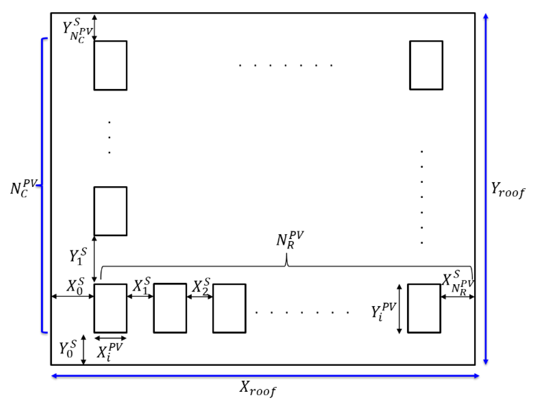
Appendix A.3. Installed Capacity of the Solar System

Equation (A6) presents the total installed capacity of the PV system ( P S T C , i P V   S y s ) under STC for the i -th alternative. Where, P M P P T , i P V is the maximum power generation of a solar panel “ i ” under STC and N T o t a l , i P V is the total number of solar panels on the rooftops for the alternative “ i ”.
P S T C , i P V   S y s = P M P P T , i P V · N T o t a l , i P V   ;     ( k W )

Appendix A.4. The Total Installation Cost of the PV System

Equation (A7) shows the total installation cost of the PV system of the i -th alternative ( C o s t i P V   S y s ), which is equal to the total investment cost per solar panel, including direct and indirect cost ( C o s t i P V ), multiplied by the total number of solar panels on all roofs ( N T o t a l , i P V ).
C o s t i P V   S y s = C o s t i P V · N T o t a l , i P V ;     ( $ )

Appendix A.5. Cost to Power Generation Ratio of the PV System under Standard Test Conditions (STC)

Equation (A8) presents the cost to power generation ratio of the i -th PV system ( C P R i P V   S y s ) in [$/kW], in which it shows the installed system cost per kW of generation under STC. An expensive system has a high ratio, while a cheap system has a low ratio.
C P R i P V   S y s = C o s t i P V   S y s P S T C , i P V   S y s ,     ( $ k W )

Appendix A.6. Cost to Energy Generation Ratio of the PV System under Real Weather Conditions

Equation (A9) presents the cost to energy generation ratio of the i -th PV system ( C E R i P V   S y s ), in which it shows the installed system cost per kWh of generation under real weather conditions for a period T where Δ t is the time step in (h). An expensive system has a high ratio, while a cheap system has a low ratio. Equation (A10) shows that the power of the PV system can supply the EVs and the grid when needed.
C E R i P V   S y s = C o s t i P V   S y s t T ( P i , t P V   S y s Δ t ) ,     ( $ k W )
where,
P i , t P V   S y s = P i , t P V 2 E V + P i , t P V 2 G

Appendix A.7. Payback Period

The payback period (PBP) presents the time it takes to attain a break-even point, in which the generated income or cash is equal to the investment cost for a certain investment [40]. The shorter the PBP is, the better the investment is considered. In general, investors are interested in minimizing as much as possible the PBP to return their investment cost as soon as possible and generate much more income. PBP is equal to the investment cost divided by the annual cash flows, as presented in Equation (A11). For example, a client invested 24,000$ to install solar panels on his roof. The generated electricity from the PV system allowed him to save 200 $/month. In this case, the PBP is equal to 10 years (24,000$/(200$ × 12)). In other words, it will take about 10 years to reach a break-even point and return his invested money.
P a y b a c k   P e r i o d = C o s t   o f   I n v e s t m e n t A n n u a l   C a c h   F l o w s  
In this paper, an EVPL with a roof-mounted PV system is studied. Hence, Equation (A12) is proposed instead of Equation (A11) to fit the studied case; where,   C o s t i P V   S y s is the total investment cost of the i -th alternative PV system. ε t P V 2 E V and ε t P V 2 G are the price of the sold electricity to the EVs and to the grid, respectively. P i , t P V 2 E V and P i , t P V 2 G are the power generation from the PV system that supplies the EVs and the grid, respectively. t i and t f represent the starting and ending time of the study. P t E V P L is the power consumption of the EVPL at instant “ t ” in [kW]. In this paper, the study is done for a complete year, therefore t f t i = 8760   h . P i , t P V   S y s ; > P t E V P L ; ( 1 ) / ( 0 ) _ is an infomath function, which means, if P i , t P V   S y s > P t E V P L , replace the infomath equation by 1, else, replace it by zero. The advantage of using infomath functions is to unify many equations into only one [41]. P n , t G 2 E V and P n , t E V 2 G are the power from grid to EV and from EV to grid respectively, as presented in Equation (A13). α n E V and β n E V are decision variables in which the EVs can either charge or discharge as in Equation (A14). The power demand from the EVPL ( P t E V P L ) considers both V2G and G2V strategies which might affect the optimal selection of the solar panels in a way to supply the demand with the shortest payback period.
P B P i P V   S y s = C o s t i P V   S y s t = t i t f ( ε t P V 2 E V P i , t P V 2 E V + ε t P V 2 G P i , t P V 2 G · P i , t P V   S y s ; > P t E V P L ; ( 1 ) / ( 0 ) _ ) Δ t  
where,
P t E V P L = n = 1 N E V ( α n E V P n , t G 2 E V β n E V P n , t E V 2 G ) + P i , t P V 2 E V
α n E V + β n E V 1 ,   α n E V , β n E V
The energy demand of the EVPL during the period T = [ t i ,   t f ] is expressed in Equation (A15). This energy should be supplied from both the PV system ( t = t i t f ( P i , t P V 2 E V ) Δ t ) and from the grid ( n = 1 N E V t = t i t f ( α n E V P n , t G 2 E V Δ t ) ). In case some EVs participate in the ancillary services and inject active power to the grid, the injected energy ( n = 1 N E V t = t i t f ( β n E V P n , t E V 2 G Δ t ) Δ t ) should also be added in order to reach the final state of charge as desired by the EV owners.
t = t i t f P t E V P L Δ t = t = t i t f ( P i , t P V 2 E V Δ t ) + n = 1 N E V t = t i t f ( α n E V P n , t G 2 E V Δ t ) + n = 1 N E V t = t i t f ( β n E V P n , t E V 2 G Δ t )

Appendix A.8. Output Power of the PV System

Equation (A16) presents the output power of the i -th alternative PV system at instant “ t ” ( P i , t P V   S y s ). Where the output power from the solar system can supply the EVs ( P i , t P V 2 E V ) and/or inject power to the grid ( P i , t P V 2 G ). Equation (A17) describes the output energy of the PV system “ i ”during a period T (e.g., 1 year).
P i , t P V   S y s = G t 1000 η i P V A i P V N T o t a l , i P V ,     ( kW )  
E i P V   S y s = t T P i , t P V   S y s Δ t ,     ( kWh )  

Appendix A.9. Energy Self-Sufficiency Ratio

In this paper, we define the energy self-sufficiency ratio (ESSR) as the ratio of the local energy production for a unit (such as parking lot, building, city, district, etc.) from renewable energy technologies divided by the energy demand of the unit over a period T (e.g., minutes, hours, days, months, years), as described in Equation (A17). If ESSR = 1, the produced and consumed energy are equal. Hence, the unit is considered as energy self-sufficient. If ESSR < 1, the produced energy is less than the energy demand of the unit. Therefore, another external energy source has to be used to meet the gap between energy production and demand. If ESSR >1, the unit is capable of producing more energy than its needs. Consequently, the extra energy production can be sold to the grid or any other external consumer.
E S S R T , i = E n e r g y   p r o d u c e d T , i E n e r g y   c o n s u m e d T = t = t i t f ( P i , t P V   S y s Δ t ) t = t i t f ( P t E V P L Δ t )

Appendix A.10. Power Self-Sufficiency Ratio

In this paper, the power self-sufficiency ratio (PSSR) is proposed to be the percentage of time in which a unit (e.g., EVPL) can generate its own power that is greater or equal to its instantaneous power needs without being supplied from the electrical network. For example, if PSSR = 40%, it means that the unit is able to supply its demand 40% of the time. This factor is essential since it gives an indication to the decision-maker about whether he needs to install a battery storage system or any other source of energy generation, and it tells the decision-maker how much-generated electricity can be sold to the grid.
  • If PSSR = 0%, it means that the PV system is not able to meet the demand of the unit, whatever is t. Therefore, it might not be necessary to install batteries to store energy since there is no excess in production.
  • If PSSR = X% where X % [ 0 , 100 % ] , it means that the PV system is able to meet the demand for X% of the time. In this case, if the excess in power production is high in some periods, the decision-maker can install a battery storage system (BSS) in order to store the excess of energy and to use it later once the unit needs it,
  • If PSSR = 100%, it means that the PV system is always producing more energy than needed at any time t. Hence, the decision-maker can sell the energy to the grid without even installing a BSS.
To calculate the PSSR, the following algorithm is proposed. The first step is to define the parameters t i , Δ t , T and N M e t   P o w e r . Then calculate N and t f . After that, count the number of times when the power production is higher than the power demand ( P i ,   t = t i + N · Δ t P V   S y s P t = t i + N · Δ t E V P L ). Finally, calculate PSSR, which is equal to the reached power divided by the total number of time steps; or, we can use the infomath function [41], which summarizes the whole algorithm in a simple mathematical equation as we have proposed in Equation (A18). The PSSR will not be used in the decision matrix; however, it is a good tool to compare different renewable energy technologies.
Algorithm A1. Proposed Algorithm
1 Define:
2     t i    %Starting time of the study e.g., t i = 8   am
3     Δ t   %Time interval, e.g., Δ t = 1   h
4     T    %Period of the study, e.g., 24 h
5     N Met   Power = 0  %Initialize the number of met demand by the power production
6 Calculate:
7     N = T Δ t ; %Number of step intervals
8     t f = t i + N · Δ t ; % ending time of the study, e.g., t f = 11   pm
9 for n = 0 N
10  if P i , t = t i + N · Δ t PV   Sys P t = t i + N · Δ t EVPL
11    N Met   Power = N Met   Power + 1 % Count the number of times when the generated power meets the power demand
12  end if
13 end for
14  PSSR = N Met   Power N 100 % %Power Self-Sufficiency Ratio
End of Algorithm
P S S R i = t = t i t i + T ( P i , t P V   S y s ; < P t E V P L ; ( 1 ) / ( 0 ) _ ) T Δ t

Appendix A.11. Excess and Lack of Energy Production Ratios

In this paper, we propose two mathematical equations to calculate the performance of a PV system. The first one is called the excess of energy production ratio (EEPR), which is described in Equation (A19), in which it sums up only the energy production higher than the energy consumption at instant t for the period T . The second one is called the lack of energy production ratio (LEPR), which is described in Equation (A20), in which it sums up only the lack of energy supply when the energy production is lower than the consumed one. EEPR and LEPR will not be used in this paper’s decision matrix; however, they are useful tools to compare different renewable energy technologies.
E E P R i   = t = t i t i + T ( P i , t P V   S y s ; > P t E V P L ; ( P i , t P V   S y s P t E V P L ) / ( 0 ) _ ) t = t i t i + T P t E V P L
L E P R i = t = t i t i + T ( P i , t P V   S y s ; P t E V P L ; ( P t E V P L P i , t P V   S y s ) / ( 0 ) _ ) t = t i t i + T P t E V P L

Appendix A.12. Surface Filling Ratio

After calculating the required number of solar panels and positioning them on the roof, it is important to know how much surface is used to install the solar panels. Therefore, we introduce the surface filling ratio (SFR) as an efficient tool to compare the used surface by the solar panels with respect to the roofs’ total surface; where, N T o t a l P V is the total number of solar panels, in which the area of each panel is A i P V ; A T o t a l R o o f is the total area of all roofs (from roof r = 1 to roof r = R ) in which we intend to install solar panels. Please note that sometimes we have many roofs with different dimensions. Therefore, we calculate the number of SPs for each roof; then, we sum up all of them. SFR will not be used in this paper’s decision matrix; however, it is used as a good tool for a comparison of the results.
S F R i P V   S y s = N T o t a l , i P V A i P V A T o t a l R o o f 100 %  
where,
N T o t a l , i P V = f = 1 F N C , i , f P V N R , i , f P V
A T o t a l R o o f = f = 1 F A f R o o f  

References

  1. Tan, K.M.; Ramachandaramurthy, V.K.; Yong, J.Y. Integration of electric vehicles in smart grid: A review on vehicle to grid technologies and optimization techniques. Renew. Sustain. Energy Rev. 2016, 53, 720–732. [Google Scholar] [CrossRef]
  2. Harris, S.; Weinzettel, J.; Bigano, A.; Källmén, A. Low carbon cities in 2050? GHG emissions of European cities using production-based and consumption-based emission accounting methods. J. Clean. Prod. 2020, 248, 119206. [Google Scholar] [CrossRef]
  3. Ilieva-Obretenova, M. Information Model for City Monitoring by Smart Lighting. J. Min. Geol. Sci. 2018, 61, 55–59. [Google Scholar]
  4. Rajakaruna, S.; Shahnia, F.; Ghosh, A. Plug in Electric Vehicles in Smart Grids; Springer: Berlin/Heidelberg, Germany, 2016. [Google Scholar]
  5. Mohsenzadeh, A.; Pazouki, S.; Haghifam, M.R.; Chengzong, P. Optimal planning of parking lots and demand response programs in distribution network considering power loss and voltage profile. In Proceedings of the Innovative Smart Grid Technologies Conference (ISGT), 2015 IEEE Power & Energy Society, Washington, DC, USA, 18–20 February 2015; pp. 1–5. [Google Scholar]
  6. El-Bayeh, C.Z.; Mougharbel, I.; Asber, D.; Saad, M.; Chandra, A.; Lefebvre, S. Novel approach for optimizing the transformer’s critical power limit. IEEE Access 2018, 6, 55870–55882. [Google Scholar] [CrossRef]
  7. The World’s Biggest Solar Photovoltaic Cell Manufacturers. Available online: https://www.power-technology.com/features/featurethe-worlds-biggest-solar-photovoltaic-cell-manufacturers-4863800/ (accessed on 4 May 2021).
  8. Huang, Q.; Jia, Q.-S.; Guan, X. A Review of EV Load Scheduling with Wind Power Integration. IFAC-Pap. 2015, 48, 223–228. [Google Scholar] [CrossRef]
  9. Li, D.; Heimeriks, G.; Alkemade, F. The emergence of renewable energy technologies at country level: Relatedness, international knowledge spillovers and domestic energy markets. Ind. Innov. 2020, 27, 1–23. [Google Scholar] [CrossRef] [Green Version]
  10. Adefarati, T.; Obikoya, G. Assessment of Renewable Energy Technologies in a Standalone Microgrid System. Int. J. Eng. Res. Afr. 2020, 46, 146–167. [Google Scholar] [CrossRef]
  11. Moustakas, K.; Loizidou, M.; Rehan, M.; Nizami, A. A review of recent developments in renewable and sustainable energy systems: Key challenges and future perspective. Renew. Sustain. Energy Rev. 2020, 119, 109418. [Google Scholar] [CrossRef]
  12. Boxwell, M. Solar Electricity Handbook 2019 Edition: A Simple Practical Guide to Solar Energy: Designing and Installing Solar PV Systems; Greenstream Publishing: Coventry, UK, 2019. [Google Scholar]
  13. Fazelpour, F.; Vafaeipour, M.; Rahbari, O.; Rosen, M.A. Intelligent optimization to integrate a plug-in hybrid electric vehicle smart parking lot with renewable energy resources and enhance grid characteristics. Energy Convers. Manag. 2014, 77, 250–261. [Google Scholar] [CrossRef]
  14. Zhang, Y.; Cai, L. Dynamic Charging Scheduling for EV Parking Lots With Photovoltaic Power System. IEEE Access 2018, 6, 56995–57005. [Google Scholar] [CrossRef]
  15. Turan, M.T.; Ates, Y.; Erdinc, O.; Gokalp, E.; Catalão, J.P.S. Effect of electric vehicle parking lots equipped with roof mounted photovoltaic panels on the distribution network. Int. J. Electr. Power Energy Syst. 2019, 109, 283–289. [Google Scholar] [CrossRef]
  16. Ghazvini, A.M.; Olamaei, J. Optimal sizing of autonomous hybrid PV system with considerations for V2G parking lot as controllable load based on a heuristic optimization algorithm. Sol. Energy 2019, 184, 30–39. [Google Scholar] [CrossRef]
  17. Velasquez, M.; Hester, P.T. An analysis of multi-criteria decision making methods. Int. J. Oper. Res. 2013, 10, 56–66. [Google Scholar]
  18. Kumar, A.; Sah, B.; Singh, A.R.; Deng, Y.; He, X.; Kumar, P.; Bansal, R. A review of multi criteria decision making (MCDM) towards sustainable renewable energy development. Renew. Sustain. Energy Rev. 2017, 69, 596–609. [Google Scholar] [CrossRef]
  19. Ananda, J.; Herath, G. A critical review of multi-criteria decision making methods with special reference to forest management and planning. Ecol. Econ. 2009, 68, 2535–2548. [Google Scholar] [CrossRef]
  20. Agarwal, P.; Sahai, M.; Mishra, V.; Bag, M.; Singh, V. A review of multi-criteria decision making techniques for supplier evaluation and selection. Int. J. Ind. Eng. Comput. 2011, 2, 801–810. [Google Scholar] [CrossRef]
  21. Wang, J.-J.; Jing, Y.-Y.; Zhang, C.-F.; Zhao, J.-H. Review on multi-criteria decision analysis aid in sustainable energy decision-making. Renew. Sustain. Energy Rev. 2009, 13, 2263–2278. [Google Scholar] [CrossRef]
  22. Kabir, G.; Sadiq, R.; Tesfamariam, S. A review of multi-criteria decision-making methods for infrastructure management. Struct. Infrastruct. Eng. 2014, 10, 1176–1210. [Google Scholar] [CrossRef]
  23. Scott, J.A.; Ho, W.; Dey, P.K. A review of multi-criteria decision-making methods for bioenergy systems. Energy 2012, 42, 146–156. [Google Scholar] [CrossRef] [Green Version]
  24. Penadés-Plà, V.; García-Segura, T.; Martí, J.V.; Yepes, V. A review of multi-criteria decision-making methods applied to the sustainable bridge design. Sustainability 2016, 8, 1295. [Google Scholar] [CrossRef] [Green Version]
  25. Mardani, A.; Zavadskas, E.K.; Khalifah, Z.; Zakuan, N.; Jusoh, A.; Nor, K.M.; Khoshnoudi, M. A review of multi-criteria decision-making applications to solve energy management problems: Two decades from 1995 to 2015. Renew. Sustain. Energy Rev. 2017, 71, 216–256. [Google Scholar] [CrossRef]
  26. Sabaei, D.; Erkoyuncu, J.; Roy, R. A review of multi-criteria decision making methods for enhanced maintenance delivery. Procedia CIRP 2015, 37, 30–35. [Google Scholar] [CrossRef] [Green Version]
  27. Shao, M.; Han, Z.; Sun, J.; Xiao, C.; Zhang, S.; Zhao, Y. A review of multi-criteria decision making applications for renewable energy site selection. Renew. Energy 2020, 157, 377–403. [Google Scholar] [CrossRef]
  28. Balo, F.; Şağbanşua, L. The Selection of the Best Solar Panel for the Photovoltaic System Design by Using AHP. Energy Procedia 2016, 100, 50–53. [Google Scholar] [CrossRef] [Green Version]
  29. Wang, T.-C.; Tsai, S.-Y. Solar panel supplier selection for the photovoltaic system design by using fuzzy multi-criteria decision making (MCDM) approaches. Energies 2018, 11, 1989. [Google Scholar] [CrossRef] [Green Version]
  30. Kharseh, M.; Wallbaum, H. Comparing Different PV Module Types and Brands Under Working Conditions in the United Kingdom. In Reliability and Ecological Aspects of Photovoltaic Modules; Gok, A., Ed.; IntechOpen: London, UK, 2020. [Google Scholar]
  31. Sasikumar, G.; Ayyappan, S. Multi-criteria Decision Making for Solar Panel Selection Using Fuzzy Analytical Hierarchy Process and Technique for Order Preference by Similarity to ideal Solution (TOPSIS): An Empirical Study. J. Inst. Eng. (India) Ser. C 2019, 100, 707–715. [Google Scholar] [CrossRef]
  32. El-Bayeh, C.Z.; Alzaareer, K.; Brahmi, B.; Zellagui, M.; Eicker, U. An original multi-criteria decision-making algorithm for solar panels selection in buildings. Energy 2021, 217, 119396. [Google Scholar] [CrossRef]
  33. Eicker, U. Solar Technologies for Buildings; Wiley Online Library: Hoboken, NJ, USA, 2003; Volume 341. [Google Scholar]
  34. El-Bayeh, C.Z.; Alzaareer, K.; Laraki, M.-H.; Brahmi, B.; Panchabikesan, K.; Venturini, W.A.; Eicker, U. A Comparison between PV and Dish Stirling Systems Towards Self-Sufficient Energy Building in Lebanon. In Proceedings of the 2020 5th International Conference on Renewable Energies for Developing Countries (REDEC), Marrakech, Morocco, 24–26 March 2020; pp. 1–6. [Google Scholar]
  35. Data Download for Montréal. Available online: https://montreal.weatherstats.ca/download.html (accessed on 22 April 2021).
  36. El-Bayeh, C.Z.; Eicker, U.; Alzaareer, K.; Brahmi, B.; Zellagui, M. A Novel Data-Energy Management Algorithm for Smart Transformers to Optimize the Total Load Demand in Smart Homes. Energies 2020, 13, 4984. [Google Scholar] [CrossRef]
  37. El-Bayeh, C.Z.; Alzaareer, K.; Brahmi, B.; Zellagui, M. A Novel Algorithm for Controlling Active and Reactive Power Flows of Electric Vehicles in Buildings and Its Impact on the Distribution Network. World Electr. Veh. J. 2020, 11, 43. [Google Scholar] [CrossRef]
  38. El-Bayeh, C.Z.; Mougharbel, I.; Saad, M.; Chandra, A.; Lefebvre, S.; Asber, D. Novel multilevel soft constraints at homes for improving the integration of plug-in electric vehicles. In Proceedings of the 2018 4th International Conference on Renewable Energies for Developing Countries (REDEC), Beirut, Lebanon, 1–2 November 2018; pp. 1–9. [Google Scholar]
  39. El-Bayeh, C.Z.; Mougharbel, I.; Saad, M.; Chandra, A.; Asber, D.; Lenoir, L.; Lefebvre, S. Novel Soft-Constrained Distributed Strategy to meet high penetration trend of PEVs at homes. Energy Build. 2018, 178, 331–346. [Google Scholar] [CrossRef]
  40. Kagan, J. Payback Period. Available online: https://www.investopedia.com/terms/p/paybackperiod.asp (accessed on 28 April 2021).
  41. Bayeh, C.Z. Introduction to the Infomath function in mathematics and its application in electrical and electronic engineering. WSEAS Trans. Adv. Eng. Educ. 2013, 10, 24–36. [Google Scholar]
Figure 1. Example of a typical electric vehicle parking lot in Montreal, Canada. (a) EVPL with dimensions, (b) EVPL with dimensions.
Energies 14 04515 g001
Figure 2. Ambient temperature data in Montreal for the year 2019.
Energies 14 04515 g002
Figure 3. Solar irradiance data in Montreal for the year 2019.
Energies 14 04515 g003
Figure 4. Wind Speed data in Montreal for the year 2019.
Energies 14 04515 g004
Figure 5. Estimated power demand of the EVPL in Montreal.
Energies 14 04515 g005
Figure 6. Plans before and after building the roofs for the PV system in an EVPL. (a) Floor plan: before building the roofs, (b) Floor plan: after building the roofs, (c) Front elevation: before building the roofs, (d) Front elevation: after building the roofs.
Energies 14 04515 g006
Figure 7. Output results of the 11 different solar panels calculated by the proposed optimization algorithm (a) PTC under standard test condition of the solar panels, (b) total installed cost per module of the solar panels, (c) total power generation of the systems, (d) total installation cost of the systems, (e) cost to power generation ratio of the systems, (f) cost to energy generation ratio of the systems, (g) efficiency of the PV systems, (h) payback periods of the PV systems, (i) energy self-sufficiency ratio, (j) power self-sufficiency ratio of the solar panels versus the load demand, (k) total number of solar panels on the roofs, (l) surface filling ratio of the PV systems.
Energies 14 04515 g007aEnergies 14 04515 g007b
Figure 8. The graded color scale for ranking solar panels, yellow represents the best alternative, brown represents the worst alternative.
Energies 14 04515 g008
Figure 9. Difference and similarities in ranking between RWR and TOPSIS, (a) Difference in ranking between RWR and TOPSIS methods for the best alternative, (b) similarities in ranking between RWR and TOPSIS methods for the best alternative.
Energies 14 04515 g009
Figure 10. Impact of doubling the number of alternatives and criteria on the simulation time of RWR and TOPSIS. (a) normal scale, (b) logarithmic scale base 2.
Energies 14 04515 g010
Figure 11. Schematic diagram of the IEEE 123 Nodes Test Feeder.
Energies 14 04515 g011
Figure 12. EVPL power demand for three cases, without PV system (dashed black curve), with PV system #5 (blue line), and with PV system #11 (red curve).
Energies 14 04515 g012
Figure 13. Impact of EVPL without PV system on the distribution network. (a) Voltage drop on the network, (b) voltage drop on the network.
Energies 14 04515 g013
Figure 14. Impact of EVPL with PV system #5 on the distribution network. (a) Voltage drop on the network, (b) power loss on the network.
Energies 14 04515 g014
Figure 15. Impact of EVPL with PV system #11 on the distribution network. (a) Voltage drop on the network, (b) power loss on the network.
Energies 14 04515 g015
Figure 16. Impact of EVPLs on the power loss on the lines of the distribution network.
Energies 14 04515 g016
Table 1. Selected solar panels with their characteristics.
i (Item Number)ManufacturerModel NumberNameplate Pmax (W)PTC (W)TechnologyTotal Installed Cost per Module ($/Module)A_c (m2)N_sN_pNameplate Isc (A)Nameplate Voc (V)Nameplate Ipmax (A)Nameplate Vpmax (V)Average NOCT (°C)Short Side (m)Long Side (m)
1Sunpreme Inc.SNPM-GxB-500500470.0Thin Film908.42.5919619.2072.908.7057.4045.51.3081.981
2Sunpreme Inc.SNPM-GxB-510510479.6Thin Film927.62.5919619.4074.708.9057.3045.51.3081.981
3TopsunTS-S420SA1420373.2Mono-c-Si764.12.5649619.1260.658.6248.7348.31.3081.960
4SunPowerSPR-X22-460-COM460428.4Mono-c-Si837.12.16212816.4090.506.0076.7045.71.0462.067
5Canadian Solar Inc.CS1U-415MS415387.7Mono-c-Si756.21.9908169.7553.79.344.745.11.0001.990
6LG Electronics Inc.LG410N2C-A5410377.9Mono-c-Si746.32.00072110.5549.509.9141.4047.71.0002.000
7LG Electronics Inc.LG400N2K-A5400369.7Mono-c-Si727.92.00072110.2949.409.7641.0047.21.0002.000
8Advance PowerAPI-M300300267.8Mono-c-Si545.71.9517218.5844.718.1736.7247.90.9951.961
9RecomRCM-300-6PA300270.8Multi-c-Si545.91.9407218.6944.808.2036.6046.20.9921.956
10KISCOGETWATT 250M-A1U250220.9Mono-c-Si454.91.6156018.6037.608.2030.5047.50.9831.643
11Gintung EnergyASEC-250G6S6B250218.4Mono-c-Si454.81.7736618.3740.47.8531.8551.40.991.79
Table 2. Results of the calculation.
Input Data of the AlgorithmOutput Results of the Algorithm
iShort Side (m)Long Side (m)PTC under STC (W)Total Installed Cost per Module ($/Module)Total Power Generation of the System (W)Total Installation Cost of the System ($)CPR of the System ($/W)CER of the System ($/kWh)Efficiency of the SystemPBP of the System (Year)Energy Self-Sufficiency Ratio (%)Power Self-Sufficiency Ratio (%)Total Nb of PV Modules on the RoofSurface Filling Ratio (%)
11.311.98470908.4164,970318,8481.931.470.18110.1869.059.635190
21.311.98480927.6168,340325,5881.931.470.18510.2470.459.935190
31.311.96373764.1130,993268,1992.051.560.14610.4154.756.635189
41.052.07428837.1174,787341,5371.951.490.19810.4473.160.440888
51.001.99388756.2181,444353,9021.951.490.19510.5475.860.946892
61.002.00378746.3176,857349,2681.971.510.18910.5973.960.546893
71.002.00370727.9173,020340,6571.971.500.18510.5072.360.246893
81.001.96268545.7125,330255,3882.041.550.13710.3652.456.146891
90.991.96271545.9126,734255,4812.021.540.14010.2553.056.146890
100.981.64221454.9127,238262,0222.061.570.13710.4753.256.257692
110.991.79218454.8102,211212,8462.081.590.12310.5942.753.346882
Table 3. Decision matrix used for our proposed rank-weigh-rank (RWR) optimization algorithm.
iPTC under STC (W)Total Installed Cost per Module ($/Module)Total Power Generation of the System (W)Total Installation Cost of the System ($)CPR of the System ($/W)CER of the System ($/kWh)Efficiency of the SystemPBP of the System (Year)Energy Self-Sufficiency Ratio (%)
1470908.4164,970318,8481.931.470.18110.1869.0
2480927.6168,340325,5881.931.470.18510.2470.4
3373764.1130,993268,1992.051.560.14610.4154.7
4428837.1174,787341,5371.951.490.19810.4473.1
5388756.2181,444353,9021.951.490.19510.5475.8
6378746.3176,857349,2681.971.510.18910.5973.9
7370727.9173,020340,6571.971.500.18510.5072.3
8268545.7125,330255,3882.041.550.13710.3652.4
9271545.9126,734255,4812.021.540.14010.2553.0
10221454.9127,238262,0222.061.570.13710.4753.2
11218454.8102,211212,8462.081.590.12310.5942.7
Table 4. Three scenarios with different weighting factors are used to compare RWR and technique for order of preference by similarity to ideal solution (TOPSIS) algorithms.
ScenariosWeighting Factor for Each Criterion
j123456789
Scenario 1: Same weighting factor for all criteria (same importance)101010101010101010
Scenario 2: Priority is for maximizing the power generation from PV system11102225510
Scenario 3: Priority is for minimizing the installation cost of the PV system11011055122
Table 5. Comparison between rank-weigh-rank and TOPSIS algorithms for the three aforementioned scenarios.
InformationCriteriaScenario 1Scenario 2Scenario 3
AlternativesManufacturerModel NumberPTC under STC (W)Total Installed Cost per Module ($/Module)Total Power Generation of the System (W)Total Installation Cost of the System ($)CPR of the System ($/W)CER of the System ($/kWh)Efficiency of the SystemPBP of the System (Year)Energy Self-Sufficiency Ratio (%)Weighting factor: [10, 10, 10, 10, 10, 10, 10, 10, 10]RWRTOPSISWeighting factor: [1, 10, 1, 10, 5, 5, 1, 2, 2]RWRTOPSISWeighting factor: [1, 1, 1, 10, 5, 5, 1, 10, 2]RWRTOPSIS
i/j 123456789
1Sunpreme Inc.SNPM-GxB-5002106611616165616
2Sunpreme Inc.SNPM-GxB-5101115722425254527
3TopsunTS-S420SA1687599757877775
4SunPowerSPR-X22-460-COM393944163422358
5Canadian Solar Inc.CS1U-415MS47111332913111810
6LG Electronics Inc.LG410N2C-A55621066310263321011
7LG Electronics Inc.LG400N2K-A5754855574546469
8Advance PowerAPI-M30093102889410910101043
9RecomRCM-300-6PA849377839788932
10KISCOGETWATT 250M-A1U10284101010881099894
11Gintung EnergyASEC-250G6S6B111111111111111111111111111
Table 6. Simulation time comparison between RWR and TOPSIS for the same number of alternatives and criteria.
IterationSimulation Time in (ms)Weighting Factors
RWRTOPSIS123456789
12.7347.97456744100910
21.8673.834812371717
32.677.924507005188
42.7448.0577175107844
52.6987.745901149804
62.7167.8955476340101
72.7457.84114253101008
82.6877.96324610410377
92.7167.9025771110106
102.6977.9049724510197
Average2.6277.504
Speed ratio2.856RWR is faster than TOPSIS by 2.856 times
Table 7. Impact of doubling the number of alternatives and criteria on the simulation time of RWR and TOPSIS.
Matrix SizeSimulation Time in (ms)Speed Ratio (TOPSIS/RWR)
RWR Is Faster by:
RWRTOPSIS
4 × 41.605.483.43
8 × 82.176.563.03
16 × 164.187.251.74
32 × 324.509.712.16
64 × 645.1812.752.46
128 × 1286.6128.654.34
256 × 25612.2194.687.75
512 × 51234.15481.3114.1
1024 × 1024126.693128.8924.7
Table 8. Summary of the comparison between RWR to TOPSIS.
TOPSISOur Method (RWR)
Complexity of calculationMore complexVery simple
SimilaritiesConsidered as a benchmark methodMore than 77% for a difference of less than 20%
Simulation timeSlower than RWRVery fast
Publisher’s Note: MDPI stays neutral with regard to jurisdictional claims in published maps and institutional affiliations.

