Understanding Load Profiles of Mini-Grid Customers in Tanzania

Abstract

Strategies for meeting Sustainable Development Goal 7 of providing access to electricity for all recognize the important role that off-grid solutions will need to play. Mini-grids will from part of this response, yet little data exists on household demand from these customers. Predicting demand accurately is a crucial part of planning financially viable mini-grid systems, so it is important to understand demand as fully as possible. This paper draws on metered data from two solar PV diesel hybrid mini-grid sites in Tanzania. It presents an analysis of load profiles from the different sites and categorizes households by demand characteristics. The paper then combines load profile data with household demographic and electrical asset ownership data to explore factors behind distinct load profile patterns of use. It concludes that load profiles are determined by a complex mix of appliance ownership, occupancy, and socio-economic status.

1. Introduction

The headline target for Sustainable Development Goal 7 is target 7.1: to “ensure universal access to affordable, reliable and modern energy services” by 2030. The latest SDG Tracking report shows that although progress is being made on improving access to electricity, the rate is not fast enough to achieve the 2030 targets [1]. Headline figures are a reduction in the number of people globally without access from 1.2 billion in 2010 to 789 million in 2018; however, overall figures hide regional differences. The increase in access has been slowest in sub-Saharan Africa, where only 47% of people have access to electricity (2018) and more recently, the COVID-19 pandemic is reversing progress [2]. A recent expansion of grid access means that lack of access is now a mostly rural phenomenon—85% of the global access deficit is accounted for by rural areas. Therefore, the report calls for support for off-grid technologies (solar lighting, solar home systems, and mini-grids), which have already played a substantial role in progress to date. The number of people served by off-grid renewable energy sources grew from 10 million to 133 million between 2007 and 2016 [3]. Estimates indicate that the least costly solutions for reaching remaining households in Africa are national grids (45%), mini-grids (30%), and standalone systems (25%) [4]. This paper addresses mini-grids, and the opportunities for improving the financial viability of mini-grid projects by integrating electric cooking into consumer demand. For the purposes of this paper, mini-grids are defined as supplying electricity to households within a defined community that is not connected to the national grid. Power may be generated by a diesel genset, but is increasingly generated from renewable sources, and augmented by battery storage [4].

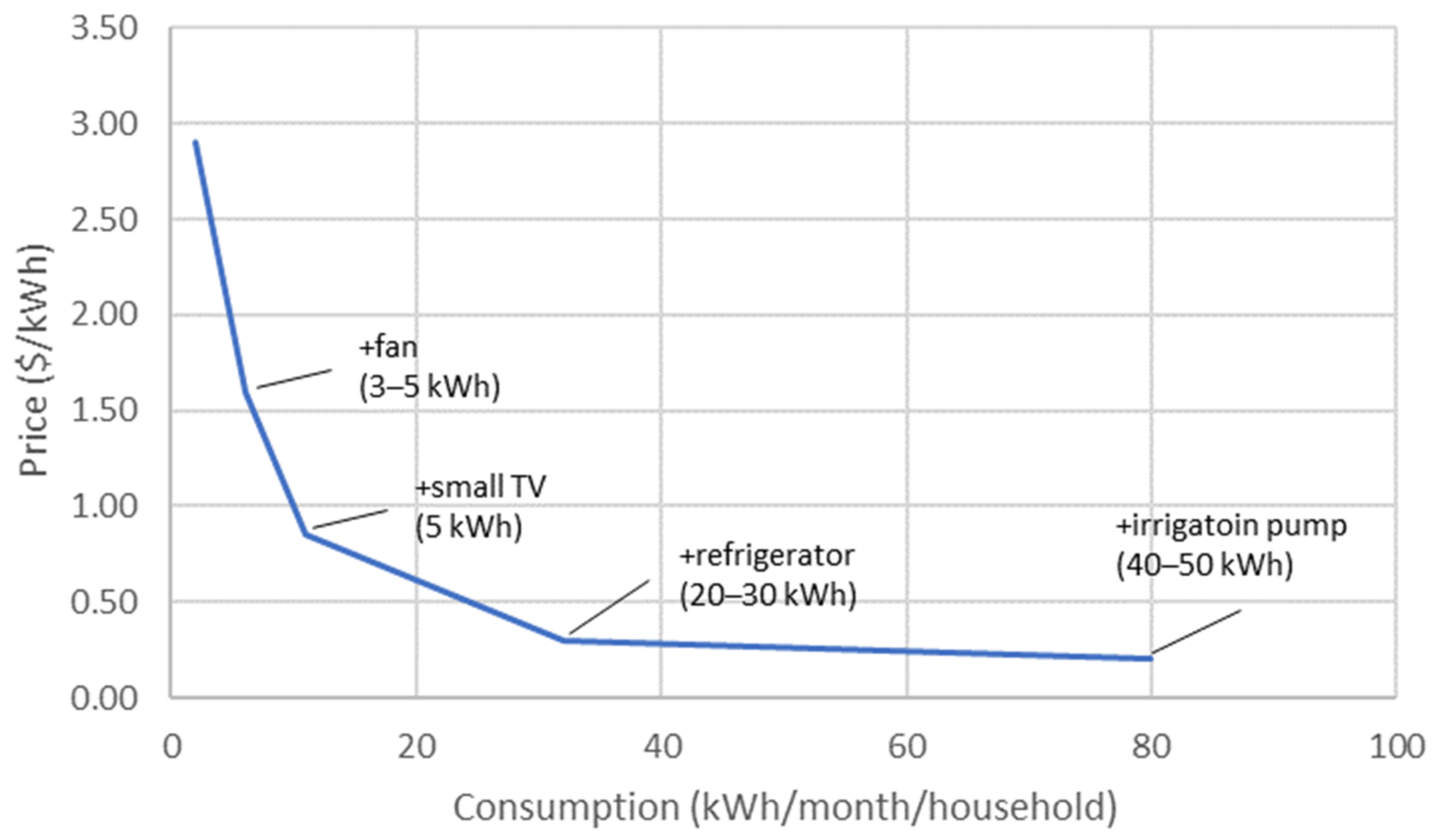
Households in underserved, rural areas tend to be poor, so the amount of disposable income they have available to spend on electricity is low. Average revenue per user (ARPU) tends to be low, yet this is a key metric for attracting project finance [5]. ARPU is a product of the amount of electricity used and the tariff charged so both aspects are of interest. Of course, they are intrinsically linked, such that consumption will increase as tariffs drop and vice versa, as illustrated in Figure 1. For example, the Access to Energy Institute (A2EI) have shown that use of electric pressure cookers (EPCs) on a mini-grid in Tanzania increased sharply when the tariff was reduced [6].

Solar photovoltaic (PV) has become the dominant energy generation technology deployed on mini-grids [5]. Solar resource is high and uniformly available across most developing country locations, making it widely applicable. The cost of PV panels has also dropped dramatically over recent years and is expected to continue to fall [5]. Advances in related technology such as batteries, control, and data analytics also contribute to falling mini-grid costs. Battery storage costs, in particular, play an important role in the financial viability of mini-grids, especially those based on intermittent renewable sources (e.g., solar, wind), and large-scale manufacturing is forecast to result in steep falls in energy storage costs up to 2030 [8]. However, items associated with generation (e.g., PV panels, batteries, inverters) typically account for only about half of total capex; the remainder is distribution network, metering, licenses, labor, taxes etc. [5].

The dynamic nature of loads affects the mini-grid system cost and the cost-recovery tariff. Along with system capacity (peak power) and the amount of electricity sold, key techno-economic considerations include capacity factor (energy sold as a proportion of total energy generation potential) and load factor (peak power demand as a proportion of average demand) [9]. Furthermore, the dynamic nature of loads throughout the day are especially important for mini-grids powered by intermittent energy sources, such as solar PV. Where energy demand takes place during daylight hours, when the solar resource is available, the need for energy storage is reduced, which reduces system capex costs [10]. For this reason, developers are keen to identify productive loads as anchor customers, given that businesses tend to operate during the daytime, giving a good match with energy production [11]. The most common types of load include services (e.g., barbers), small industry (e.g., welding, carpentry), agri-processing (e.g., milling), telecoms, and refrigeration [5]. Figure 1 illustrates how adding an agricultural load to a household can have a dramatic effect on the break-even tariff.

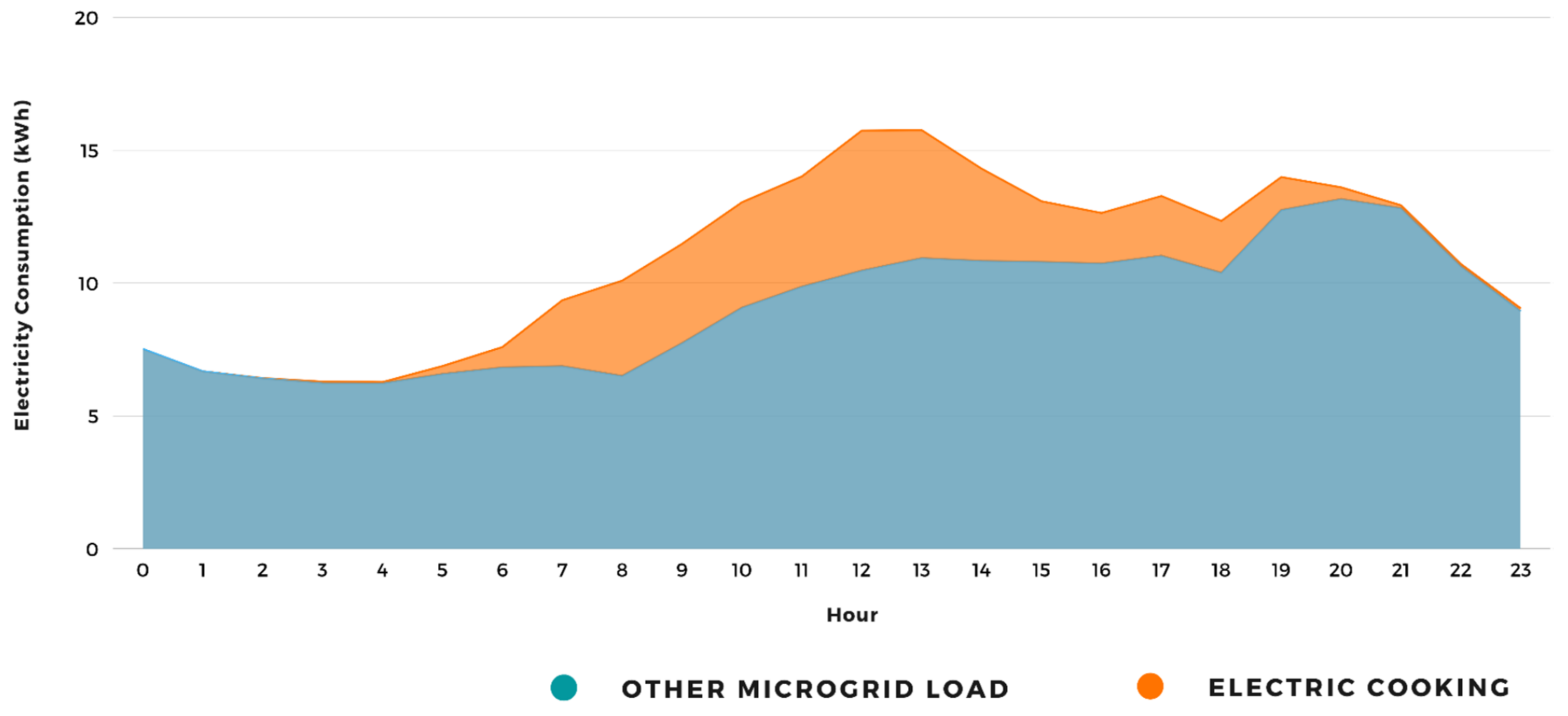
However, this literature misses the opportunity presented by electric cooking to increase demand. Moreover, in some countries, the main demand for cooking energy occurs in the middle of the day, making it an ideal load for solar PV mini-grids; Figure 2 presents an example from Haiti. However, recent studies have started to explore the cost implications of adding cooking loads to mini-grids. For example, Keddar et al. (2020) show that optimally sizing a PV battery system with diesel generator backup to meet cooking loads on a mini-grid can reduce the cost of energy by 70% (from 1.47 USD/kWh to 0.43 USD/kWh) [12].

Understanding consumer loads is a crucial part of mini-grid system design [14,15]. Overestimating loads means that a system will be oversized, so capital expenditure will be unnecessarily high and revenues less than expected. Conversely, underestimating loads means that a system will not have the capacity to meet demand, leading to poor customer satisfaction. Accurate estimation of consumer loads is therefore important, but many mini-grid installations target consumer groups which have had limited or no previous access to electricity, making estimation challenging [16]. Mandelli et al. [17] briefly overview commonly used techniques that generate load profiles for a given mini-grid (the characterization of variation in electricity consumption over time) by using a combination of load profiles from similar contexts and household surveys [18,19]. Recently, academics including Mandelli et al. have also developed software which attempt to generate these profiles using mathematical models [20,21,22].

These approaches rely on load profiles from consumer groups in similar contexts to the mini-grid in question, but data from low income households in Africa are lacking. Lorenzoni et al. (2020) identify a few initiatives gathering data on load profiles before conducting an analysis of 66 load profiles from around the world [23]. One exception is the South African Electrical Load Study data [24], although this may have limited applicability to the rest of sub-Saharan Africa.

In the absence of load profile data, developers tend to resort to surveys as the best way of estimating potential demand. Load profiles can then be generated from estimates of appliances and power ratings, coupled with time of day patterns of use. One study that conducted both surveys and subsequent electrical monitoring showed distinct differences between load profiles based on interviews and measured data (mainly during the night and in morning usage) [18], underlining the importance of publicly available data on load profiles. This paper makes a contribution to filling this gap by presenting load profile data from mini-grids in Tanzania. It complements data from similar sites in Tanzania [25] in a study that explored the use of demographic variables as predictors of customer type.

The same team has published further work demonstrating how mini-grid customers in Tanzania can be divided into five distinct load profile types [26]. This kind of customer segmentation, based on clustering techniques, is important to energy utilities more widely and can be used, for example, for energy efficiency campaigns, pricing, energy forecasting, and distributed generation planning [24].

In the absence of comprehensive data on electrical consumption characteristics of mini-grid customers in low income countries, developers resort to modelling for the purposes of system sizing and financial assessment. The paper presents load profile data from mini-grids in Tanzania. In order to inform modelling approaches, the analysis provides some understanding of the factors that lie behind electrical load profiles exhibited by different groups of mini-grid customers.

2. Methods and Data

2.1. Methods

The paper is based on electricity consumption data combined with customer data (demographic and asset ownership). Metered electricity consumption data for mini-grid customers were provided by PowerGen Renewable Energy. Customer data were generated from household surveys conducted through face to face interviews implemented by the Modern Energy Cooking Services (MECS) program. Both sets of data were generated as part of a broader study initiated by A2EI.

The pilot study in six mini-grid sites in northern Tanzania set out to explore whether EPCs are socially acceptable and useful, and technically and financially viable, as a clean cooking solution for mini-grid customers. The study was conducted in collaboration with Nexleaf Analytics, PowerGen, and the MECS program. Under the study, a total of 100 households from across all six sites were equipped with EPCs. A subset of households drawn from only two sites were recruited into a detailed study, which included the customer data survey.

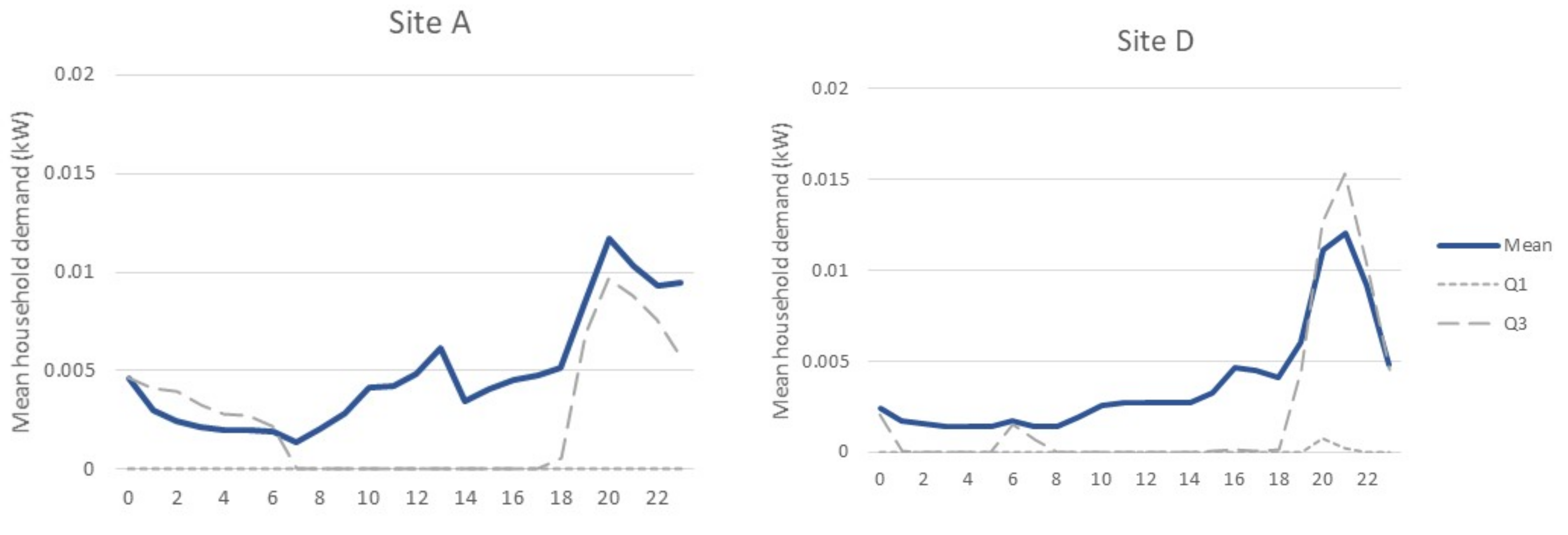
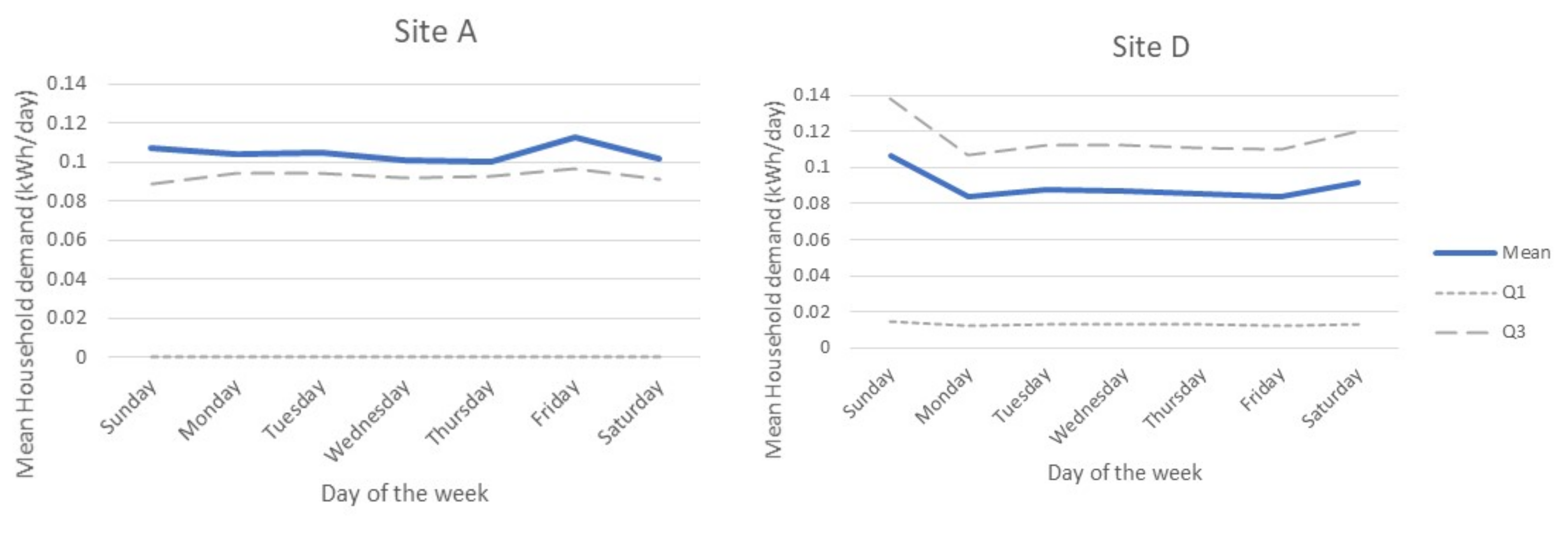
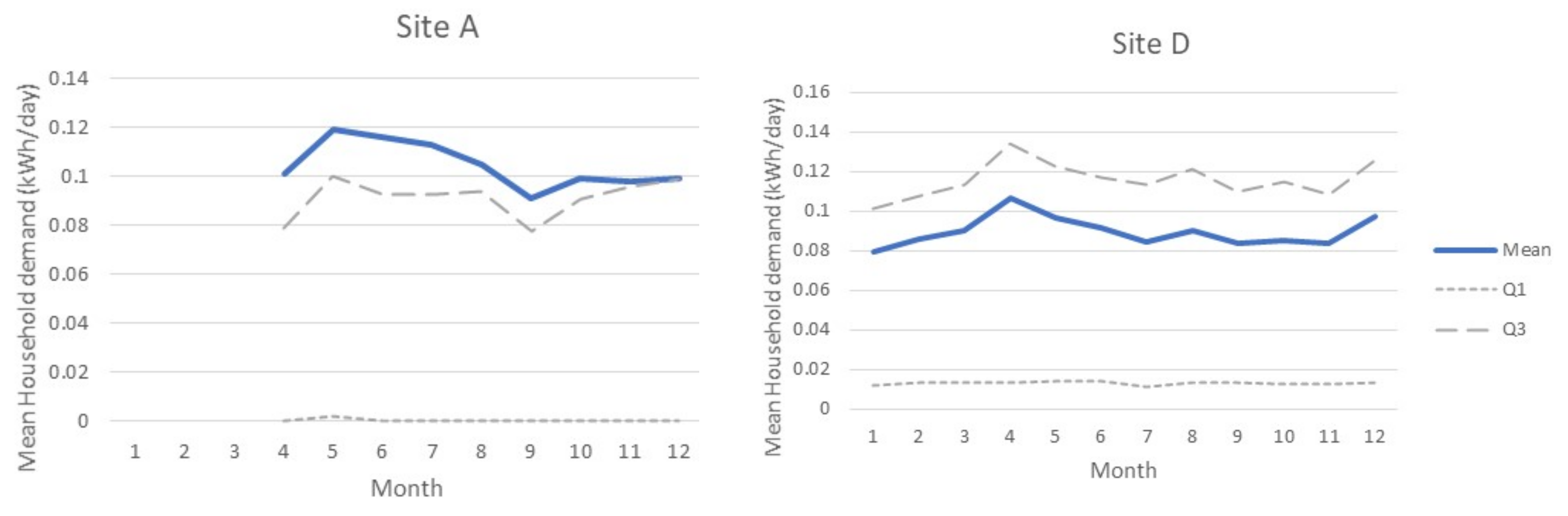
The analysis starts in Section 3 by considering demand across all customers in the two sites of interest, looking at variations across the day (24 h profiles), across the week (by day of the week), and seasonally (by month). It then moves on to considering the daily consumption and links to both demographics and electrical asset ownership using variables collected for the detailed study sample only (35 households). In Section 5, the 35 households are categorized according to the shape of their 24 h load profile using a k-means clustering algorithm. Both demographic and electrical asset variables are disaggregated by load profile category to explore factors lying behind the different profile shapes. The analysis was carried out using SPSS.

2.2. Description of Datasets

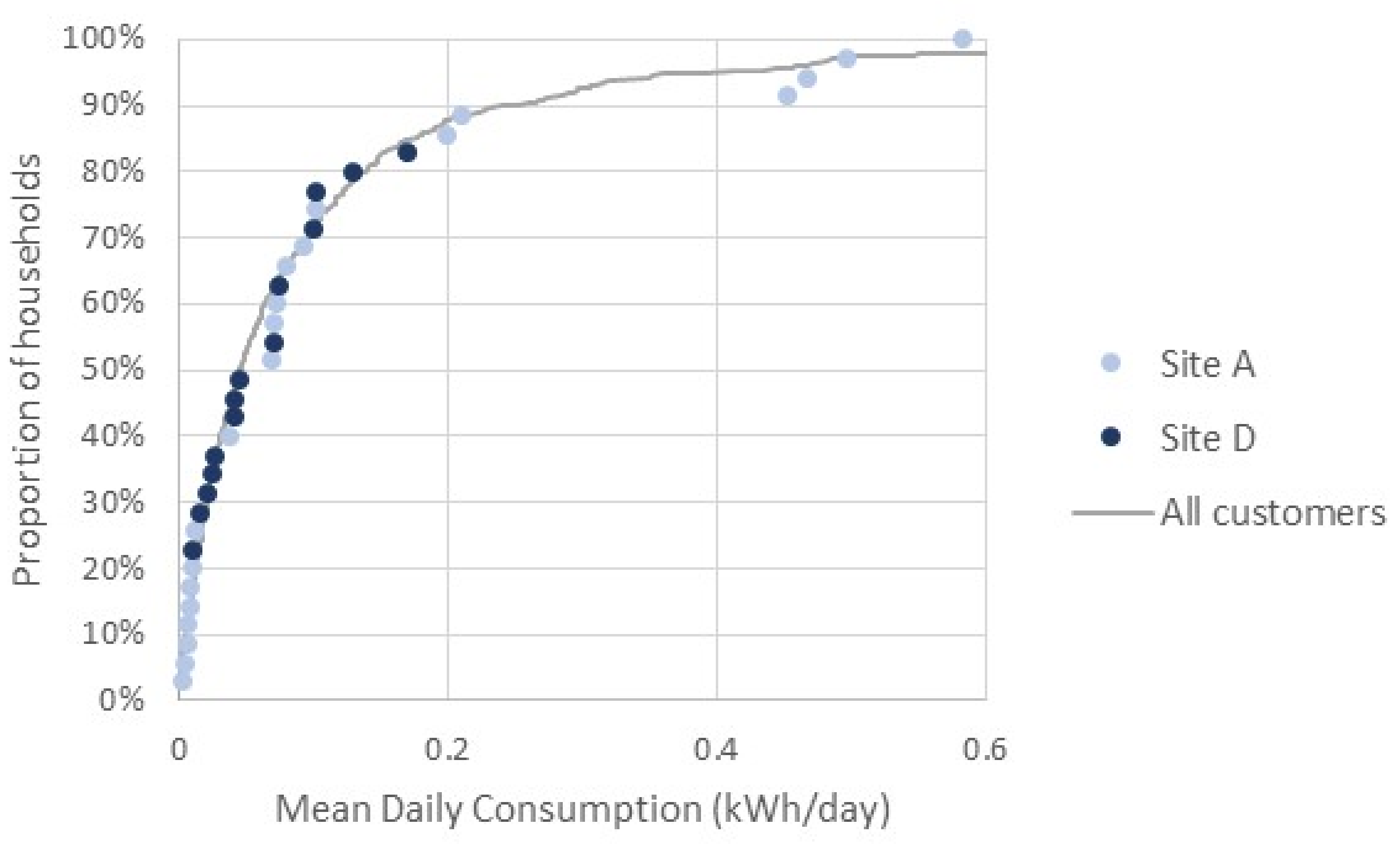
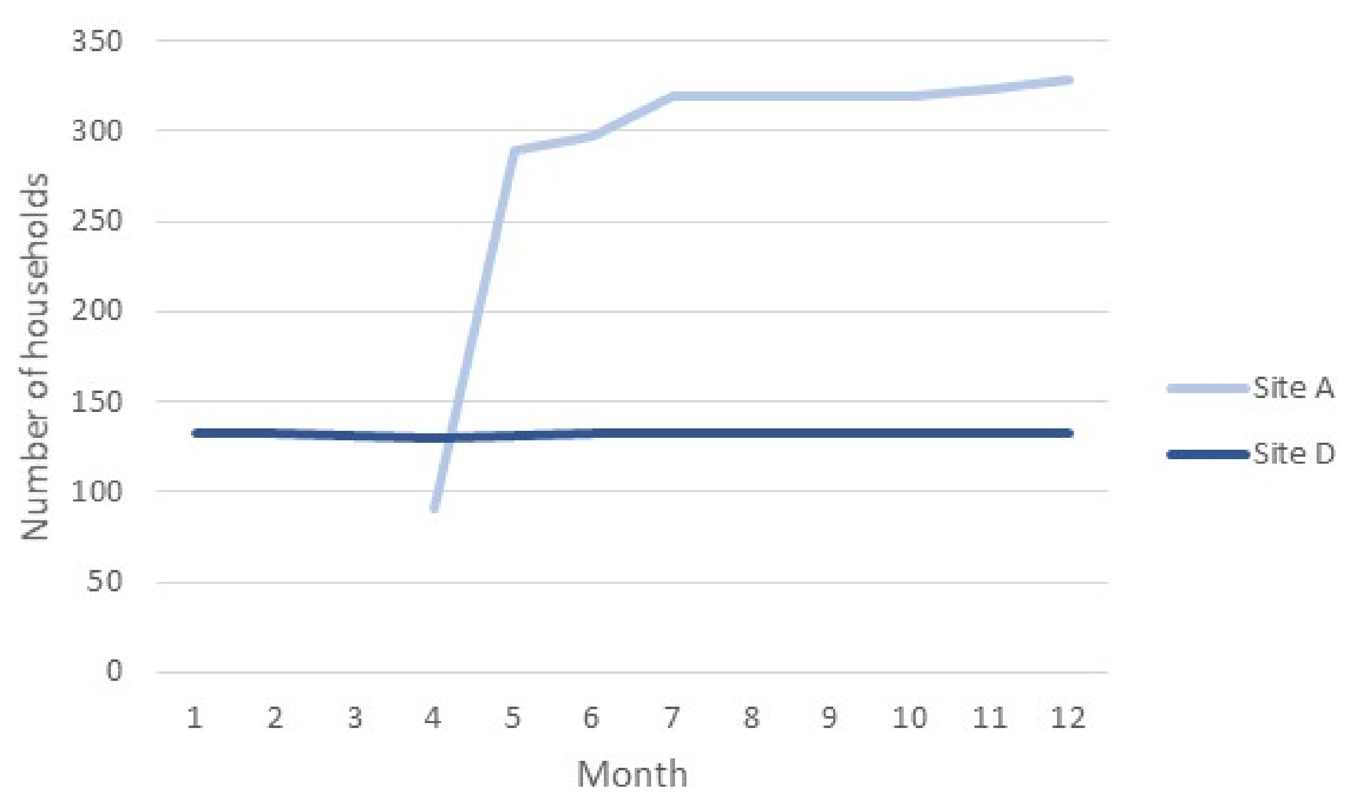
The two sites were chosen to reflect the diversity of communities served by PowerGen mini-grids. Site A is an island community, poor and isolated with buildings arranged at high density. Site D is a small rural village on the mainland, more spread out in terms of placement of houses and shops. It is the central village to six smaller sub-villages, two of which are also connected to the mini-grid.

Tariffs on these mini-grids were high relative to the national grid. Customers on the island site (Site A) were charged a flat tariff (independent of consumption) and mainland customers (Site D) were charged a block rate tariff, attracting a 37.5% discount if they used at least 3 kWh in a month. These sites have mixed generation (solar PV with battery storage and diesel backup) designed to have adequate capacity to meet demand so customers were not restricted as to the electrical devices they could use.

Electrical load data (hourly frequency) provided covered the period from their introduction to the community up to the end of 2019.

• Site A: 1,735,779 records; April–December 2019;
• Site D: 2,029,135 records; March 2018–December 2019.

For each site, these records comprised the following data:

• Time stamp;
• Customer meter number;
• Energy consumption (in the hour) (kWh).

For the purposes of this analysis, the hourly meter data were aggregated into a wide format, in which each record represented a single day, with 24 variables containing the energy consumption data for each hour of the day. Note that some readings were missing from the meter dataset, so the analysis has been conducted only on those records containing a full set of 24 hourly values. The analysis is based on 12 months of metering data for Site D covering all of 2019, and eight months of data for Site A covering May to December 2019.

Researchers from the University of Strathclyde (part of the MECS team) had developed a survey tool under a different cooking related program [27]. For the purposes of the detailed study of a sub-set of households, the survey was adapted to gather data on electrical household assets. It also included a series of poverty assessment questions following the PPI methodology, both of which are of value to this study. The survey was conducted in June 2020. The household survey data were gathered from 42 households from both Site A and Site D via face-to-face interviews with adult respondents, usually the female spouse of the household head. Thirty-five surveys could subsequently be paired with PowerGen meter numbers for which there were valid electrical metering data (21 households from Site A and 14 from Site D).

Load profile data are presented for all households in each of the two sites in Section 3. The rest of the analysis has been conducted on the 35 households from the detailed study sample for which electricity metering data were available. The demographic and asset data for each customer were merged into each complete 24 h load profile data record. The number of households and the number of complete 24 h load profiles used in the analysis are presented in

Table 1. Summary of data sets.

		Site A	Site D	Total
Pilot study	Number of customers (households)	358	135	493
Detailed survey	Household surveys (households)	21	14	35
	Complete 24 h load profiles	3824	4717	8541

.

2.3. Household Demographics

All respondents to the household survey were women apart from two men, both from Site D.

Site A had a much wider range of age of respondents, and the mean age of respondents was higher (39 years old compared with 32 years for Site D). The majority of respondents from Site D were aged 30–34 years.

Respondents from Site A had attained a higher level of education than those from Site D (

Table 2. Highest level of education attained by respondents.

Highest Level of Education	Site A	Site D
None	1	0
Form 3–4	4	5
Std 5–8	16	9
Total	21	14

).

With an average household size of 5.3, households from Site A were marginally smaller than those from Site D (average of 5.7).

The survey included a range of variables used to construct a PPI score in accordance with the Poverty Probability Index methodology [28]. The PPI methodology uses 10 questions on household characteristics and asset ownership to assess the probability of a household living below the national poverty line. Higher scores reflect a higher probability of being below the poverty line, so higher scores represent poorer households. Scores indicate that households from Site A have a higher probability of being below the national poverty line (6.2%) than those from Site D (3.7%).

3. Load Profiles

3.1. Sites and Demand Profiles

Site A came online during 2019, whereas Site D has been operational for longer, having been set up in early 2018. Despite being younger, Site A has attracted nearly three times as many customers as Site D (

Table 3. Comparison of sites (all customers).

	Total Energy Supplied (kWh)	Number of Households *	Daily Household Consumption (kWh/day/hhold)
			Mean	Std.dev.
Site A	8300 (9 months)	358	0.104	0.262
Site D	4300	135	0.089	0.134

* This is the total number of discrete accounts (serial numbers) with records in 2019. The total number of households on a mini-grid network at any given time will be less than this, as households drop off and others join.

). Note that the mean daily consumption for both sites is similar. Figure 3 shows that once customers are connected (within a few months), the number of customers remains constant, with little further growth. However, it appears that some households have also dropped off the system—Site A includes 358 accounts, but there were only 329 households with data in December 2019.

A comparison of mean hourly consumption for each site is presented in Figure 4. This shows a good deal of similarity across the two sites, with load gradually building throughout the day and a clear peak in the evening. For both sites, even the third quartile remains at zero for much of the day, indicating only a small proportion of customers account for much of the demand reflected in the mean lines. Eight percent and sixteen percent of customers in Site A and Site D, respectively, account for half of the metered energy delivered. This effect can also be seen in the distribution of daily consumption figures in Figure 7.

3.2. Variation in Demand (Daily and Seasonal)

Figure 5 indicates that whereas daily consumption is fairly constant in Site A, daily consumption in Site D tends to increase slightly on weekends (Saturday and Sunday).

The limited amount of data presented in Figure 6 suggests that there is a weak seasonal trend of declining consumption over half of the year (from May to November) before demand picks up at the end of the year. Demand is approximately 20% lower during low consumption months than at peak demand.

4. Energy Consumption Patterns

4.1. Daily Energy Consumption

The mean daily energy consumption for households enrolled in the detailed study in each site are presented in

Table 4. Mean daily electricity consumption by site—detailed study sample and entire site.

	Detailed Study Sample				Entire Site
	Number of Households	Number of Complete Load Profiles *	Daily Household Consumption (kWh/day/hhold)		Number of Households	Daily Household Consumption (kWh/day/hhold)
			Mean	Std.dev.		Mean	Std.dev.
Site A	21	3824	0.143	0.230	358	0.104	0.262
Site D	14	4717	0.062	0.072	135	0.089	0.134

* Days with complete set of readings.

. Note that mean consumption across all households in Site A is roughly twice that of households in Site D. This implies that demand among the households enrolled in the detailed study in Site A is higher than the site average, and demand among households enrolled in Site D is below the site average (consumption for all households in each site is presented in Table 3). There are a few households in Site A with high levels of demand. Figure 7 shows an even distribution of demand up to around 0.1 kWh/day and that 80% of households have a demand less than this figure. The remaining households have substantially higher levels of demand. The chart includes a line that represents the distribution of loads among all customers in the PowerGen dataset (493 households), which shows the same characteristics. The figure also shows a wide range of household consumption in Site A, as a cluster of households with the lowest demand and a cluster of households with highest demand around 0.5 kWh/day are all in Site A.

4.2. Influence of Demographic Factors

There is little evidence that consumption is higher among better educated respondents (

Table 5. Mean daily energy consumption by respondent’s level of education.

Highest Level of Education (Respondent)	Number of Households	Mean Daily Household Consumption (kWh/day/hhold)
None	1	0.003
Form 3–4	9	0.182
Std 5–8	25	0.090
Total	35	0.111

). Younger customers tend to use more electricity (

Table 6. Mean daily energy consumption by respondent’s age group.

Age Group (Respondent)	Number of Households	Mean Daily Household Consumption (kWh/day/hhold)
<30	5	0.170
30–39	19	0.112
40+	11	0.082
Total	35	0.111

).

The mean daily consumption for each of the 35 households is plotted against household size in Figure 8. Although the figure suggests that consumption may be higher among larger households, the correlation is not significant.

Similarly, there is no clear evidence that consumption is lower among poorer households. For the 35 households, the correlation between PPI score and consumption is not significant.

4.3. Ownership of Assets

The number of electrical assets owned by each household is presented in Appendix A. Households in this table are ranked by the mean daily household consumption; there is no obvious link between electricity consumption levels and electrical asset ownership. Consumption is of course somewhat dependent on electrical assets owned by the household, but both ownership and the extent to which assets are used will be a function of disposable income (wealth). Using the PPI poverty ratings as a measure of wealth,

Table 7. Link between electrical asset ownership and poverty (more than 3 items owned—detailed study households).

Electrical Asset	Ownership (A Binary Indicator of Ownership (y/n); Does Not Take into Account the Number of Working Assets Owned) and PPI Scores (Means)				Significance p-Value *
	Yes		No
	(n)	Probability of Poverty	(n)	Probability of Poverty
Mobile	32	4.8%	3	9.1%	0.062
Radio	19	3.9%	16	6.7%	0.502
TV	21	2.4%	14	9.4%	<0.001
Battery Torch	7	3.6%	28	5.6%	0.3
Fixed Lighting	12	3.8%	23	5.9%	0.263

* p-value of Mann–Whitney test.

shows that, among the small sample of 35 households, TVs are the only asset for which ownership can be shown to be linked to the poverty status of the household. This is to be expected, because TV ownership is one of the indicators used in calculating PPI scores.

5. Patterns of Use

5.1. Categories of Consumption Profiles

The bottom-up approach to modelling demand requires estimating hours of use for each electrical asset allocated to different customer segments. This section clusters households according to their load profiles in order to identify distinct patterns of use, which can then be used for modelling purposes.

The data show that for most households, there are a small number of high hourly meter readings, which may reflect exceptional household activity, or may reflect an anomaly in the metering (see Figure 9 for an example). Either way, these can have a substantial effect on mean hourly consumption values. For the purposes of constructing load profiles, modelers are more interested in “typical” patterns of consumption, so median hourly consumption figures have been used for the following clustering exercise.

Cumulative demand patterns have been calculated for each of the 35 households of interest. For each household, daily cumulative profiles have been created by summing consumption throughout the day. Normalized cumulative profiles were calculated for each household on each day by dividing each cumulative hourly consumption figure by the total consumption for the day. Normalized median hourly cumulative demand curves have been created for each household based on the median value of the normalized cumulative consumption at each hour of the day. When households have been grouped together, load profile curves have been based on the median values of the normalized median hourly cumulative demand values. (Because using median values has eliminated the effect of outliers, there is little difference between using mean or median values when grouping households.) The profile for all households in the detailed study (Figure 10) shows minimal consumption at night, demand building gradually throughout the day, and a peak in the evening. The variability across households is represented by the interquartile range shown on this chart. It is this variability that can be used to categorize customers according to their different load profile shapes.

In order to break households down into groups with different patterns of consumption, the 24 h normalized cumulative load values were clustered using the commonly used k-means algorithm (using SPSS) (e.g., Williams et al., 2018). Four clusters have been selected, as each appears to give a distinct usage profile, as illustrated in Figure 11 and summarized in

Table 8. Visualize patterns of use by cluster.

Group	Night	Day	Evening
24 h
Eve and night
Eve peak
Day and eve

Shaded cells represent main periods of electricity demand.

. These clusters, or groups of households, reflect different patterns of use:

• 24 h—constant during night and day, peak in evening (9 households);
• Eve and night—on in evening and night, minimal during day (7 households);
• Eve peak—off during night and day, peak in evening (11 households);
• Day and eve—off at night, on during day, peak in evening (8 households).

5.2. Characteristics of Groups

The clustering of households is based entirely on the shape of demand profiles, as it is based on normalized consumption figures. Therefore, it tells us nothing about actual energy consumption. The consumption figures in

Table 9. Mean daily consumption by group.

Group	Number of Complete Load Profiles	Daily Consumption (kWh/day)
		Mean	Std.dev.
24 h	2165	0.212	0.257
Eve and night	1447	0.124	0.148
Day and eve	1879	0.052	0.072
Eve peak	3050	0.033	0.055
Total	8541	0.098	0.168

show that consumption is highest among the ‘24 h’ group (households that use electricity throughout the day and night), and lowest among the ‘Eve peak’ group (households that only use electricity during a short peak in the evening). Note that the ‘Eve and night’ group is drawn mostly from Site A (

Table 10. Distribution of groups across sites.

Group	Site A	Site D	Total
24 h	6	3	9
Eve and night	6	1	7
Eve peak	5	6	11
Day and eve	4	4	8

).

There is no obvious link between load profiles and the number of children in the household (

Table 11. Household size (means) by pattern of use groups.

Group	Adults	Children	Household Size
24 h	2.5	2.7	5.2
Eve and night	3.3	3.0	6.3
Eve peak	2.2	2.9	5.2
Day and eve	2.8	3.5	6.2
Total	2.6	3.0	5.6

). For example, having children in the household could be expected to give rise to demand during the day, as in the 24 h group, but all of the groups have roughly the same number of children, so children do not appear to be causing differences in profiles. Similarly, the total number of people in the household does not appear to explain differences in profiles.

Although

Table 12. Poverty (probability of being below the national poverty line—means) by pattern of use group.

Group	Number of Complete Load Profiles	Probability of Poverty (PPI)
24 h	2165	2.6%
Eve and night	1447	9.4%
Eve peak	3050	4.1%
Day and eve	1879	5.3%
Total	8541	4.9%

shows that households in the ‘Eve and night’ group are poorer than those in the other groups, consumption among these households is far from the lowest (see Table 9). Note that this profile is characterized by high nighttime usage (Figure 11), which may, for example, reflect security concerns and the use of security lighting throughout the night. The ‘24 h’ group has the lowest incidence of poverty, and has the most uniform profile, indicating that electricity is used throughout the night and daytime, and then consumption increases during the evening. Although the number of households in the sample is small, and differences in poverty status between groups are modest; this suggests that the different patterns of use can be related to poverty, but not necessarily as might be expected (i.e., the poorest group exhibits demand at night and has relatively high levels of consumption).

5.3. Linking Assets to Electricity Consumption

Household asset ownership has been separated out into the patterns of use groups in

Table 13. Mean number of assets per household in each group.

Group	Mobile	Fan	Radio	Stereo	Fridge	TV	Rechargeable Torch	Battery Powered Torch	Fixed Lighting
24 h	3.9	0.0	1.0	0.1	0.3	0.9	0.1	0.6	0.9
Eve and night	1.7	0.0	0.4	0.0	0.0	0.4	0.0	0.0	0.9
Eve peak	1.5	0.0	0.3	0.0	0.0	0.5	0.0	0.4	0.8
Day and eve	2.4	0.1	0.6	0.0	0.0	0.6	0.0	0.0	1.3

. A visual assessment of the mean number of assets held by households in each group suggests that:

• The ‘24 h’ group is relatively asset-rich.
• The ‘Eve peak’ group is relatively asset-poor.

This is not entirely consistent with the poverty ratings in Table 12, but it is consistent with the mean electrical consumption figures in Table 9. This simply confirms that electricity consumption is linked to asset ownership, albeit weakly.

Each of the patterns of use groups represent different ways in which people use the appliances in their households. The correlations presented in

Table 14. Correlation of daily consumption (kWh) with number of assets by group (correlation coefficients).

	24 h	Eve and Night	Eve Peak	Day and Eve
Mobile		−0.225 ***		0.657 ***
Fan
Radio		−0.226 ***
Stereo
Fridge	0.251 ***
TV	0.297 ***	0.505 ***	0.308 ***
Rechargeable Torch	0.283 ***
Battery Powered Torch
Fixed Lighting	−0.232 ***	0.731 ***	0.295 ***	−0.256 ***

*** Correlation is significant at the 0.001 level.

show the extent to which, within each group, the number of appliances owned is linked to energy consumption.

The highest energy consuming appliances are likely to be TVs and fridges, and these consistently correlate with daily energy consumption across most groups. Note that only two households have a fridge (both in the 24 h group), one of which owns two fridges that are used for a business selling drinks; nighttime demand among this group is lower than might be expected because the drink fridges are turned off at night to save money. Many of the linkages in Table 14 are counterintuitive, as negative correlation coefficients suggest that energy consumption decreases with more devices in the household. This reflects appliances for which the patterns of use can be the dominant factor in determining energy consumption rather than the number of appliances.

6. Conclusions

Load profiles from the two communities demonstrate four distinct patterns of use based on the shape of the load profiles. All households exhibited a peak in demand during the evening; two groups exhibited demand throughout the night, and two exhibited demand throughout the day. One possible explanation is that these patterns of use reflect different occupancy schedules. In addition to demographic data, this paper has also analyzed data on household electrical asset ownership in exploring linkages with these patterns of use.

The results show that patterns of use depend on a complex mix of factors:

• Load profiles can be linked to poverty, but not necessarily as might be expected. For example, some low-status households use electricity throughout the night, which contributes to relatively high consumption figures. This may reflect security concerns, but this would need further investigation. Conversely, other households that have a reasonable mix of appliances but use them sparingly, resulting in low levels of electricity consumption, have a relatively low probability of being poor.
• Asset ownership and electricity consumption are not necessarily linked to socio-economic status. For example, the group with the lowest level of electricity consumption are relatively asset-poor, but are far from the poorest households. On the other hand, high-cost items, which also have high power ratings (notably fridges and TVs), are more frequently found in households with high levels of electricity consumption that exhibit demand throughout the 24 h period and also have a higher socio-economic status.
• Asset ownership is linked to electricity consumption, albeit weakly. The group with highest electricity consumption has the highest levels of asset ownership, whilst the group with lowest consumption is relatively asset-poor. Ownership of assets with high power ratings, such as fridges and TVs, are linked with higher electricity consumption, but this is not necessarily the case for other appliances.
• With appliance ownership and poverty showing relatively weak relationships with energy consumption, it is proposed that patterns of use based on occupancy can be the dominant factor in determining energy consumption rather than the number of appliances, e.g., demand among working households could be lower during working hours. However, occupancy cannot fully explain profiles. For example, some households use electricity at night while others do not, yet it can be assumed that most households will be occupied at night.
• Patterns of use are not linked to household composition. There is no clear link with the number of children in the household, and household sizes are similar across all groups.

The distinct shapes of load profiles for each of the groups highlight the importance of understanding patterns of use for modelling. When coupled with energy consumption data, this can be used not only for customer segmentation, but also for system sizing according to demand variation throughout the day.

The paper makes a contribution to understanding the composition of electrical appliances within households with different load profile characteristics, and the interdependence between appliances and load profiles. It demonstrates that different load profiles are determined by a complex mix of appliance ownership, occupancy, and socio-economic status. In order to further test the role of occupancy in load profiles, the MECS program will be gathering household occupancy data as part of ongoing studies.

References

1. ESMAP. SDG7: Tracking the Energy Progress Report 2020; ESMAP: Washington, DC, USA, 2020. [Google Scholar]
2. IEA. The Covid-19 Crisis Is Reversing Progress on Energy Access in Africa. Available online: https://www.iea.org/articles/the-covid-19-crisis-is-reversing-progress-on-energy-access-in-africa (accessed on 3 June 2021).
3. IRENA. Off-Grid Renewable Energy Solutions; IRENA: Abu Dhabi, United Arab Emirates, 2018. [Google Scholar]
4. IEA. Africa Energy Outlook 2019; IEA: Berlin, Germany, 2019. [Google Scholar] [CrossRef] [Green Version]
5. Sustainable Energy for All. State of the Global Mini-Grids Market Report 2020; Sustainable Energy for All: Washington, DC, USA, 2020. [Google Scholar]
6. A2EI. A2EI Clean Cooking Data Release the Future of Clean Cooking; A2EI: Bourgogne, France, 2020. [Google Scholar]
7. Institute for Transformative Technologies (ITT). Achieving Universal Electrification in India. A Roadmap for Rural Solar Mini-Grids; Institute for Transformative Technologies: Berkeley, CA, USA, 2016. [Google Scholar]
8. IRENA. Renewable Mini-Grids: Innovation Landscape Brief; IRENA: Abu Dhabi, United Arab Emirates, 2019. [Google Scholar]
9. Hartvigsson, E.; Ehnberg, J.; Ahlgren, E.O.; Molander, S. Linking Household and Productive Use of Electricity with Mini-Grid Dimensioning and Operation. Energy Sustain. Dev. 2021, 60, 82–89. [Google Scholar] [CrossRef]
10. Moner-Girona, M.; Solano-Peralta, M.; Lazopoulou, M.; Ackom, E.K.; Vallve, X.; Szabó, S. Electrification of Sub-Saharan Africa through PV/Hybrid Mini-Grids: Reducing the Gap between Current Business Models and on-Site Experience. Renew. Sustain. Energy Rev. 2018, 91, 1148–1161. [Google Scholar] [CrossRef]
11. Contejean, A.; Verin, L. Making Mini-Grids Work: Productive Uses of Electricity in Tanzania; International Institute for Environment and Development: London, UK, 2017. [Google Scholar]
12. Keddar, S.; Strachan, S.; Eales, A.; Galloway, S. Assessing the Techno-Economic Feasibility of ECook Deployment on a Hybrid Solar-Diesel Mini-Grid in Rural Malawi. In Proceedings of the IEEE PES/IAS Power Africa 2020, Nairobi, Kenya, 25–28 August 2020; pp. 1–5. [Google Scholar] [CrossRef]
13. Bilich, A.; Sanassee, W.; Archambault, A.; Eberwein, A.; Thaylord, J. Kwison Elektrik. Solar Power for Electricity Access and Electric Cooking in Haiti; Earthspark International: Washington, DC, USA, 2021. [Google Scholar]
14. Louie, H.; Dauenhauer, P. Effects of Load Estimation Error on Small-Scale off-Grid Photovoltaic System Design, Cost and Reliability. Energy Sustain. Dev. 2016, 34, 30–43. [Google Scholar] [CrossRef] [Green Version]
15. Mandelli, S.; Brivio, C.; Colombo, E.; Merlo, M. Effect of Load Profile Uncertainty on the Optimum Sizing of Off-Grid PV Systems for Rural Electrification. Sustain. Energy Technol. Assess. 2016, 18, 34–47. [Google Scholar] [CrossRef]
16. Gambino, V.; Del Citto, R.; Cherubini, P.; Tacconelli, C.; Micangeli, A.; Giglioli, R. Methodology for the Energy Need Assessment to Effectively Design and Deploy Mini-Grids for Rural Electrification. Energies 2019, 12, 574. [Google Scholar] [CrossRef] [Green Version]
17. Mandelli, S.; Merlo, M.; Colombo, E. Novel Procedure to Formulate Load Profiles for Off-Grid Rural Areas. Energy Sustain. Dev. 2016, 31, 130–142. [Google Scholar] [CrossRef]
18. Hartvigsson, E.; Ahlgren, E.O. Comparison of Load Profiles in a Mini-Grid: Assessment of Performance Metrics Using Measured and Interview-Based Data. Energy Sustain. Dev. 2018, 43, 186–195. [Google Scholar] [CrossRef]
19. Blodgett, C.; Dauenhauer, P.; Louie, H.; Kickham, L. Accuracy of Energy-Use Surveys in Predicting Rural Mini-Grid User Consumption. Energy Sustain. Dev. 2017, 41, 88–105. [Google Scholar] [CrossRef] [Green Version]
20. Boait, P.; Advani, V.; Gammon, R. Estimation of Demand Diversity and Daily Demand Profile for Off-Grid Electrification in Developing Countries. Energy Sustain. Dev. 2015, 29, 135–141. [Google Scholar] [CrossRef] [Green Version]
21. Narayan, N.; Qin, Z.; Popovic-Gerber, J.; Diehl, J.-C.; Bauer, P.; Zeman, M. Stochastic Load Profile Construction for the Multi-Tier Framework for Household Electricity Access Using off-Grid DC Appliances. Energy Effic. 2020, 13, 197–215. [Google Scholar] [CrossRef] [Green Version]
22. Leach, M.; Mullen, C.; Lee, J.; Soltowski, B.; Wade, N.; Galloway, S.; Coley, W.; Keddar, S.; Scott, N.; Batchelor, S. Modelling the Costs and Benefits of Moving to Modern Energy Cooking Services—Methods & Application to Three Case Studies; Working Paper; MECS: Loughborough, UK, 2021; Available online: https://mecs.org.uk/wp-content/uploads/2021/05/Modelling-the-costs-and-benefits-of-moving-to-Modern-Energy-Cooking-Services-%E2%80%93-methods-application-to-three-case-studies.pdf (accessed on 25 May 2021).
23. Lorenzoni, L.; Cherubini, P.; Fioriti, D.; Poli, D.; Micangeli, A.; Giglioli, R. Classification and Modeling of Load Profiles of Isolated Mini-Grids in Developing Countries: A Data-Driven Approach. Energy Sustain. Dev. 2020, 59, 208–225. [Google Scholar] [CrossRef]
24. Toussaint, W.; Moodley, D. Comparison of Clustering Techniques for Residential Load Profiles in South Africa. CEUR Workshop Proc. 2019, 2540, 117–132. [Google Scholar]
25. Otieno, B.; Williams, N.J.; McSharry, P. Customer Segmentation for East African Microgrid Consumers. In Proceedings of the IEEE PES/IAS Power Africa 2018, Cape Town, South Africa, 26–29 June 2018; pp. 468–473. [Google Scholar] [CrossRef]
26. Williams, N.J.; Jaramillo, P.; Campbell, K.; Musanga, B.; Lyons-Galante, I. Electricity Consumption and Load Profile Segmentation Analysis for Rural Micro Grid Customers in Tanzania. In Proceedings of the IEEE PES/IAS Power Africa 2018, Cape Town, South Africa, 26–29 June 2018; pp. 360–365. [Google Scholar] [CrossRef]
27. Coley, W.; Eales, A.; Frame, D.; Galloway, S.; Archer, L. A Market Assessment for Modern Cooking in Malawi. In Proceedings of the 2020 IEEE Global Humanitarian Technology Conference (GHTC), Seattle, WA, USA, 29 October–1 November 2020; pp. 1–8. [Google Scholar] [CrossRef]
28. Schreiner, M. PPI for Tanzania 2011. Available online: https://www.povertyindex.org/country/tanzania (accessed on 11 May 2021).
Figure 1. Break-even tariffs at different household electricity consumption levels. Authors’ own, drawn from [7].
Energies 14 04207 g001
Figure 2. Example of cooking and non-cooking loads on a mini-grid in Haiti (20 participants, month of October 2020) [13].
Energies 14 04207 g002
Figure 3. Growth in customer numbers (2019).
Energies 14 04207 g003
Figure 4. Hourly mean demand for each site.
Energies 14 04207 g004
Figure 5. Weekly trends in average daily household consumption.
Energies 14 04207 g005
Figure 6. Seasonal trends in average daily household consumption.
Energies 14 04207 g006
Figure 7. Cumulative curve of mean daily household demand (both sites).
Energies 14 04207 g007
Figure 8. Linkage between daily energy consumption and household size (35 households).
Energies 14 04207 g008
Figure 9. Hourly consumption (box and whisker plots)—Site D (all households).
Energies 14 04207 g009
Figure 10. Normalized cumulative load profile (35 households).
Energies 14 04207 g010
Figure 11. Normalized cumulative 24 h demand for groups (based on median hourly demand).
Energies 14 04207 g011