
Approximation of Hysteresis Changes in Electrical Steel Sheets


Department of Electrical Engineering, Cracow University of Technology, 31-155 Krakow, Poland
*
Author to whom correspondence should be addressed.
Energies 2021, 14(14), 4110; https://doi.org/10.3390/en14144110
Submission received: 23 May 2021
/
Revised: 29 June 2021
/
Accepted: 5 July 2021
/
Published: 7 July 2021
(This article belongs to the Section F: Electrical Engineering)
Abstract
:This paper describes a simple method of approximating hysteresis changes in electrical steel sheets. This method is based on assumptions that flux density or field strength changes are a sum or a difference of functions that describe one curve of the limiting hysteresis loop and a certain ‘transient’ component. Appropriate formulas that present the flux density as functions of the field strength and those that present inverse dependencies are proposed. An application of this approximation requires knowledge of the measured limiting hysteresis loop and a few minor loops. Algorithms for determining changes in the flux density or field strength are proposed and discussed. The correctness of the proposed approximation of hysteresis changes was verified through a comparison of measured hysteresis loops with the loops calculated for several different excitations of the magnetic field occurring in dynamo and transformer steel sheets. Additionally, an example of the application of the proposed approximation of hysteresis changes is discussed in the paper. The proposed approximation of hysteresis changes is recommended for numerical calculations of the magnetic field distribution in dynamo and transformer steel sheets.
1. Introduction
The hysteresis phenomenon is a characteristic feature of any magnetic circuit containing a ferromagnetic material. This phenomenon is related to a certain delay in changes in the magnetic flux density in relation to changes in the magnetic field strength in this material. The hysteresis mechanism is quite well known [1,2,3,4,5,6,7]; however, the formulation of an appropriate mathematical model based on the knowledge of the phenomena describing the magnetization process is still a complex issue. Therefore, for many decades, intensive research has been carried out to develop a hysteresis model that would be sufficiently accurate and useful in the field calculations of ferromagnetic materials.
On a micro scale, the study of magnetization processes is often based on the Landau–Lifschitz–Gilbert equation, which describes the behavior of a single magnetic dipole in an external magnetic field [4,5,6,8]. The original equation formulated by Landau–Lifschitz was modified by Gilbert to take into account the damping conditions of the magnetic moment rotation, which in the steady state will occupy a position along the direction of the magnetic field strength. As stated in a previous study [9], the calculation results obtained on the basis of the Landau–Lifschitz–Gilbert equation “can be averaged to provide hysteresis curves of material”. However, it should be mentioned that hysteresis curves of ferromagnetic materials are also often described by different empirical fitting procedures.
The best known models, which are based on energy relationships, are the Stoner–Wohlfarth and Jiles–Atherton models. The former presents the magnetization process as rotations of magnetic moments of non-interacting single-domain particles [10,11,12]. To take into account the interaction of particles, the concept of the effective field has been introduced, which is the sum of the field strength of the external magnetic field and the product of the magnetization and a certain dimensionless mean field parameter [4,8,10,11,12,13]. The resultant magnetization vector in the Stoner–Wohlfarth model is a sum of the magnetizations of single particles aligned along specified directions. However, displacements of the domain wall are not considered. The application of this model for macroscopic samples must specify a certain number of directions for a particular ferromagnetic material. Therefore, computation times are relatively long, and they depend directly on the number of specified directions.
The assumption that the energy supplied to a sample of an isotropic polycrystalline material is a sum of the change in the magnetostatic energy and hysteresis loss is the basis for the Jiles–Atherton model [5,9,11,12]. This model requires five physical parameters to describe hysteresis curves. However, in many instances, these parameters must be modified to obtain an effective representation of the measured waveforms. One difficulty is the determination of an anhysteretic curve because this curve is a theoretical curve. The Jiles–Atherton model is used in modelling relatively narrow hysteresis loops. Frequently, the model parameters should be determined for almost each amplitude of the field strength. This causes a certain inconvenience when using this model; nevertheless, this model and its modifications are still used [14,15,16,17,18,19,20,21,22,23,24,25].
The phenomenological Preisach model assumes that a considered ferromagnetic material consists of particles (hysterons), which are magnetized to a positive or negative saturation. A characteristic feature of this model is the Preisach triangle consisting of the following two parts: the first part refers to positively magnetized particles, and the second part refers to negatively magnetized particles. A certain distribution function, whose determination is time-consuming, describes how many hysterons are located at particular points of the Preisach triangle. This model enables the creation of any hysteresis or minor loop, depending on an appropriate distribution function. However, long calculation times and dependence on the degree of Preisach triangle discretization are significant disadvantages of this model. The Preisach model is still modified and often used in different applications [26,27,28,29,30,31,32,33,34,35,36].
Hysteresis models formulated with the use of special operators, the so-called ‘play’ and ‘stop’ hysterons, are also phenomenological [37]. These types of models were developed by Matsuo et al. [38,39,40,41]. Some hysteresis models are based on certain differential equations that relate the magnetic field strength to the magnetic flux density. However, these equations do not result directly from the mechanism of phenomena occurring in the magnetization process. The Hodgdon model belongs to this category [11,42]. The determination of functions occurring in the Hodgdon model is time-consuming and requires a series of tests. Note that slight changes in the parameters of these functions significantly affect the shape of the calculated hysteresis loops.
There are other, less known hysteresis models in the literature. One of them is the Globus model, which assumes that the behavior of the entire ferromagnetic sample can be reduced to one spherical grain [12]. This group also includes the hysteresis model developed by Chua [11]. In this model, the resultant magnetic field strength is the sum of the field strength resulting from the hysteresis-free magnetization curve and the field strength dependent on the derivative of the magnetic flux density versus time; in fact, the Chua model is a dynamic model. To describe changes in electrical steel sheets, the Pry and Bean domain model is also applied [43,44].
Calculations of the magnetic field distribution in electrical steel sheets often require consideration of the hysteresis phenomenon. These sheets are used in the construction of the magnetic cores of transformers, rotating machines, and other electrical devices. In many scenarios, a certain model of the hysteresis phenomenon must be considered when calculating the magnetic field distribution and hysteresis loss of a tested magnetic circuit. Instead of one unambiguous relationship, these models propose different dependencies between the flux density and field strength as the hysteresis changes. However, the formulation of a suitable mathematical hysteresis model based on the hysteresis mechanism is still a relatively difficult problem. Some magnetic hysteresis models refer to the so-called dynamic hysteresis loop, which considers the effects of eddy currents on changes in flux density. However, in many proposals, eddy currents are considered using separate differential equations [45,46].
It should be clearly emphasized that the purpose of this paper is not to formulate a new hysteresis model but rather to present a proposal for approximation of hysteresis changes; this approximation should be easily applicable to equations describing the magnetic field distribution. In calculations, the area of the magnetic field is divided into several dozen or even more thousand elementary segments. Owing to the nonlinear nature of electrical sheets, the magnetic flux density in individual segments changes in different ways. Therefore, the hysteresis phenomenon should be included in all elementary segments concerning a considered ferromagnetic material.
2. Approximation of Flux Density Changes
Each hysteresis model briefly discussed in the previous chapter has advantages and disadvantages. However, note that any model of the magnetic hysteresis should have the following properties:
- Easy determination of model parameters;
- Possibility of calculations for excitations using a constant component;
- Possibility of formulating an inverse model indicating the field strength as a dependence on the flux density;
- Relatively simple numerical algorithm;
- Short times for numerical calculations;
- Easy application of the selected hysteresis model to equations describing the magnetic field distribution.
Irreversible displacements of domain walls are the main cause of the hysteresis phenomenon in soft magnetic materials; these displacements are caused by changes in field strength in a sample of ferromagnetic materials. When the field strength values are low, then the magnetization process is reversible. However, for most soft ferromagnetic materials, particularly for electrical steel sheets, the effect of the reversible magnetization can be neglected. Notably, in a high-value range of the field strength, the magnetization process is also reversible, but then this process refers to reversible rotations of magnetization vectors towards the external magnetic field.
It follows from the nature of the hysteresis phenomenon that any point P with coordinates (H0, B0) inside the limiting hysteresis loop moves along a certain trajectory to the bottom or upper limiting curve depending on changes in the field strength (Figure 1). This means that the difference B0 − Bb(H0) between the initial flux density B0 at point P and the flux density value Bb(H0) on the bottom limiting curve determined for H0 should decrease to zero if the field strength H increases. Therefore, the difference B0 − Bb(H0) can be treated as an ‘initial value’ of the certain transient component of changes in the flux density of point P moving to the bottom limiting curve Bb(H).
In this paper, the subscripts B and H concern parameters which are related to changes in the flux density or magnetic field, respectively; subscripts b and u refer to the bottom or upper curve of the hysteresis loop, respectively, and the subscript r is used if the magnetic flux or field strength increases, otherwise the subscript d is used; for example, the parameter aBur relates to the case when the flux density B is a function of the field strength, u refers to the upper curve of the limiting hysteresis loop, and r is used when the flux density increases; in turn, the parameter aHbd relates to the case when the field strength H depends on the flux density, b refers to the bottom curve of the limiting hysteresis loop, and d is used when the field strength decreases.
Using some analogy to transient states occurring in electrical circuits, where the transient component of a certain quantity decreases and its changes are described by means of an exponential function, the flux density changes of point P(H0,B0) can be described as follows when the field strength H increases:
where Bb(H) is the bottom curve of the limiting hysteresis loop, ΔBr = B0 − Bb(H0), H0 and B0 denote the coordinates of point P(H0,B0), and kBr is an attenuation coefficient of the transient component when H increases.
The second component of Equation (1) is a certain pseudotransient component of the changes in flux density. The coefficient kBr(H) affects the ‘dynamics’ at which point P moves to the bottom limiting hysteresis curve. Generally, this coefficient is a nonlinear function of H.
When H decreases, the difference Bu(H0) − B0 between the flux density value Bu(H0) on the upper limiting curve, determined for H0, and the initial flux density B0 at point P should decrease to zero. Therefore, the difference Bu(H0) − B0 can be treated, similarly to previously, as a certain initial value of the transient component of changes in the flux density of point P moving to the upper limiting curve Bu(H). In this case, the change in the flux density Bd(H) of point P can be approximated as follows:
where Bu(H) denotes the upper limiting curve, ΔBd = Bu(H0) − B0, and kBd(H) is an attenuation coefficient of the transient component when H decreases.
Note that for decreasing values of the field strength H, the difference H-H0 is negative.
To apply this description of hysteresis changes, the limiting hysteresis loop must be measured for a considered electrical sheet. Here, when only the coercive field, residual flux density, and saturation flux density are known, curves of the limiting hysteresis loop can be approximated using, for example, an arctg function which considers the abovementioned parameters.
The coefficients kBr and kBd depend on the position of point P(H0,B0). Owing to the nature of the hysteresis phenomenon, the derivative dBr/dH on the trajectory of point P(H0,B0) for increasing values of H is in the range (aBur,aBbr), where aBur describes the value of this derivative when point P(H0,B0) is situated on the upper limiting curve Bu(H) (Figure 1), and aBbr denotes this derivative when point P(H0,B0) is situated sufficiently close to the bottom hysteresis curve, i.e., to the curve to which it moves when H increases. Thus, aBbr is equal to the derivative dBb/dH of the bottom curve at point Pr (Figure 1). The value aBur is determined based on several measured symmetrical hysteresis loops. Denoting the derivative dBr/dH, whose value depends on the position of the point P(H0,B0) as aBr, it can be expressed as follows:
where dBr = dB1/(dB1 + dB2) (Figure 1).
If the field strength H increases and the initial position of point P is close to the upper limiting curve Bu(H), then aBr is almost equal to aBur because dBr is close to 0. In turn, when point P is close to the bottom curve Bb(H), dBr tends to 1, and aBr is almost equal to aBbr. This means that point P moves along the bottom limiting curve Bb(H); these are extreme cases resulting from Equation (3).
The dimensionless exponent pB affects changes in aBr, and it should be selected in such a manner that the differences between the calculation results and real transients are the lowest; frequently, this exponent is higher than 1. The exponent pB has higher values when the shape of the hysteresis loop is similar to a rectangle. Note that the exponent pB should have the same value independently on the field strength changes.
To calculate the flux density value Br(H) for the next increasing field strength H, it is necessary to determine the value of the coefficient kBr based on the flux density B obtained from the previous solution. Assuming that the coefficient kBr has a constant value in a sufficiently small neighborhood of the value H0, then, based on Equation (1), the following relationship can be expressed for H = H0:
Because the derivative dBr(H0)/dH, determined for H0, is equal to aBr, the coefficient kBr(H) is determined using the following expression:
The coefficient aBr for point P(H0,B0) is calculated based on Equation (3), and then the coefficient kBr(H) is determined using Equation (5). The value of this coefficient is inserted into Equation (1), and for the next H, the new flux density Br(H) is calculated.
Denoting the derivative dBd/dH, whose value also depends on the position of the point P(H0,B0), as aBd (similar to aBr), it can be written for decreasing field strength as follows:
where dBd = dB2/(dB1 + dB2), aBbd is the value of derivative dBd/dH if the point (H0,B0) is situated on the bottom limiting curve Bb(H), and aBud is equal to derivative dBd/dH when the point P(H0,B0) is located sufficiently close to the upper hysteresis curve (point Pd in Figure 1). For example, Figure 2 shows the dependencies of the parameters aBr and aBd on H for B0 = 0 determined for dynamo sheet M530-50A and transformer sheet M120-27S; for this value of B0, the field strength can change in the range (−Hc,Hc). Note that the curves shown in Figure 2 are similar; however, the ranges of the field strength and flux density changes are different.
Similarly, to calculate the flux density value Bd(H), according to Equation (2), for the next decreasing field strength H, it is necessary to determine the coefficient kBd based on the flux density B obtained from the previous solution. Assuming that the coefficient kBd has a constant value in a sufficiently small neighborhood of the value H0, then, based on Equation (2), the following relationship can be written for H = H0:
The derivative dBd(H0)/dH, determined for H0, is equal to aBd, so the coefficient kBd(H) is determined as follows:
The coefficient aBd for point P(H0,B0) is calculated based on Equation (6), and then the coefficient kBd(H) is determined using Equation (8). The value of this coefficient is inserted into Equation (2), and for the next decreasing value H, the new flux density Bd(H) is calculated.
Note that the coefficients kBr and kBd are not selected a priori, but they are numerically determined for the values aBr and ΔBr or aBd and ΔBd determined in the previous calculation step. Before calculations, the value of the exponent pB must be selected; the main criterion is the comparison between calculated minor loops for several ranges of the field strength changes and the corresponding measured loops.
It is worth noting that the parameter aBbd is equal to parameter aBur; it significantly simplifies the procedure of parameter determination of the proposed approximation of hysteresis changes. Numerical calculations performed for different electrical sheets and different excitations indicate that satisfactory results are obtained assuming that parameters aBur and aBbd are equal to zero; then, Equations (3) and (6) simplify to the following form:
With such a simplification, it is only necessary to determine the value of the parameter pB and to introduce the functions describing the limiting hysteresis loop of a considered electrical steel sheet into the calculation algorithm. It is advantageous when it can be assumed that the coefficients kBr and kBd have constant values for any external excitations; then, the calculation times are shorter, but differences between the measured and approximated flux density values are greater than in the case when these coefficients change their value depending on H.
The distances between point P and the limiting hysteresis curves are determined for initial point P(B0,H0). Depending on changes in H, aBr and aBd are calculated. Next, the coefficients kBr or kBd are determined, and a new value of the flux density Br or Bd is calculated. The algorithm for determining changes in flux density is shown in Figure 3.
The curves of the limiting hysteresis loop (described by appropriate analytical functions or presented by means of array functions) of the considered steel sheet should be introduced into the algorithm. The coefficient aBur (aBbd is equal to aBur) is determined on the basis of several measured minor loops, or these coefficients are assumed to be equal to zero. The parameter pB is selected by comparing several measured loops with approximated curves. Depending on changes in the field strength, the flux density value Br(H) or Bd(H) is determined for the new value of H. Note that the proposed approximation requires determining the limiting hysteresis curves and only two parameters aBur and pB, unlike, e.g., the Jiles–Atherton model for which five parameters must be determined.
3. Approximation of Field Strength Changes
In numerical calculations particularly involving magnetic field distributions in electrical steel sheets, an inverse approximation H = f(B) of the hysteresis loop is frequently applied. In those calculations, the vector potential is an unknown variable in the equation system describing the magnetic field distribution. In this approximation, the bottom limiting hysteresis curve in the approximation B = f(H) becomes the upper limiting curve Hu = f(B), and conversely, the previous upper hysteresis curve becomes the bottom limiting curve Hb = f(B). Any point P with coordinates (B0,H0) inside the inverse limiting hysteresis loop will move along a certain trajectory to the bottom or upper limiting curve depending on changes in the flux density B (Figure 4). This means that the difference Hu(B0)−H0 between the field strength value Hu(B0) (on the upper hysteresis curve) and the initial field strength H0 at point P decreases to zero if the flux density B increases. Similar to approximation B = f(H), the difference Hu(B0) − H0 can be treated as an ‘initial value’ of the certain transient component of changes in the field strength of point P moving to the upper limiting curve Hu(B).
When B increases, the equation describing field strength changes can have the following form:
where Hu(B) is the upper curve of the limiting hysteresis loop (as a function H = f(B)), ΔHr = Hu(B0) − H0, and kHr denotes an attenuation coefficient of a ‘transient’ component when B increases (Figure 4). The second component of Equation (10) is a certain pseudotransient component of the changes in field strength.
When B decreases, the difference H0 − Hb(B0) between the initial field strength H0 at point P and the field strength value Hb(B0) on the bottom limiting curve Hb(B) (determined for B0) should decrease to zero. Therefore, the field strength H for decreasing values of B can be expressed as follows:
where Hb(B) is the function describing the lower curve of the limiting hysteresis loop, ΔHd = H0 − Hb(B0), and kHd can be considered an attenuation coefficient of a ‘transient’ component when B decreases.
Similar to the previous equations, the coefficients kHr and kHd are first dependent on the position of point P(B0,H0). The derivative dHr/dB is in the range (aHur,aHbr) for increasing values of B. The parameter aHur is equal to the value of the derivative dHu(B0)/dB when the initial point P(B0,H0) is located on the upper limiting curve Hu(B), and the parameter aHbr is equal to the derivative dHr(B0)/dB when the point P(B0,H0) is sufficiently close to the bottom curve Hb(B). Similar to the previous derivations, the value of aHbr is determined based on measurements of several symmetric hysteresis loops.
Assuming that aHr is equal to the derivative dHr/dB, the coefficient aHr can be expressed as follows:
where dHr = dH1/(dH1 + dH2) (Figure 4). Note that in this approach, H0 − Hb(B0) is identically dH1, and Hu(B0) − H0 is identically dH2.
If B increases and the initial position of point P is close to the bottom limiting curve Hb(B), then aHr is almost equal to aHbr because dHr is close to 0. In turn, when point P is close to the upper limiting curve Hu(B), then dHr tends to 1 and aHr is almost equal to aHur; then, point P moves along the upper curve Hu(B). The exponent pH in Equation (12) is less than 1, and it should be experimentally determined for a tested electrical steel sheet.
To calculate the field strength Hr(B) for the next increasing flux density B, it is necessary to determine the value of the coefficient kHr based on the value H obtained from the previous solution.
Assuming that kHr has a constant value in a certain sufficiently small neighborhood of the flux density B0, then based on Equation (10), the following relationship can be obtained:
The derivative dHr(B0)/dB is equal to aHr; thus, the coefficient kHr can be calculated as follows:
The value aHr for the point P(H0,B0) is determined based on Equation (12), and the next value of the coefficient kHr is calculated using Equation (14). This value is considered in Equation (10), and a new field strength value Hr(B) is calculated for the next value B.
When B decreases, the coefficient aHd can be expressed as follows:
where dHd = dH2/(dH1 + dH2) and aHbd is equal to the derivative dHd/dB when point P(H0,B0) is located on the bottom limiting curve Hb(B).
To calculate the field strength Hd(B) for the next decreasing flux density B, the coefficient kHd should be determined based on the field strength H obtained from the previous solution. Assuming that the coefficient kHd has a constant value in a sufficiently small neighborhood of the value B0, then, based on Equation (11), the following relationship can be written for B = B0:
In this case, the derivative dHd(B0)/dB is equal to aHd, so the coefficient kHd can be determined as follows:
In this approximation, the parameters aHbr and aHud are also equal to each other (similar to the previous approximation); however, they cannot be omitted as in the approximation B = f(H). In practice, they are equal to the reciprocal of the nonzero parameter aBur occurring in Equation (3).
The distances between point P and the limiting hysteresis curves are calculated for the given position of point P(B0,H0). The coefficients aHbr and aHud are determined depending on the flux density changes, and aHr and kHr or aHd and kHd are calculated. This enables the calculation of a new field strength value Hr or Hd. The dependencies of parameters aHr and aHd on B for H0 = 0 are shown in Figure 5. Analogous to Figure 2, the curves shown in Figure 5 are similar in shape; however, the ranges of changes in both the flux density and field strength are different. The algorithm to determine the field strength changes is similar to that shown in Figure 6.
Similar to the algorithm concerning the previous approximation, the curves of the limiting hysteresis loop in version H = f(B) should be introduced into this algorithm. As previously said, the coefficient aHbr (aHud is equal to aHbr) is equal to the reciprocal of the nonzero parameter aBur occurring in Equation (3). The parameter pH is determined by comparing several measured loops with approximated curves. Depending on changes in the flux density, the field strength Hr(B) or Hd(B) is determined for the new value B.
4. Properties of the Proposed Approximation Methods
Figure 7 shows a family of first-reversal curves calculated for increasing and decreasing values of the field strength in transformer sheet M120-27S (magnetization along the rolling direction); qualitatively similar curves have the non-oriented dynamo sheet M530-50A, the difference mainly concerns coercivity values. Regardless of the initial position of point P, the trajectories of points tend to the bottom or upper limiting curve; this conclusion refers to both approximations.
Examples of minor loops for different changes in the field strength calculated using the approximation B = f(H) are shown in Figure 8a. For comparison, Figure 8b shows minor loops determined based on the inverse approximation H = f(B) for the same range of changes in both the field strength and flux density. The shapes of the presented hysteresis loops vary slightly; however, the average values of both the field strength and flux density should be the same. Note that the inverse approximation H = f(B) is formulated similarly to the basic approximation B = f(H) and is not created by transforming the dependencies involving the basic approximation.
Figure 9 shows examples of minor loops when H has a constant component. Regardless of the initial point P1 or P2, the minor loops should be the same in steady states. The minor loops reach a final course after several cycles of changes in the field strength. Note that the minor loops can be determined using both the Preisach and Jiles–Atherton models; however, the latter model must be extended to calculate minor hysteresis loops. Each trajectory of point P (Figure 1 and Figure 4) is uniquely defined by the initial location of point P; thus, the first Madelung’s rule is considered to be satisfied [47,48]. The second Madelung’s rule states that each hysteresis loop should be closed (so-called ‘return-point-memory’). Corresponding minor hysteresis loops must be symmetrical with respect to the coordinate system center. However, this scenario occurs only in the steady state of hysteresis changes (Figure 8) because minor loops drift gradually to these closed loops [30,31]. The closed minor loops calculated for the assumed field strength or flux density changes should be the same independent of the starting point (Figure 9); this means that the third Madelung’s rule, the so-called congruency property, is fulfilled. Additionally, the fourth rule is satisfied because the hysteresis loops are symmetrical with respect to the coordinate system center for alternating changes in the flux density.
5. Examples of Approximations and Applications
5.1. Approximations of Hysteresis Changes
Dynamo and transformer steel sheets are typical ferromagnetic material characterized by the hysteresis loop. Depending on assumed unknowns occurring in equations of the magnetic field distribution, the basic hysteresis model or its inverse version is applied. However, note that the calculation results of the hysteresis changes should be the same using both versions of the hysteresis model. Numerical calculations of hysteresis changes were performed for the non-oriented dynamo sheet M530-50A and grain-oriented transformer sheet M120-27S.
The dynamo sheets M530-50A are produced as non-oriented steel sheets; however, most of these sheets have some anisotropic properties [49]. In turn, transformer sheets M120-27S are typical grain-oriented sheets. Owing to the occurrence of the Goss texture, these sheets have different magnetic properties in individual directions on the sheet plane. Therefore, a different hysteresis loop should be considered for each magnetization direction. This is significant in calculations of the magnetic field distribution at the corners of transformer cores and in areas where the columns connect to the transformer yokes.
It was assumed that the parameters aBur and aBbd concerning both considered sheets were equal to zero in the approximation B = f(H). However, in the inverse approximation H = f(B), the parameters aHbr and aHud were equal to 3000 A/Tm and 1500 A/Tm for the dynamo and transformer sheet, respectively. The hysteresis changes were approximated for several assumed maximum values Hmax of the field strength, selecting appropriate values of the parameters pB and pH (Table 1). It is worth noting that the parameter pB in the approximation B = f(H) has the same value, regardless of the value Hmax, while the value of the parameter pH depends on the value Hmax, especially when the flux density is close to the saturation value.
Figure 10 shows symmetrical hysteresis loops calculated using the basic and inverse approximation. Additionally, for comparison, the measured hysteresis loops are also presented in Figure 10.
The hysteresis loops of transformer sheets have a ‘classical’ shape when the magnetization processes occur along the rolling direction or near that direction (Figure 10b). When the magnetization process takes place at an angle greater than 45 degrees relative to the rolling direction, the shapes of the hysteresis loops vary considerably with respect to the classical hysteresis loop. In the corners and the so-called T-joint points in magnetic circuits of the three-phase transformer, the magnetization processes run along directions other than the rolling direction. Figure 11 shows hysteresis loops of the mentioned transformer sheet measured and calculated for the 45° direction and for the transverse direction.
The key meaning in the proposed approximation of hysteresis changes is to determine the exponents pB or pH by comparing the calculated changes in the flux density or field strength with the corresponding measured hysteresis loops. The assumption of the exponents pB and pH other than those given in Table 1, has an influence on the shape of minor loops. Figure 12 shows the minor loops of the transformer sheet, determined for the exponents whose values differ by 20% with respect to the values given in Table 1.
Using the described approximation of the hysteresis changes, the flux density and field strength changes for other ferromagnetic materials can be calculated. For example, Figure 13 shows the hysteresis loops of Mn-Mg ferrite and ferromagnetic material ЮН14ДK24, which is applied in hysteresis motors.
5.2. Application Notes
In modeling magnetic phenomena, the time consumption is a significant problem. On the one hand, this problem concerns determination of the model parameters; on the other hand, how long are calculation times for the assumed changes in the field strength or flux density. In the proposed approximation, it is necessary to know the limiting hysteresis loop and to assume the value of the exponent the pB or pH, which can be obtained after a few comparisons of the calculated minor hysteresis loops with the measured loops. It should be noted that the Preisach model requires the determination of the so-called grain distribution function, and in the Jiles–Atherton model five parameters must be assumed, whose values depend on changes in the field strength. The requirement to know the limiting hysteresis loop and a few minor loops is unquestionable because a comparison between calculation and measurements results should be the basic criterion for assessing the correctness and usefulness of the proposed approximation of the hysteresis changes.
Calculation times of a single hysteresis loop are comparable. On the one hand, a comparison between these times using different models is not justified, because errors between the calculation and measurement results depend, inter alia, on the assumed number of calculation steps. On the other hand, it is more important how long the calculation times are when a hysteresis model is included in a large-dimensional system of matrix algebraic equations describing the magnetic field distribution. Often the computation time is of secondary importance as it is more important to obtain the convergence and accuracy of the solution.
Taking into account the magnetic hysteresis in the equations of the magnetic field distribution is a much more difficult issue than introducing the nonlinear but unambiguous magnetization characteristics, especially since the area of the magnetic field is divided into at least several dozen elementary segments. Very often, the finite element method is used, which is based on the differential form of the Maxwell equations. In this case, the hysteresis model is taken into account after each stable solution of the equation system of the field distribution. The equivalent reluctance network method is beneficial to introduce dependencies approximating hysteresis changes into equations of the magnetic field distribution [46,51]. This method is based on the Maxwell equations in integral form, and consequently, the components of the field strength and flux density, and not their derivatives, are unknowns in these equations. It allows easy replacement of the flux density components with the appropriate field strength components or vice versa.
If the distribution of a one-dimensional magnetic field is considered, e.g., in the cross-section of a transformer sheet, then the flux density Bn in an n-th elementary segment can be expressed as follows:
where tn = 1 when H increases, Bnr is the relationship in form of Equation (1), showing changes in the flux density for increasing H, and Bnd is the relationship in form of Equation (2), when H decreases in the n-th segment.
The flux densities off all elementary segments can be written in the following form:
where T is the column vector of elements tn, H is the column vector of field strength components Hn, and symbol * denotes the multiplication of two column vectors, and the vectors Br(H), Bd(H) have the form:
Functions of the ‘exp’ type mean that each element of the column vectors kHr(H − H0) and kHd(H0 − H) is an argument of an exponential function.
After each stable solution of the equation system of the magnetic field distribution, it is checked how the field strength changes in individual segments relating to a given electrical sheet. If a certain component of the field strength stops increasing and starts to decrease, then the corresponding element tn of the column vector T takes the value zero. The proposed method of approximation of hysteresis changes was used in calculations of the eddy current distribution, taking into account the magnetic hysteresis in the cross-section of the transformer core [52].
It should be noted that to calculate the field distribution during rotational magnetization, vector hysteresis models should be used. An example of a hysteresis vector model is described, inter alia, in [53]. In this approach, the surface of a considered electrical steel sheet is divided into an assumed number of specified directions, and in each direction, a certain hysteresis loop is assigned. In this case, the hysteresis assigned to each direction differs from the hysteresis of the whole sample of the tested sheet.
6. Conclusions
The aim of the article is not to formulate a new hysteresis model that would be associated with the magnetization process on a micro scale but to propose a description of hysteresis changes that can be relatively easily introduced into the equations of the magnetic field distribution. Therefore, it seems that a comprehensive comparison of the proposed approximations with the existing hysteresis models based on the physics of this phenomenon is not substantively justified.
The proposed method, which enables the approximation of hysteresis changes in electrical steel sheets, has several advantages in relation to other hysteresis models. The changes in flux density, as a function of the relationship and inverse relationship of the field strength, are determined using simple expressions. This makes it possible to relatively easily take into account the hysteresis phenomenon in calculations of the magnetic field distribution in electrical steel sheets. Note that the described method enables satisfactory results in modelling the hysteresis changes occurring in transformer sheets for directions other than the rolling direction to be obtained, unlike existing hysteresis models.
To apply the proposed method, the limiting hysteresis loop of a particular electrical sheet should be known. Additionally, some minor loops must be measured to correctly select the attenuation coefficients of ‘transient’ components. In some scenarios, these coefficients can have constant values; this shortens the calculation times. It is worth emphasizing that if it is possible to assume aBur = aBbd = 0 in the approximation B = f(H), then only the value of the exponent pB must be determined, while for the inverse approximation H = f(B), the exponent pH should be dependent on the assumed maximum value of the flux density.
The performed numerical calculations demonstrate that the proposed method enables the approximation of the hysteresis changes for different types of electrical steel sheets with sufficient accuracy for engineering research; these sheets may have both narrow and relatively wide hysteresis loops.
Author Contributions
Conceptualization, W.M. and M.S.; methodology, W.M.; formal analysis, M.S. and Z.S.; software, M.S. and Z.S.; investigation, W.M. and M.S.; validation, W.M. and M.S.; writing—original draft preparation, W.M. and Z.S.; writing—review and editing, W.M. and Z.S. All authors have read and agreed to the published version of the manuscript.
Funding
This research was funded by the Polish Ministry of Science and Higher Education and performed by the Institute of Electromechanical Energy Conversion (E21, E22) of Cracow University of Technology.
Institutional Review Board Statement
Not applicable.
Informed Consent Statement
Not applicable.
Data Availability Statement
Not applicable.
Conflicts of Interest
The authors declare no conflict of interest.
References
- Brailsford, F. Physical Principles of Magnetism; Butler & Tanner: London, UK, 1966. [Google Scholar]
- Bozorth, R.M. Ferromagnetism; Institute of Electrical and Electronics Engineers (IEEE): New York, NY, USA, 1993. [Google Scholar]
- Mayergoyz, I.D. Mathematical Models of Hysteresis; Springer: Berlin/Heidelberg, Germany, 1991. [Google Scholar]
- Bertotti, G. Hysteresis in Magnetism; Elsevier: Amsterdam, The Netherlands, 1998. [Google Scholar]
- Jiles, D.C. Introduction to Magnetism and Magnetic Materials; Chapman & Hall: London, UK, 1998. [Google Scholar]
- Bertotti, G.; Mayergoyz, I.D. The science of Hysteresis; Elsevier: Amsterdam, The Netherlands, 2006; Volume 1. [Google Scholar]
- Tumanski, S. Handbook of Magnetic Measurements; CRC Press: Boca Raton, FL, USA, 2016. [Google Scholar]
- Jiles, D.C.; Melikhov, Y. Modeling of Nonlinear Behavior and Hysteresis in Magnetic Materials. In Handbook of Magnetism and Advanced Magnetic Materials; Kronmüller, H., Parkin, S., Eds.; John Wiley & Sons: Chichester, UK, 2007; Volume 2, pp. 1059–1079. [Google Scholar]
- Jiles, D. Hysteresis models: Non-linear magnetism on length scales from the atomistic to the macroscopic. J. Magn. Magn. Mater. 2002, 242–245, 116–124. [Google Scholar] [CrossRef]
- Atherton, L.D.; Beattie, J.R. A Mean Field Stoner-Wohlfarth Hysteresis Model. IEEE Trans. Magn. 1990, 26, 3059–3063. [Google Scholar] [CrossRef]
- Iványi, A. Hysteresis Models in Electromagnetic Computation; Akadémiai Kiadó: Budapest, Hungary, 1997. [Google Scholar]
- Liorzou, F.; Phelps, B.; Atherton, D. Macroscopic models of magnetization. IEEE Trans. Magn. 2000, 36, 418–428. [Google Scholar] [CrossRef]
- Phelps, B.; Liorzou, F.; Atherton, D. Inclusive model of ferromagnetic hysteresis. IEEE Trans. Magn. 2002, 38, 1326–1332. [Google Scholar] [CrossRef]
- Jiles, D.C. A self consistent generalized model for the calculation of minor loops excursions in the theory of hysteresis. IEEE Trans. Magn. 1992, 28, 2602–2605. [Google Scholar] [CrossRef]
- Sadowski, N.; Batistela, N.; Bastos, J.; Lajoie-Mazenc, M. An inverse Jiles-Atherton model to take into account hysteresis in time-stepping finite-element calculations. IEEE Trans. Magn. 2002, 38, 797–800. [Google Scholar] [CrossRef]
- Da Luz, M.V.F.; Leite, J.V.; Benabou, A.; Sadowski, N. Three-Phase Transformer Modeling Using a Vector Hysteresis Model and Including the Eddy Current and the Anomalous Losses. IEEE Trans. Magn. 2010, 46, 3201–3204. [Google Scholar] [CrossRef]
- Li, H.; Li, Q.; Xu, X.-B.; Lu, T.; Zhang, J.; Li, L. A Modified Method for Jiles-Atherton Hysteresis Model and Its Application in Numerical Simulation of Devices Involving Magnetic Materials. IEEE Trans. Magn. 2011, 47, 3237–3240. [Google Scholar] [CrossRef]
- Li, W.; Kim, I.H.; Jang, S.M.; Koh, C.S. Hysteresis Modeling for Electrical Steel Sheets Using Improved Vector Jiles-Atherton Hysteresis Model. IEEE Trans. Magn. 2011, 47, 3821–3824. [Google Scholar] [CrossRef]
- Zaman, M.A.; Matin, M.A. Optimization of Jiles-Atherton Hysteresis Model Parameters Using Taguchi’s Method. IEEE Trans. Magn. 2015, 51, 1–4. [Google Scholar] [CrossRef]
- Hussain, S.; Lowther, D.A. Prediction of Iron Losses Using Jiles–Atherton Model with Interpolated Parameters Under the Conditions of Frequency and Compressive Stress. IEEE Trans. Magn. 2015, 52, 1–4. [Google Scholar] [CrossRef]
- Rubežić, V.; Lazović, L.; Jovanović, A. Parameter identification of Jiles–Atherton model using the chaotic optimization method. COMPEL Int. J. Comput. Math. Electr. Electron. Eng. 2018, 37, 2067–2080. [Google Scholar] [CrossRef]
- Hergli, K.; Marouani, H.; Zidi, M. Numerical determination of Jiles-Atherton hysteresis parameters: Magnetic behavior under mechanical deformation. Phys. B Condens. Matter 2018, 549, 74–81. [Google Scholar] [CrossRef]
- Zhang, H.; Liu, Y.; Liu, S.; Lin, F. A method for reducing errors of magnetization modeling of nanocrystalline alloy cores based on modified Jiles-Atherton model. J. Appl. Phys. 2019, 125, 143901. [Google Scholar] [CrossRef]
- Bernard, L.; Mailhe, B.J.; Avila, S.L.; Daniel, L.; Batistela, N.J.; Sadowski, N. Magnetic Hysteresis Under Compressive Stress: A Multiscale-Jiles–Atherton Approach. IEEE Trans. Magn. 2020, 56, 1–4. [Google Scholar] [CrossRef]
- Birčáková, Z.; Kollár, P.; Füzer, J.; Bureš, R.; Fáberová, M. Magnetic properties of selected Fe-based soft magnetic composites interpreted in terms of Jiles-Atherton model parameters. J. Magn. Magn. Mater. 2020, 502, 166514. [Google Scholar] [CrossRef]
- Torre, E. A simplified vector Preisach model. IEEE Trans. Magn. 1998, 34, 495–501. [Google Scholar] [CrossRef]
- Dlala, E. Efficient Algorithms for the Inclusion of the Preisach Hysteresis Model in Nonlinear Finite-Element Methods. IEEE Trans. Magn. 2011, 47, 395–408. [Google Scholar] [CrossRef]
- Mousavi, S.A.; Engdahl, G. Differential Approach of Scalar Hysteresis Modeling Based on the Preisach Theory. IEEE Trans. Magn. 2011, 47, 3040–3043. [Google Scholar] [CrossRef]
- Handgruber, P.; Stermecki, A.; Biro, O.; Gorican, V.; Dlala, E.; Ofner, G. Anisotropic Generalization of Vector Preisach Hysteresis Models for Nonoriented Steels. IEEE Trans. Magn. 2015, 51, 1–4. [Google Scholar] [CrossRef]
- Novak, M.; Eichler, J.; Kosek, M. Difficulty in identification of Preisach hysteresis model weighting function using first order reversal curves method in soft magnetic materials. Appl. Math. Comput. 2018, 319, 469–485. [Google Scholar] [CrossRef]
- Hussain, S.; Lowther, D.A. An Efficient Implementation of the Classical Preisach Model. IEEE Trans. Magn. 2018, 54, 1–4. [Google Scholar] [CrossRef]
- Groß, F.; Ilse, S.E.; Schütz, G.; Gräfe, J.; Goering, E. Interpreting first-order reversal curves beyond the Preisach model: An experimental permalloy microarray investigation. Phys. Rev. B 2019, 99, 064401. [Google Scholar] [CrossRef] [Green Version]
- Zhu, L.; Wu, W.; Xu, X.; Guo, Y.; Li, W.; Lu, K.; Koh, C.-S. An Improved Anisotropic Vector Preisach Hysteresis Model Taking Account of Rotating Magnetic Fields. IEEE Trans. Magn. 2019, 55, 1–4. [Google Scholar] [CrossRef]
- Eichler, J.; Novák, M.; Kosek, M. Experimental Determination of the Preisach Model for Grain Oriented Steel. Acta Phys. Pol. A 2019, 136, 713–719. [Google Scholar] [CrossRef]
- Zeinali, R.; Krop, D.C.J.; Lomonova, E.A. Comparison of Preisach and Congruency-Based Static Hysteresis Models Applied to Non-Oriented Steels. IEEE Trans. Magn. 2019, 56, 1–4. [Google Scholar] [CrossRef]
- Sarker, P.C.; Guo, Y.; Lu, H.Y.; Zhu, J.G. A generalized inverse Preisach dynamic hysteresis model of Fe-based amorphous magnetic materials. J. Magn. Magn. Mater. 2020, 514, 167290. [Google Scholar] [CrossRef]
- Bobbio, S.; Milano, G.; Serpico, C.; Visone, C. Models of magnetic hysteresis based on play and stop hysterons. IEEE Trans. Magn. 1997, 33, 4417–4426. [Google Scholar] [CrossRef]
- Matsuo, T.; Osaka, Y.; Shimasaki, M. Eddy-current analysis using vector hysteresis models with play and stop hysterons. IEEE Trans. Magn. 2000, 36, 1172–1177. [Google Scholar] [CrossRef] [Green Version]
- Matsuo, T.; Terada, Y.; Shimasaki, M. Stop Model With Input-Dependent Shape Function and Its Identification Methods. IEEE Trans. Magn. 2004, 40, 1776–1783. [Google Scholar] [CrossRef]
- Matsuo, T. Anisotropic Vector Hysteresis Model Using an Isotropic Vector Play Model. IEEE Trans. Magn. 2010, 46, 3041–3044. [Google Scholar] [CrossRef]
- Lin, D.; Zhou, P.; Rahman, M.A. A Practical Anisotropic Vector Hysteresis Model Based on Play Hysterons. IEEE Trans. Magn. 2017, 53, 1–6. [Google Scholar] [CrossRef]
- Hodgdon, M. Mathematical theory and calculations of magnetic hysteresis curves. IEEE Trans. Magn. 1988, 24, 3120–3122. [Google Scholar] [CrossRef]
- Pry, R.H.; Bean, C.P. Calculation of the Energy Loss in Magnetic Sheet Materials Using a Domain Model. J. Appl. Phys. 1958, 29, 532–533. [Google Scholar] [CrossRef]
- Matsuo, T.; Shimasaki, M. Simple Modeling of the AC Hysteresis Property of a Grain-Oriented Silicon Steel Sheet. IEEE Trans. Magn. 2006, 42, 919–922. [Google Scholar] [CrossRef] [Green Version]
- Demenko, A. Three Dimensional Eddy Current Calculation Using Reluctance-Conductance Network Formed by Means of FE Method. IEEE Trans. Magn. 2000, 36, 741–745. [Google Scholar] [CrossRef]
- Cao, D.; Zhao, W.; Liu, T.; Wang, Y. Magneto-Electric Coupling Network Model for Reduction of PM Eddy Current Loss in Flux-Switching Permanent Magnet Machine. IEEE Trans. Ind. Electron. 2021, 1. [Google Scholar] [CrossRef]
- Zirka, S.E.; Moroz, Y.I. Hysteresis modeling based on similarity. IEEE Trans. Magn. 1999, 35, 2090–2096. [Google Scholar] [CrossRef]
- Cao, K.; Li, R. Modeling of Rate-Independent and Symmetric Hysteresis Based on Madelung’s Rules. Sensors 2019, 19, 352. [Google Scholar] [CrossRef] [Green Version]
- Mazgaj, W.; Szular, Z.; Szczurek, P. Calculations of magnetic field in dynamo sheets taking into account their texture. Open Phys. 2017, 15, 1034–1038. [Google Scholar] [CrossRef]
- Heck, C. Magnetic Materials and Their Applications; Butterworths: London, UK, 1974. [Google Scholar]
- Albanese, R.; Rubinacci, G.; Canali, M.; Stangherlin, S.; Musolino, A.; Raugi, M. Analysis of a transient nonlinear 3-D eddy current problem with differential and integral methods. IEEE Trans. Magn. 1996, 32, 776–779. [Google Scholar] [CrossRef]
- Szular, Z.; Mazgaj, W. Calculations of eddy currents in electrical steel sheets taking into account their magnetic hysteresis. COMPEL-Int. J. Comput. Math. Electr. Electron. Eng. 2019, 38, 1263–1273. [Google Scholar] [CrossRef]
- Mazgaj, W. Modelling of rotational magnetization in anisotropic sheets. COMPEL-Int. J. Comput. Math. Electr. Electron. Eng. 2011, 30, 957–967. [Google Scholar] [CrossRef]
Figure 1.
Typical hysteresis loop of electrical steel sheets; Bres—residual flux density, Hc—coercive field.
Figure 1.
Typical hysteresis loop of electrical steel sheets; Bres—residual flux density, Hc—coercive field.
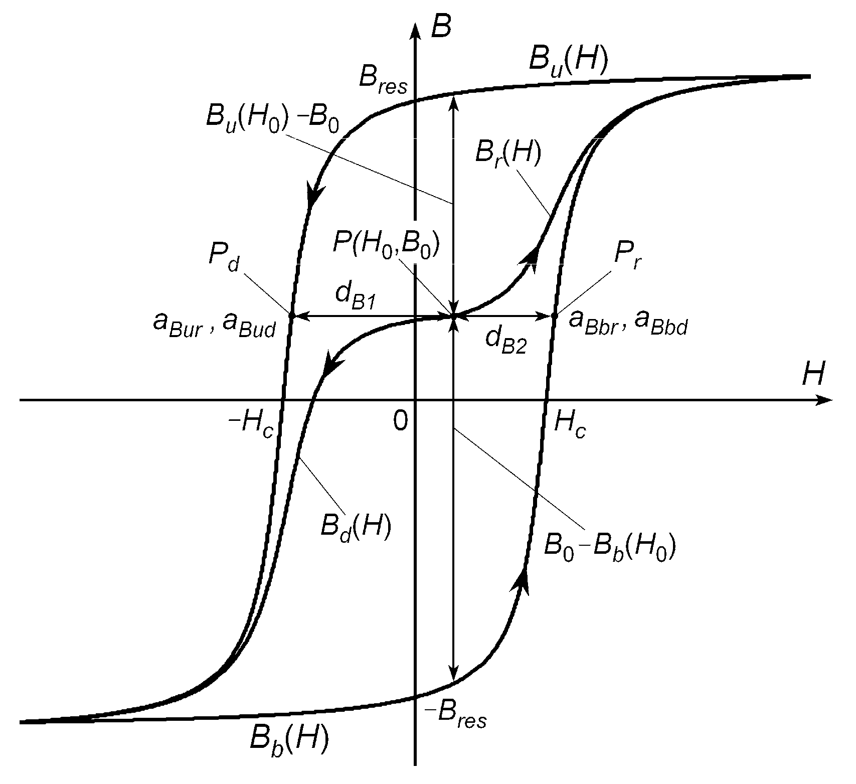
Figure 2.
Dependencies of parameters aBr and aBd on the field strength H0 for B0 = 0: (a) dynamo sheet M530-50A; (b) transformer sheet M120-27S.
Figure 2.
Dependencies of parameters aBr and aBd on the field strength H0 for B0 = 0: (a) dynamo sheet M530-50A; (b) transformer sheet M120-27S.

Figure 3.
Algorithm to determine changes in the flux density.

Figure 4.
Inverse hysteresis loop; dH1 = H0 − Hb(B0), and dH2 = Hu(B0) − H0.

Figure 5.
Dependencies of aHr and aHd on B for H0 = 0 for (a) dynamo sheet M530-50A; (b) transformer sheet M120-27S.
Figure 5.
Dependencies of aHr and aHd on B for H0 = 0 for (a) dynamo sheet M530-50A; (b) transformer sheet M120-27S.

Figure 6.
Algorithm to determine changes in the field strength.

Figure 7.
Family of the first-reversal curves of transformer sheet M120-27S: (a) increasing values of the field strength; (b) decreasing values of the field strength.
Figure 7.
Family of the first-reversal curves of transformer sheet M120-27S: (a) increasing values of the field strength; (b) decreasing values of the field strength.

Figure 8.
Examples of minor loops determined using the approximation: (a) B = f(H); (b) H = f(B).

Figure 9.
Examples of minor loops when the field strength or flux density has a constant component calculated using the approximations (a) B = f(H) and (b) H = f(B).
Figure 9.
Examples of minor loops when the field strength or flux density has a constant component calculated using the approximations (a) B = f(H) and (b) H = f(B).

Figure 10.
Symmetrical hysteresis loops for some assumed values of the field strength: (a) the dynamo sheet M530-50A; (b) the transformer sheet M120-27S for the rolling direction; black line—measured loops, red and blue lines—calculated loops using the basic or inverse approximation of the hysteresis loop.

Figure 11.
Hysteresis loops of transformer sheet M120-27S: (a) for the 45° direction; (b) for the transverse direction; line markings as in Figure 10.
Figure 11.
Hysteresis loops of transformer sheet M120-27S: (a) for the 45° direction; (b) for the transverse direction; line markings as in Figure 10.

Figure 12.
Hysteresis loop of transformer sheet calculated for different values of the exponent: (a) pB; (b) pH; black dashed lines—limiting hysteresis loop, black solid lines—values of the coefficients according to Table 1, red and blue solid lines—values of the coefficients higher or lower 20% according to values in Table 1, respectively.

Figure 13.
Hysteresis loop of (a) Mn-Mg ferrite [50], (b) ferromagnetic material ЮН14ДK24; measured loops—black lines, calculated as B = f(H)—blue lines, calculated as H = f(B)—red lines.
Figure 13.
Hysteresis loop of (a) Mn-Mg ferrite [50], (b) ferromagnetic material ЮН14ДK24; measured loops—black lines, calculated as B = f(H)—blue lines, calculated as H = f(B)—red lines.


Table 1.
Values of parameters pB and pH.
| Electrical Sheet | Angle (Degrees) | Hmax (A/m) | pB | pH | Hmax (A/m) | pB | pH | Hmax (A/m) | pB | pH |
|---|---|---|---|---|---|---|---|---|---|---|
| M530-50A | any | 70 | 3.0 | 0.15 | 105 | 3.0 | 0.20 | 300 | 3.0 | 0.4 |
| M120-27S | 0 | 8 | 2.5 | 0.02 | 12 | 2.5 | 0.025 | 80 | 2.5 | 0.2 |
| M120-27S | 45 | 60 | 1.0 | 0.08 | 100 | 1.0 | 0.10 | 300 | 1.0 | 0.2 |
| M120-27S | 90 | 60 | 2.0 | 0.30 | 100 | 2.0 | 0.40 | 300 | 2.0 | 0.9 |
Publisher’s Note: MDPI stays neutral with regard to jurisdictional claims in published maps and institutional affiliations. |
© 2021 by the authors. Licensee MDPI, Basel, Switzerland. This article is an open access article distributed under the terms and conditions of the Creative Commons Attribution (CC BY) license (https://creativecommons.org/licenses/by/4.0/).
Share and Cite
MDPI and ACS Style
Mazgaj, W.; Sierzega, M.; Szular, Z. Approximation of Hysteresis Changes in Electrical Steel Sheets. Energies 2021, 14, 4110. https://doi.org/10.3390/en14144110
AMA Style
Mazgaj W, Sierzega M, Szular Z. Approximation of Hysteresis Changes in Electrical Steel Sheets. Energies. 2021; 14(14):4110. https://doi.org/10.3390/en14144110
Chicago/Turabian StyleMazgaj, Witold, Michal Sierzega, and Zbigniew Szular. 2021. "Approximation of Hysteresis Changes in Electrical Steel Sheets" Energies 14, no. 14: 4110. https://doi.org/10.3390/en14144110
Note that from the first issue of 2016, this journal uses article numbers instead of page numbers. See further details here.