
The Impact Assessment of Climate Change on Building Energy Consumption in Poland
by
 , ,
, ,
Hassan Bazazzadeh
1,* ,
,
Peiman Pilechiha
2, 
Adam Nadolny
1 ,
,
Mohammadjavad Mahdavinejad
2 and 
Seyedeh sara Hashemi safaei
3 1
Faculty of Architecture, Poznan University of Technology, 61-131 Poznan, Poland
2
Faculty of Architecture, Tarbiat Modares University, Tehran 14115-111, Iran
3
Faculty of Architecture, Jundi-Shapur University of Technology, Dezful 334-64615, Iran
*
Author to whom correspondence should be addressed.
Energies 2021, 14(14), 4084; https://doi.org/10.3390/en14144084
Submission received: 18 May 2021
/
Revised: 26 June 2021
/
Accepted: 28 June 2021
/
Published: 6 July 2021
(This article belongs to the Special Issue Energy Consumption in a Smart City)
Abstract
:A substantial share of the building sector in global energy demand has attracted scholars to focus on the energy efficiency of the building sector. The building’s energy consumption has been projected to increase due to mass urbanization, high living comfort standards, and, more importantly, climate change. While climate change has potential impacts on the rate of energy consumption in buildings, several studies have shown that these impacts differ from one region to another. In response, this paper aimed to investigate the impact of climate change on the heating and cooling energy demands of buildings as influential variables in building energy consumption in the city of Poznan, Poland. In this sense, through the statistical downscaling method and considering the most recent Typical Meteorological Year (2004–2018) as the baseline, the future weather data for 2050 and 2080 of the city of Poznan were produced according to the HadCM3 and A2 GHG scenario. These generated files were then used to simulate the energy demands in 16 building prototypes of the ASHRAE 90.1 standard. The results indicate an average increase in cooling load and a decrease in heating load at 135% and 40%, respectively, by 2080. Due to the higher share of heating load, the total thermal load of the buildings decreased within the study period. Therefore, while the total thermal load is currently under the decrease, to avoid its rise in the future, serious measures should be taken to control the increased cooling demand and, consequently, thermal load and GHG emissions.
1. Introduction
The growth of the urban population due to economic and industrial development has sharply raised the demand for urban infrastructures such as energy systems and housing. These changes, alongside the enhancement of life quality, have led to higher greenhouse gas emissions. Increasing greenhouse gas (GHG) emissions are among the significant causes of climate change, and their impacts include changing weather patterns, extreme weather conditions, and global warming [1]. The Fifth Assessment Report of IPCC (AR5) concluded that as a consequence of these changes, the global mean surface temperature would rise around 2.5–4.5 °C by the end of the 21st century [2]. That is to say, the outdoor climate condition is among the main factors that substantially affect the energy consumption of buildings [3]. This sector, which has a considerably high share in the global energy consumption and total GHG emissions, according to EIA, is a crucial player in the energy context as it accounts for 67% of energy demand worldwide [4] and up to 40% in the E.U. and the U.S. in 2019 [5,6]. Furthermore, it is reported that the total energy-related CO2 emissions of the building sector have risen in recent years after flattening between 2013 and 2016, reaching an all-time high of 10 GtCO2 in 2019 [7]. Therefore, various scholars have tried to address this issue from their own discipline [8].
At the same time, the evidence of climate change indicates its impact on the different aspects of urban life such as health, water resources, energy, economy, and politics. This is why adaptation to climate change is one of the vital challenges of the 21st century to mitigate its adverse effects. Several international committees have attempted to use various methods to study this subject [9]. According to recent studies, the impact of climate change on the building sector can be categorized into “HVAC system”, “heating and cooling demand”, and “power peak demand” [10].
To evaluate the categories above-mentioned, building performance simulation (BPS) helps designers to have a comprehensive energy consumption assessment of a design or an existing building about what it would face during its life cycle. However, studies have indicated that thermal load is a crucial factor in assessing the impact of climate change on a building’s energy consumption as a high proportion of the building’s energy consumption is usually dedicated to heating and cooling systems [11].
To be more precise, the thermal behavior of a building is related to three primary attributes: building physics, the microclimate of the outside environment, and the required thermal comfort inside the building [12]. Therefore, due to the significant impact of weather parameters on building energy demand, an appropriate portion of energy consumption in buildings can be controlled by evaluating only the heating and cooling space demand.
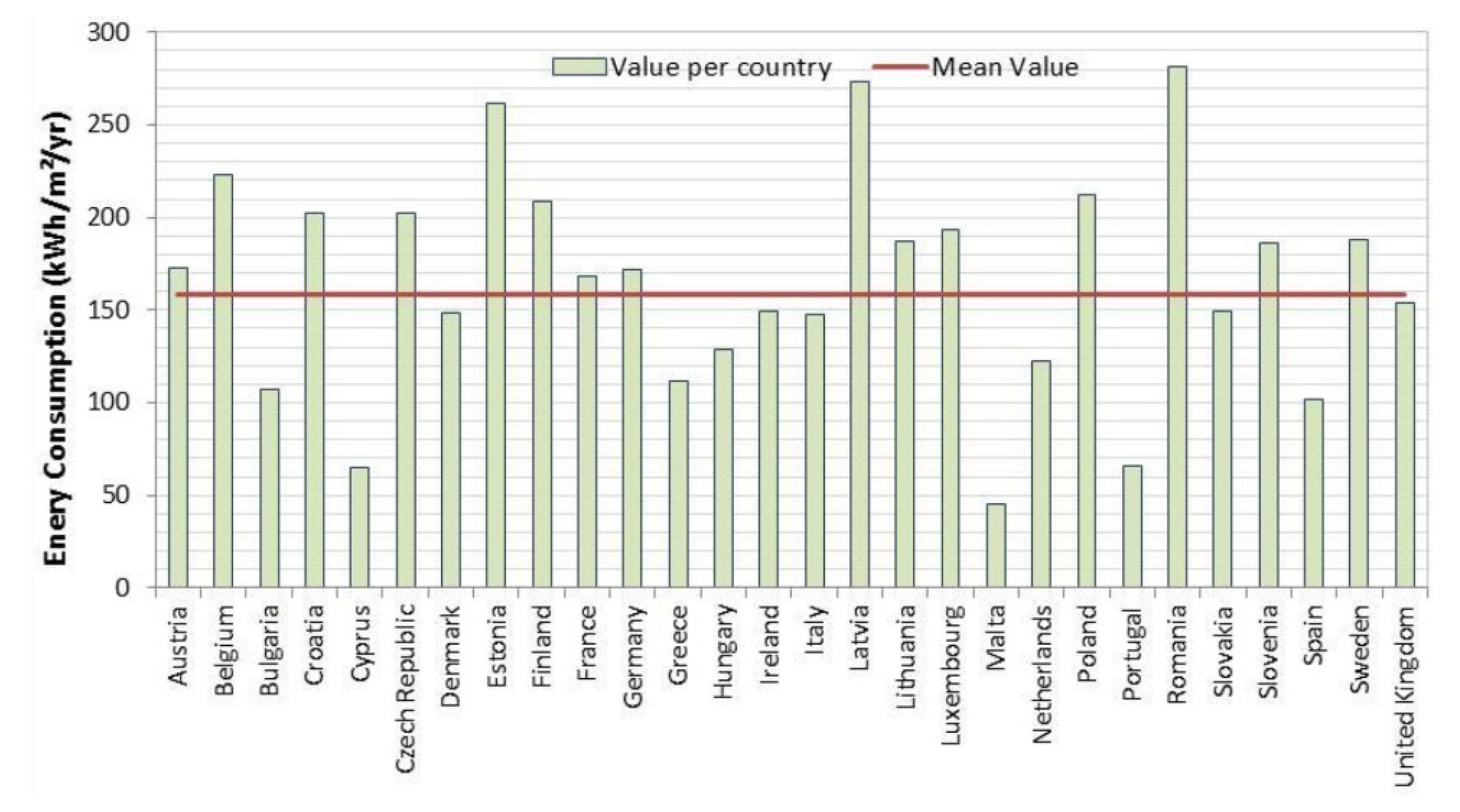
In the E.U., the energy consumption and, more specifically, thermal load in buildings has been decreasing since 2008. In detail, the average annual energy consumption per m2 in the E.U. for all building types in 2013 was around 180 kWh/m2 with different rates for each country (e.g., from 55 kWh/m2 in Malta to 300 kWh/m2 in Romania) according to the illustration of the energy consumption of buildings per m2 (Figure 1). Nevertheless, even for countries with a similar climate, notable differences have been reported (e.g., 200 kWh/m2 in Sweden, 18% lower than Finland). Climatic conditions can mainly explain such discrepancies, which is why there is a crucial need to focus on each country to analyze the impact of climate change on the building’s energy consumption by considering their current and future climatic conditions.
Poland, as one of the top five energy consumers in buildings per m2 in the E.U. (Figure 1) with more than 200 kWh/m2/yr, has experienced substantial growth in energy efficiency by reducing at least 50% of its energy intensity over the last decades [14] thanks to Poland’s Thermo-modernization and Rehabilitation Fund program. However, despite this progress, coal still dominates the power sector. The draft energy policy of Poland has placed a particular emphasis on reducing greenhouse gas (GHG) emissions and increasing the energy efficiency of the building sector. Thus, the Polish government has formed the “Polish National Strategy for Adaptation to Climate Change (NAS 2020)” to focus on an adaptation plan for sectors vulnerable to climate change including the building industry. Among all energy-consuming sectors, the building industry ranked the highest in 2019, with around one-third of total energy consumption. More precisely, residential buildings were responsible for 29% of Poland’s TFC in 2014, and commercial buildings account for roughly 17%. They are also responsible for around 18% of CO2 emissions in Poland since 1990 [15]. The share of the construction sector in Poland’s total energy consumption in recent years is notably high (Figure 2), which indicates the importance of this sector. Furthermore, around three-quarters of Poland’s buildings have either low or deficient energy efficiency standards, according to a survey by “The Buildings Performance Institute Europe (BPIE)” in 2016 [16]. In this sense, climate change can affect Poland’s energy consumption rate, which is why the impact assessment of climate change for the building sector in Poland is quite vital.
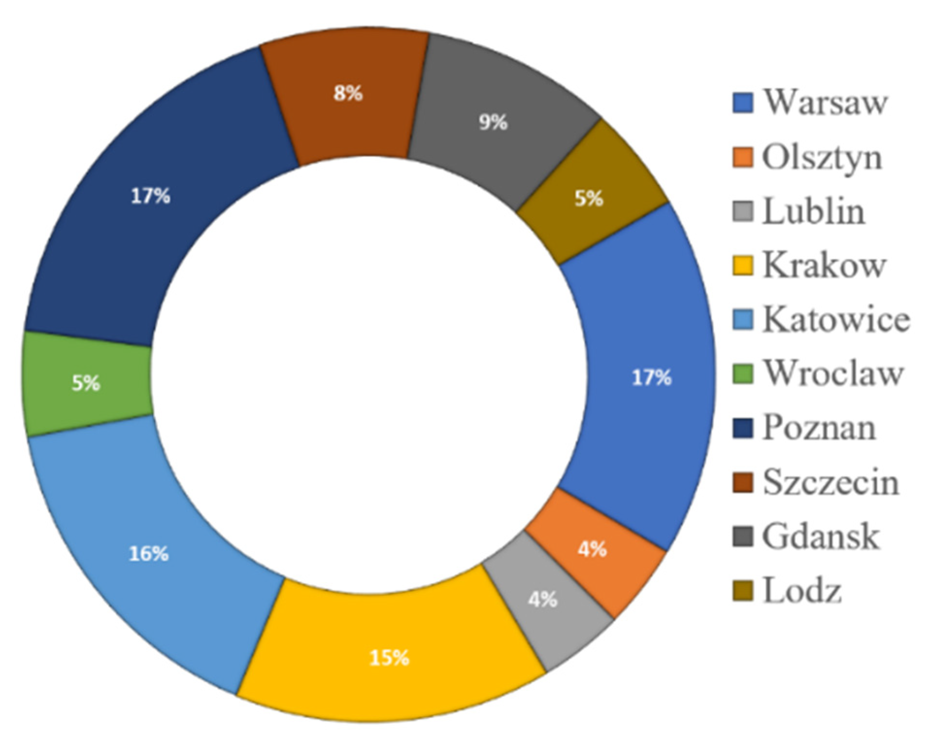
There is an increasing tendency in Poland to enhance energy efficiency, and fortunately, the building sector has always been one of the focal points of this improvement plan. However, limited information and unreliable data about building energy use allow for provisions to circumvent the system [14]. In this respect, solid national cooperation, led by the ‘build desk’, has been formed to address this issue by conducting comprehensive studies to analyze the energy consumption in the building sector in each region. Subsequently, several studies have been carried out in Poznan due to its rapid urban growth and its significance in Poland’s energy sector (Figure 3). Poznan is among the oldest Polish cities in the western region of this country and the fifth-largest city with a population of more than 534,813 according to the 2019 census [18].
In Poznan, in line with the E.U.’s Clean Energy Package goals, an EU-Horizon 2020 project entitled “Energy island communities for energy transition” has started to integrate and demonstrate solutions that will foster a substantial increase in energy efficiency with a total budget of €6,694,000 and one of the energy islands that is going to be studied is “Warta Campus in Poznan” [20]. However, the need for a thorough study of energy performance in different sectors, especially buildings, by considering the current (Cfb according to the Köppen climate classification [20]) and future conditions and uncertainties such as climate change is still crucial (see Table 1). Cfb climate zone, according to the Köppen climate classification, refers to locations where the oceanic climate is temperate; the coldest month averages above 0 °C or − 3 °C, all months had average temperatures below 22 °C, and at least four months averaging above 10 °C. [20]. Therefore, as a response to this need and the significance of the building energy consumption in Poland and, more specifically, in Poznan, this study aimed to analyze the impact of climate change on the thermal load of the building sector in Poznan as a critical node of the E.U. energy-efficient research program.
2. Literature Review
2.1. Projecting Energy Consumption of Buildings
Due to the significance of energy demand, prediction of buildings’ energy demand (more specifically thermal load) has been one of goals of researchers from different perspectives [21,22,23] to reach sustainability [24,25] through optimizing energy consumption [26,27,28]. This knowledge, indeed, can lead to integrated management of buildings [29]. Evaluate and projecting the impact of climate change on building energy consumption and, more specifically, the thermal load, are among the challenging areas for scholars. Rosenthal et al. [30] were among the pioneer scholars who pointed out that the impacts of global warming do not necessarily lead to increased energy expenditure, particularly for reasonably cold regions. They estimated that with 1.0 °C global warming at the end of 2010, the U.S. will save more than $5.5 billion (1991 USD) by reducing energy consumption. Their claim, indeed, is in contrast to earlier studies [31,32] in which an increase in U.S. energy consumption had been projected. In 2006, Nik estimated a sharp decrease in heating load and a more considerable increase of cooling load in Stockholm [33] in 1961–2100 according to uncertainty factors. Christenson and his colleagues [34] reached similar points for Switzerland until 2085. Similarly, Hosseini and her colleagues [35] predicted an average reduction in heating load and an increase in cooling load in Montreal in the period of 2020–2080 by studying a one-storey commercial building.
Cellura [36] studied all scenarios and concluded that we would experience an overall increase in thermal load with a relative decrease in heating and an increase in cooling demand. He stated this by studying 15 cities in southern Europe and generating future weather data by downscaling different general circulation models (GCMs) through the morphing method. To be more precise, he projected that the thermal load of buildings in their study areas increased in a range of 50–119%.
The projections of buildings’ thermal loads influenced by climate change have not always been consistent. That is to say, Crawley [37] concluded that regions with the predominant heating load usually experience a decrease in thermal load. Similarly, Triana, Lamberts, and Sassi asserted that since cooling consumption will significantly increase, the thermal load of social housing will also increase by analyzing the performance of social housing in Sao Paulo and Salvador [38]. Several scholars have reported that this figure could also be increased in a significant number of cases [39,40]. For instance, Shen [41], through the impact assessment of climate change in 2040–2069 for four cities in the U.S. under the IPCC SRES A2 scenario for GHG emissions, reported an average increase and a decrease in annual energy use was reported for residential buildings and office buildings, respectively.
In the most recent studies, Moazami, Nik, and their colleagues [1], by generating several future weather data for Geneva, clarified the importance of considering extreme weather condition for improving the reliability of future weather data. They also indicated that the cooling load would show a more considerable increase (20%) compared to typical conditions. Berardi and Jafarpur [3] also used the statistical downscaling method to analyze the future energy consumption of buildings in Toronto (Dfb zone according to the Köppen—Geiger climate classification [20,42]) by 2070. They discussed that Toronto’s cold climate would see a low magnitude decrease in heating needs and a considerable increase in cooling loads. Additionally, Velashjerdi Farahani et al., to assess the impact of using different passive measures to reduce the risk of overheating in an old and a new apartment in southern Finland, generated future weather data under two scenarios 2050 [43].
2.2. Weather Data
One of the most common kinds of weather data to assess a building’s energy performance and its emission is Typical Meteorological Year (TMY) files. These files consist of 8760 hourly values of selected climatic parameters in which each typical month is selected from different years over a long-term weather dataset [44]. TMY files can be generated through a different method, but the most common method of generating them is using the Finkelstein–Schafer (FS) statistics method, which was developed by Hall et al. [45] and has been widely used by scholars [46]. TMY files are usually generated by considering the data of a long time period as it should represent the typical weather of the intended location. For instance, Petrakis et al., by considering data of seven years, generated TMY for Nicosia in Cyprus [47]. There are also other types of typical meteorological files such as TRY (Typical Reference Year) and DSY (Design Summer Year), which are indeed introduced, analyzed, and modified through various efforts for creating weather data [48,49].
For generating TMY files, according to the definition of these types of weather data, a complete set of historical data is needed to assess before using an acceptable method to choose each month from the years of a dataset. Therefore, the availability of a historical dataset is highly critical. As it is limited for Poznan, which was the case study of this research, the authors, by admitting the fact that different historical weather data may result in some slight differences in the results, used a historical weather dataset of Poznan belonging to 2004–2018, which is relatively recent compared to the usually available TMY files (Table 2).
2.3. Climate Models and Projection
In terms of research method, although GCMs have been widely used for projecting future climate files, they are not quite suitable for building performance simulation purposes as they provide monthly or daily data instead of hourly data needed for BPSs. To consider deviating results of different climate models because of internal climate variability and differences in model formulations, some scholars have used different climate models according to their availability for their study area. For instance, Berardi and Jafarpur, in one of the most recent studies in this area [3], apart from using the HadCM3 model for statistical downscaling, used Hadley Regional Model 3 (HRM3) coupled with Hadley Climate Model 3 (HadCM3) to generate future weather files through dynamical downscaling, which was indeed drawing on their previous work for generating future weather data [50].
More specifically, for climate projection in Poland, the Polish–Norwegian CHASE-PL project helps authors to have a clear overview of Poland’s future climatic conditions influenced by climate change. This projection was obtained through the downscaling of GCM simulations for future conditions. Indeed, model-based projection analyses of CHASEPL were carried out with the ensemble of climate projections comprising nine RCMs outputs stemming from the EURO-CORDEX ensemble for two time periods: 2021–2050 and 2071–2100 [51]. Mezghani et al. illustrated the outcomes of CHASE-PL climate projections [52] and the 5 km (CPLCP-GDPT5) dataset [53]. The projection showed that mean annual temperature is expected to increase by 1 °C until 2021–2050 and by 2 °C until 2071–2100, under the RCP4.5 (an intermediate scenario in which emissions peak around 2040, then decline [54]). However, by considering the RCP8.5 (the worst-case climate change scenario in which emissions continue to rise throughout the 21st century [55]), the same variable was projected to increase to 4 °C by 2071–2100 [56].
Several methods have been widely used to integrate the climate change impacts into weather data according to the current state of this field [57]. These methods can be categorized into two groups: the first group mainly relies on historical weather data and includes the imposed offset method, extrapolating statistical method, and the stochastic weather model. However, the second group relies on numeric climate models instead of historical weather data such as using GCMs to generate local future weather data through downscaling or RCMs. As one of the most widely used methods, downscaling can be performed in two ways: statistical and dynamic downscaling. The dynamic one is a computationally-intensive method that uses the regional scale forcing combined with the lateral boundary condition to generate regional climate models (RCMs) from a GCM.
On the other hand, statistical downscaling is less demanding because its required computations consist of two main stages: the statistical relationship development between large-scale and local climate variables. Second, it uses the previous relationship for the simulation of local climate conditions [58]. By assessing the existing downscaling method, Stephen Belcher introduced a new method of statistical downscaling called “morphing” in 2005 [59]. He discussed dynamic downscaling as being computationally expensive, unlike practical implementation on building design projects. In his study, the stochastic weather generation method that uses empirically derived statistics [60,61] was not considered an efficient way to generate future weather data. Although it is computationally cheap, it requires large datasets to train the model to have a reliable model, and the weather series it produces may not always be meteorologically consistent.
Although several scholars such as Nik [33] are still employing other methods such as regional climate models (RCMs) to downscale the results of the GCMs dynamically, they mainly need special requirements for the generated data. For instance, Nik’s work better represented topography and mesoscale processes than the statistical downscaling employed by authors to use other methods rather than morphing. However, in general, statistical downscaling and, more specifically, morphing has recently been one of the main preferred methods chosen by scholars for its relatively low computational requirements and fast calculations [3,62,63,64,65,66,67].
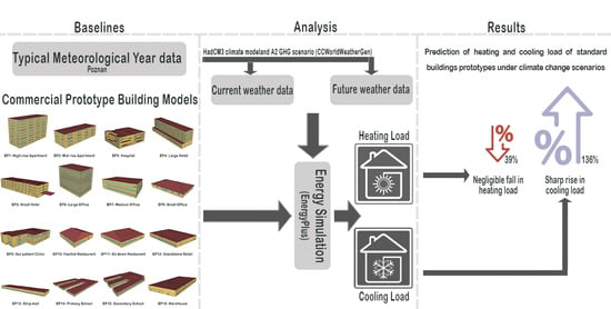
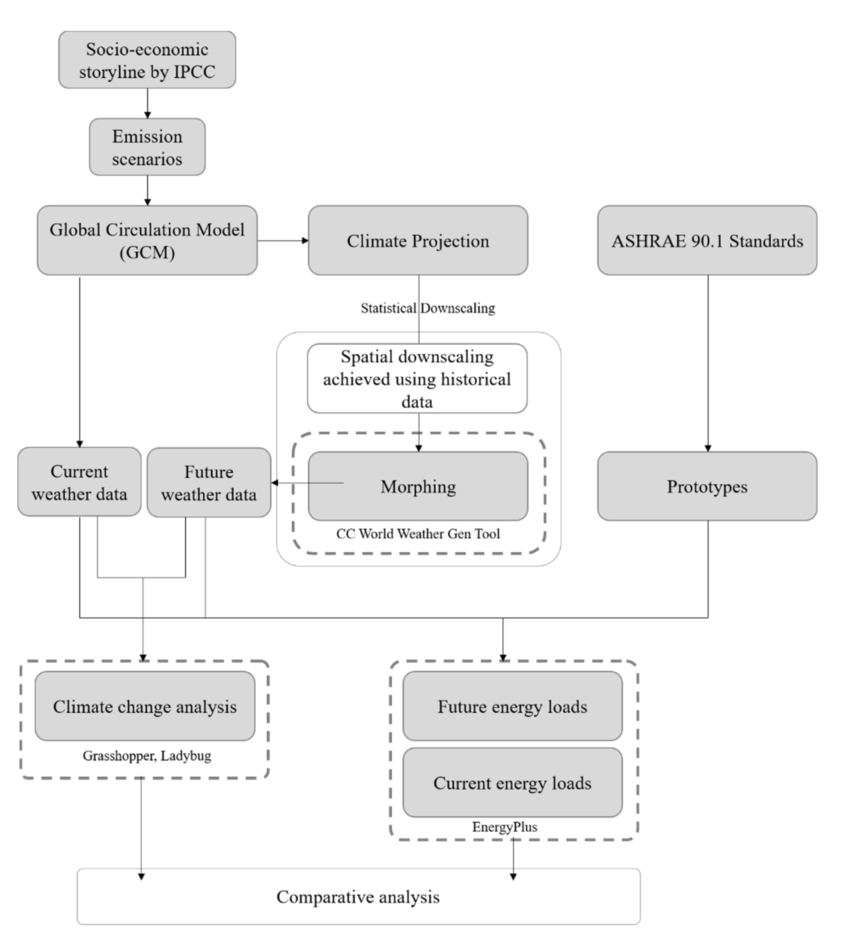
3. Methodology
For the research case study, a set of historical data in the form of a Typical Meteorological Year (TMY file) was used as it was very recent compared to the typical TMY files available for most locations in Poland. In this research, as the first step, a weather file from the Ławica Airport weather station in Poznan was used as the baseline of projection.
These data were obtained from GCMs, and subsequently used as an input in the Climate Change World Weather Generator (CCWorldWeatherGen; the Sustainable energy research group (SERG) at Southampton university, Southampton, England) tool for projection. Initially developed by Jentsch [68,69], the Microsoft® Excel-based tool called the ‘Climate Change World Weather Generator’, commonly referred to as CCWorldWeatherGen, uses the output data of HadCM3 (Met Office Hadley Centre for Climate Science and Services; 2010), forced with the IPCC A2 emission scenario to generate future weather files by applying the morphing method. Jentsch et al., after assessing 23 GCMs under AR4 and six GCMs under AR3 around the world, showed that HadCM3 for the A2 emission scenario seems like a suitable GCM for use in the morphing technique [69]. This emission scenario put forward by the IPCC AR3 refers to a ‘business as usual’ condition in which the global population would continuously increase, and regionally oriented economic growth would grow. Therefore, it is evident that using HadCM3 for the A2 emission scenario for this tool, which uses a morphing method, is appropriate. Thus, this tool helps scholars have a fast projection about the future of climate change [70]. In detail, by adding the TMY file into CCWorldWeatherGen, the future weather data for 2050 and 2080 were created under the A2 scenario through the morphing procedure. The data obtained from GCMs were subsequently used as an input in CCWorldWeatherGen to statistically downscale the baseline and generate future weather data in the second stage. In this research, the life cycles of buildings were assumed to be at least 60 years, which means that up to the end of the analysis period, there would be no changes in the performance of building components in terms of thermal load.
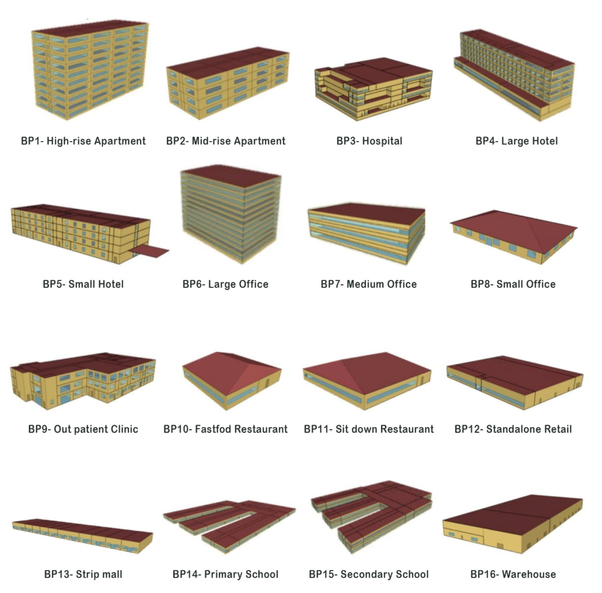
Finally, current and future weather files were used to perform building energy modeling using EnergyPlus 9.0.1. To simulate the impact of climate change on the buildings’ thermal load for the city of Poznan, 16 building prototypes of the ASHRAE standard 90.1 were chosen to be used in this study [71] to assess the impact of climate change on a building’s thermal load. These prototypes were initially obtained from DOE’s Commercial Reference Building Models with modifications from the Advanced Energy Design Guide series and the ASHRAE 90.1 committee. Their detailed descriptions and modeling strategies are accessible in the Pacific Northwest National Laboratory’s (PNNL) reports [72,73]. Having realistic building characteristics, these 16 prototypes (Figure 4) were simulated with the current and future weather data to compare the relative impact of climate change on their energy performance. Technical descriptions of the prototypes’ envelope components are presented as given in Table 3.
After performing the energy simulation for each prototype using current and future climate weather files, the comparative analysis showed the impact of climate change on the thermal load of buildings, which was the primary goal of this paper (Figure 5).
4. Results
This section initially presents the results of the weather projection and the comparison between projected values and the current conditions to provide an overview of the future trend of climatic condition in Poznan. This section is followed by employing each weather data to build a prototype to assess the impact of climate change on their thermal load.
Comparing current and generated future weather data for the next 30 and 60 years showed the future trend discussed in detail. There were 13 influential variables that this study took into account, namely: dry bulb temperature, dew point temperature, relative humidity, direct normal radiation, global horizontal radiation, diffuse horizontal radiation, horizontal infrared radiation, direct normal illuminance, global horizontal illuminance, diffuse horizontal illuminance, ground temperature, total sky cover, and atmospheric pressure.
The future weather files forecast a notably warmer period with more direct illuminance and radiation and less humidity with lower clouds in the sky (Table 4). In general, the temperature-related variables showed an average increase of 4 °C in this period, while this figure for the radiation and illuminances group was around 14.3 Wh/m2 and 463 lux, respectively. On the other hand, although the change rate for total sky cover was considerable with an almost 15% decrease, rates for atmospheric pressure were negligible. To be more precise, the highest increase belonged to direct normal illuminance at around one third, while the figure for atmospheric pressure ranked last. In contrast, total sky cover had the highest decrease (−13%), and the lowest decrease belonged to diffuse horizontal illuminance less than 1%.
The next step to assess the impact of climate change on the building’s energy consumption, heating and cooling use intensity (EUI), and thermal load for all 16 prototypes were calculated, and the results are as follows. After the simulation process, the values for heating and cooling EUI were mapped in scatterplot graphs, and trendlines of these variables for each prototype were drawn. As expected, the heating load for most cases saw a steady fall while the cooling load showed a sharp rise in the study period.
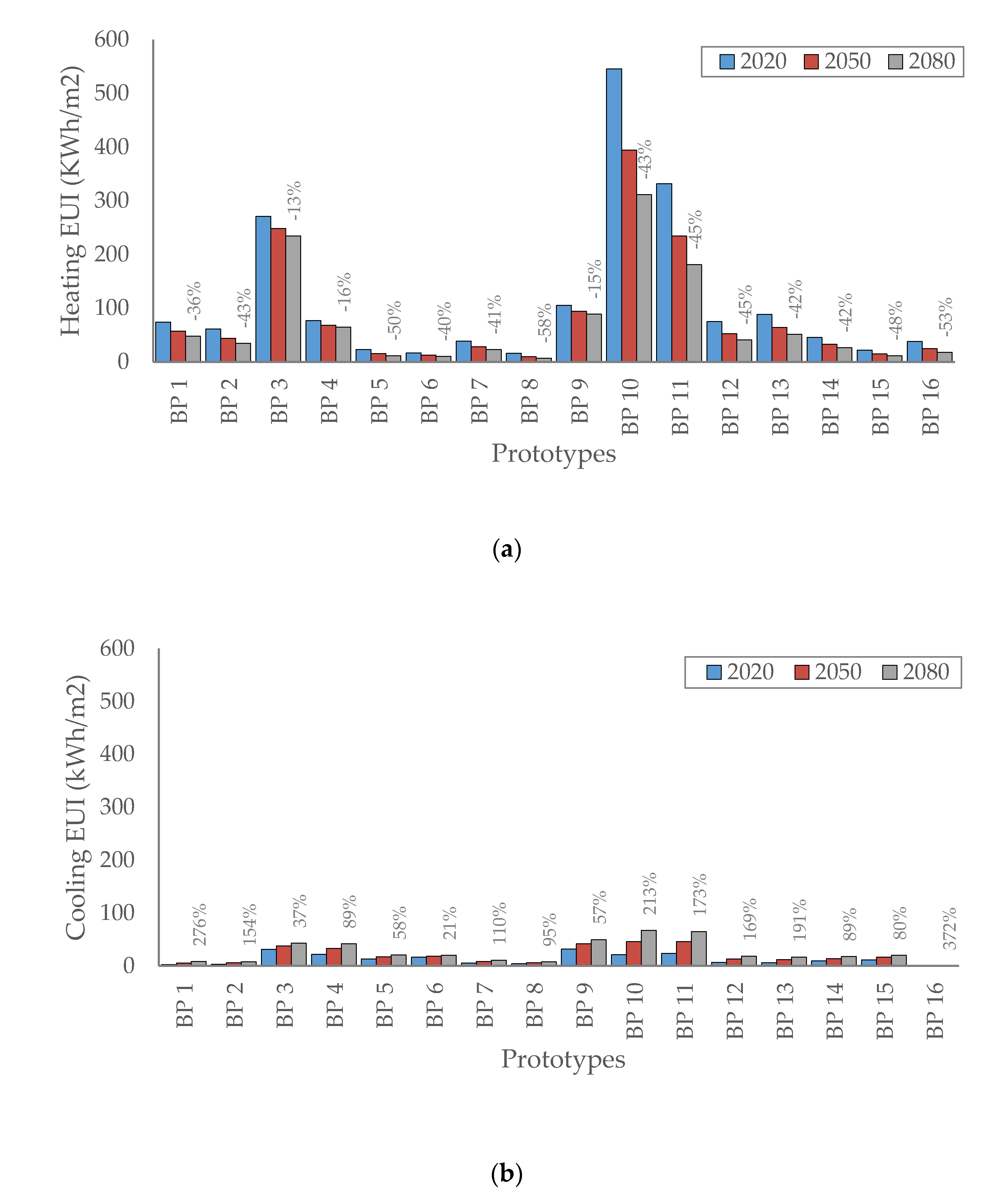
In terms of heating EUI, a blatant downward trend with different decrease rates, depending on building prototypes with an average decrease of more than 41 kWh/m2, was witnessed (Figure 6a). The heating load average value in 2020 was around 114 kWh/m2, while for 2050 and 2080, it was more than 87 kWh/m2 and 72 kWh/m2 with a roughly 25% and 40% decrease, respectively. To be more specific, the heating load of the fast-food restaurant building (BP10) significantly decreased (324 kWh/m2) while in contrast, in the large office building (BP06), the decrease was not considerable (around 6 kWh/m2). On the other hand, while heating load changed averagely near 40% in building prototypes, the maximum decrease belonged to the small office building (BP08) with around 57%, and the minimum was for the hospital building (BP03) at roughly 13%.
As far as the cooling load is concerned, the results indicated a clear, stable upward trend in the cooling load with an average increase of 13 kWh/m2 (Figure 6b). Indeed, while the average cooling load in 2020 was 13 kWh/m2, it increased 1.5 and 2 times in 2050 and 2080, respectively. Among all BPS, the cooling load of the fast-food restaurant building (BP10) increased markedly (46 kWh/m2) while the warehouse building (BP16) increased slightly (0.7 kWh/m2). All prototypes saw the average increase rate of cooling load at 135%, while the maximum increase rate belonged to the warehouse building (BP16) with 371% and the minimum one was for the large office building (BP06) with 20%.
Comparing the heating and cooling from 2020 to 2080, a considerable difference was noticeable. The results suggest that increasing the cooling load was certain, and the heating load decreased for all cases. It is evident that although the average rate absolute change for the cooling load was 13 kWh/m2, which was notably lower than that of the heating load with more than 41 kWh/m2, the percentages of this change were roughly 135% and 40%, respectively. This difference indicates the relatively sharp rise of the cooling load and negligible decrease in heating load for Poznan in the study period. The highest relative difference change rate of the heating load was witnessed in the small office (BP08) with around a 60% (around 10 kWh/m2) decrease. In addition, the relative change rate of the cooling load was reported to be the highest in the warehouse building (BP16) at 372%, where the absolute figure of this change was the lowest (0.7 kWh/m2).
On the other hand, the lowest relative change rate of the heating and cooling load was for the hospital (BP03) with a 13% decrease and the large office building (BP06) with a 58% increase. Due to global warming, which has already started, the need for cooling has increased relatively higher. Therefore, the demand for heating energy would decrease. Indeed, according to this figure, the role of cooling load, which is not as important as heating load due to its small share in the thermal load within the study period, would probably be more significant as this share is changing.
5. Discussion
Required data availability and quality are essential for successful scenario projections, especially to assess the built environment where accurate energy data are very critical [75]. Admittedly, using a different historical weather dataset for different periods could provide an overview of the accuracy of the results by comparing their outcomes. However, the unavailability of historic weather datasets is among the limitations of studies, which is why only one set of historical weather data was used in this study. Moreover, in contrast to megacities, there are various climate projections according to different climate models; Poznan’s only available climate model for projection was the HadCM3 and IPCC A2 emission scenario.
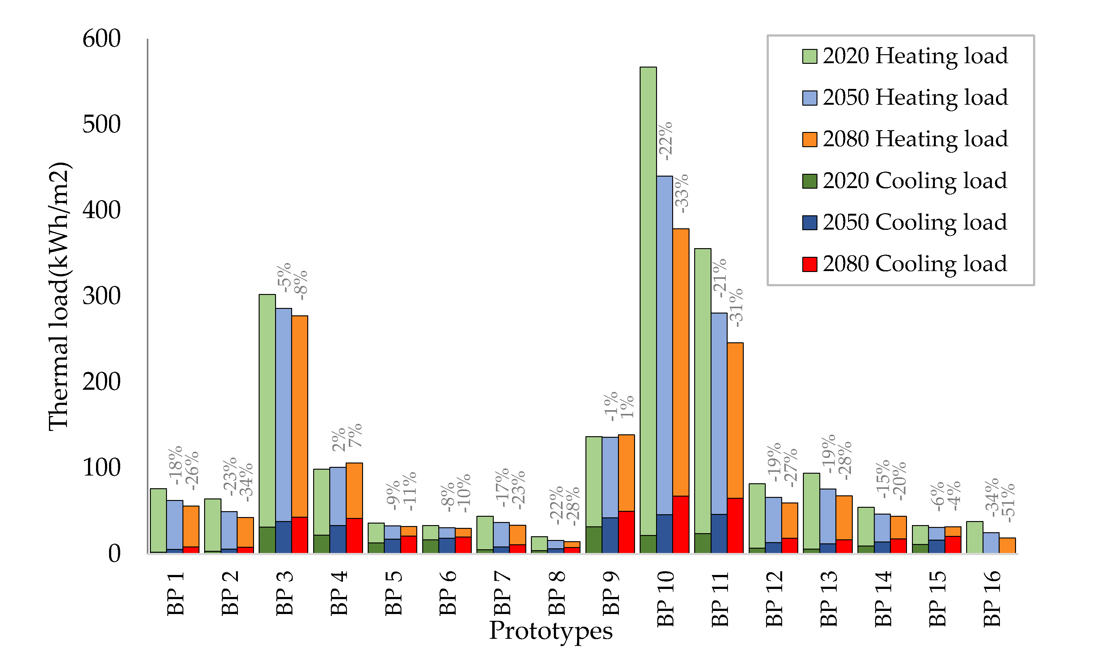
It should be noted that solely comparing the relative changing rate of heating and cooling demand cannot give us a clear image of the thermal load’s future as the initial magnitude of these figures was highly distinguished. In other words, although the relative changing rate of cooling demand was about three times higher than that of the heating load, however, as the share of cooling load in 2020 was considered negligible, this change would not change the pattern of total thermal load extensively. As shown in Figure 7, most BPs showed a relatively downward trend with different rates, with an average decrease of roughly 28 kWh/m2 in thermal loads. To be more specific, while the average rate of changing thermal load was 20% (decrease), the minimum value was observed in the outpatient health care building (BP09) with 1% positive change, and the maximum value was for the warehouse building (BP16) with more than 50% negative change. Therefore, it can be concluded that the decrease rate in thermal loads in most cases was slight. The decrease rate also shows that despite the increasing trend of cooling load, its contribution in thermal load was negligible such as in the large hotel building (BP04) and the outpatient health care building (BP09) where the drop in the heating load was not sharp like in other cases, where the thermal load increased. The results predicted that while the average thermal load of cases was around 127 kWh/m2, this figure changed for 2080 at around 98 kWh/m2 with a more than 22% decrease. It was also reported that the slightest decrease in thermal load associated with the secondary school building (BP15) with 1.3 kWh/m2, and the maximum value was for the fast-food restaurant building (BP10) with 188 kWh/m2.
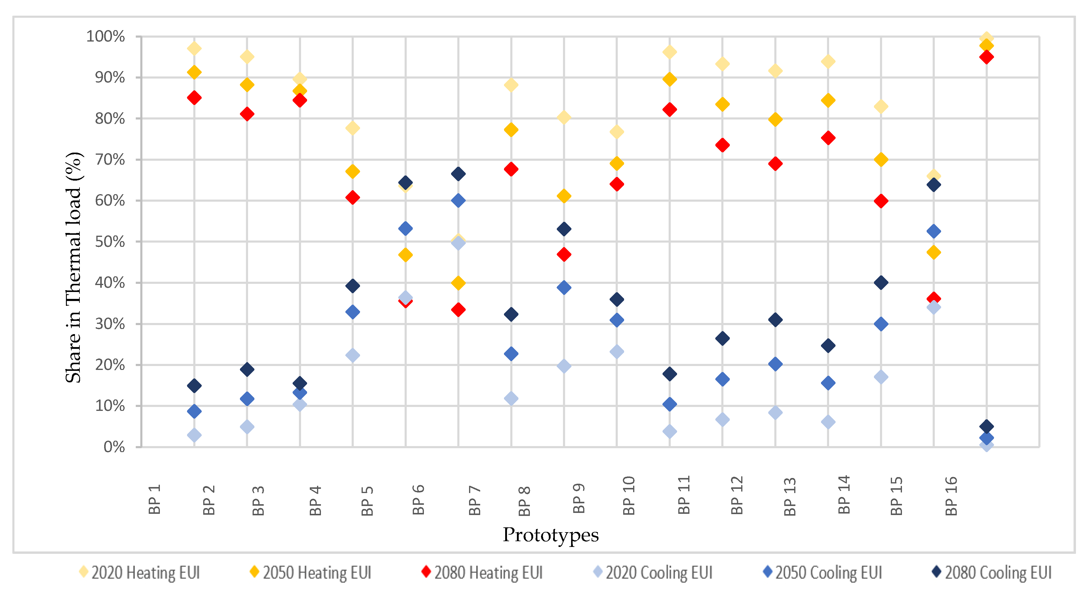
Despite the upward trend in the cooling loads, their contributions in thermal load were still lower than heating loads in most BPs. In a more detailed report (Figure 8), in 25% of prototypes (BP05, BP06, BP08, and BP15), the contribution of cooling and heating load in 2080 was reversed in another group with the same size (BP01, BP02, BP03, and BP16). Therefore, a considerable difference between the contribution of heating and cooling load has remained. Therefore, it can be concluded that the closer the heating and cooling contributions were, the more likely the contributions were to reverse.
Therefore, considering the earlier discussions, it can be concluded that, in general, climate change heavily changed the energy performance of all building prototypes through increasing cooling and decreasing heating load. In this sense, as the contribution of cooling was more petite than heating in most cases, the total thermal load of most cases was reduced due to the decreased heating load. Furthermore, in one quarter of cases, the cooling increment altered heating and cooling contributions in thermal load. Finally, whenever increased heating load was reported, the total thermal load showed an upward trend in the study period.
6. Conclusions
These days, we are witnessing that the share of the building sector in the total world energy consumption has been reported to be critically high, and it has also been predicted to increase for several reasons. These changes may lead to higher GHG emissions, one of the significant reasons behind climate change that can potentially affect the buildings’ thermal load. As the impacts of climate change on a building’s energy consumption have been different from one region to another according to several studies, this paper presents the impact assessment of climate change on the energy performance buildings for Poznan city in Poland. Furthermore, the current state literature established the importance of considering future weather data to evaluate the buildings’ energy performance. This is why generating future weather data based on statistical downscaling in the initial part of this paper enabled the authors to project the energy demand of prototypes in the future. Thus, one of the prevailing methods for generating future weather data, using the HadCM3 climate model and considering IPCC SRES A2 GHG scenario through statistical downscaling future weather data for Poznan for 2020–2080, was generated.
According to the developed future weather data, Poznan will see a notable increase in average temperature in the following 60 years. In this sense, changing the climate zone of Poznan would be a strong possibility. The results indicated that the cooling load of prototypes was in the mid-range, which is why the despite the negligible rate of cooling load in total thermal load compared to the share of heating load, almost all prototypes saw a sharp rise in cooling load and a slight fall in heating load at around 135% and 40% by 2080, respectively. This change led to altering the most significant share in total thermal load from heating load to cooling load in 25% of prototypes, but for other cases where heating load remained the highest share, the total thermal loads saw a steady decrease in the study period. Similar to other studies in this area, in general, it can be concluded that as the average temperature of Poznan will rise from 2020 to 2080, the climate zone of this region will probably shift as other scholars have had such predictions for cities with similar climatical conditions. As a result, the heating demand will decrease, and the cooling demand will substantially increase. However, what has been missing in the studies is the impact on the total thermal load. According to the results, the total thermal load of more than 85% of prototypes decreased because of the sharp decrease in heating loads. Therefore, by comparing the change rate of total thermal load and heating load, it is evident that the more heating load a prototype consumes, the more likely it will see a decrease in total thermal load in the future. It should also be noted that considering only the HadCM3 climate model for the A2 emission scenario was one of the limitations of this research.
The impacts of predicted climate change were seen in mild cooling seasons and warmer heating seasons. Buildings with high heating loads will likely decrease the total thermal load for the next 60 years for a cold Polish climate. Therefore, buildings that tend to sustain for decades should evaluate how their cooling load can be reduced as increasing it will lead to more GHG emissions and more extreme weather conditions. This evaluation means that to mitigate the impact of climate change on the energy load of buildings, it is highly critical to investigate ways to understand the energy resiliency of buildings. Future studies should consider a broader range of scenarios and use other climate models to increase the study’s accuracy. Furthermore, conducting a comprehensive study about all major cities of Poland would be a real boon for Polish decision-makers.
Author Contributions
Conceptualization, H.B., P.P., A.N., and M.M.; Methodology, H.B., P.P., and S.H.; Software, H.B. and S.H.; Validation, H.B., P.P., and M.M.; Formal analysis, H.B., P.P., and S.H.; Investigation, H.B.; Resources, H.B. and S.H.; Data curation, H.B. and S.H.; Writing—original draft preparation, H.B. and S.H.; Writing—review and editing, P.P., A.N., and M.M.; Visualization, H.B. and S.H.; Supervision, P.P., A.N., and M.M.; Project administration, H.B. and A.N.; Funding acquisition, H.B. and A.N. All authors have read and agreed to the published version of the manuscript.
Funding
This research was funded by Poznan University of Technology, within the framework of the research project entitled “Mapping of architectural space, the history, theory, practice, contemporaneity II”, grant number 0112/SBAD/0185.
Institutional Review Board Statement
Not applicable.
Informed Consent Statement
Not applicable.
Data Availability Statement
Not applicable.
Conflicts of Interest
The authors declare no conflict of interest.
References
- Moazami, A.; Nik, V.M.; Carlucci, S.; Geving, S. Impacts of future weather data typology on building energy performance—Investigating long-term patterns of climate change and extreme weather conditions. Appl. Energy 2019, 238, 696–720. [Google Scholar] [CrossRef]
- IPCC. Synthesis Report Contribution of Working Groups I, II and III to the Fifth Assessment Report of the Intergovernmental Panel on Climate Change; IPCC: Geneva, Switzerland, 2014. [Google Scholar]
- Berardi, U.; Jafarpur, P. Assessing the impact of climate change on building heating and cooling energy demand in Canada. Renew. Sustain. Energy Rev. 2020, 121, 109681. [Google Scholar] [CrossRef]
- Madlener, R.; Sunak, Y. Impacts of urbanization on urban structures and energy demand: What can we learn for urban energy planning and urbanization management? Sustain. Cities Soc. 2011, 1, 45–53. [Google Scholar] [CrossRef]
- Cao, X.; Dai, X.; Liu, J. Building energy-consumption status worldwide and the state-of-the-art technologies for zero-energy buildings during the past decade. Energy Build. 2016, 128, 198–213. [Google Scholar] [CrossRef]
- Bazazzadeh, H.; Nadolny, A.; Hashemi Safaei, S.S. Climate Change and Building Energy Consumption: A Review of the Impact of Weather Parameters Influenced by Climate Change on Household Heating and Cooling Demands of Buildings. Eur. J. Sustain. Dev. 2021, 10, 1. [Google Scholar] [CrossRef]
- IEA. Tracking Buildings 2020; IEA: Paris, France, 2020. [Google Scholar]
- Tabrizikahou, A.; Nowotarski, P. Mitigating the Energy Consumption and the Carbon Emission in the Building Structures by Optimization of the Construction Processes. Energies 2021, 14, 3287. [Google Scholar] [CrossRef]
- Mancini, F.; Lo Basso, G. How Climate Change Affects the Building Energy Consumptions Due to Cooling, Heating, and Electricity Demands of Italian Residential Sector. Energies 2020, 13, 410. [Google Scholar] [CrossRef] [Green Version]
- Yau, Y.H.; Hasbi, S. A review of climate change impacts on commercial buildings and their technical services in the tropics. Renew. Sustain. Energy Rev. 2013, 18, 430–441. [Google Scholar] [CrossRef]
- Kheiri, F. A review on optimization methods applied in energy-efficient building geometry and envelope design. Renew. Sustain. Energy Rev. 2018, 92, 897–920. [Google Scholar] [CrossRef]
- Gero, J.S.; D’Cruz, N.; Radford, A.D. Energy in context: A multicriteria model for building design. Build. Environ. 1983, 18, 99–107. [Google Scholar] [CrossRef]
- European Commission (EC). Energy Consumption of Buildings per m²; European Commission, 2013. Available online: https://ec.europa.eu/energy/content/energy-consumption-m%C2%B2-2_en (accessed on 30 May 2021).
- Stuggins, G.; Sharabaroff, A.; Semikolenova, Y. Energy Efficiency; Lessons Learned from Success Stories; The World Bank: Washington, DC, USA, 2013. [Google Scholar] [CrossRef]
- IEA. Energy Policies of IEA Countries: Poland 2016 Review; IEA: Paris, France, 2017. [Google Scholar]
- Staniaszek, D.; Firląg, S. Financing Building Energy Performance Improvement in Poland; BPIE: Brussels, Belgium, 2016. [Google Scholar]
- BuildDeskPolska. Energy Condition of Buildings in Poland; BuildDeskPolska: Cigacice, Poland, 2011. [Google Scholar]
- Parysek, J.J.; Mierzejewska, L. Poznań. Cities 2006, 23, 291–305. [Google Scholar] [CrossRef]
- BuildDeskPolska. BuildDesk Analytics Report; Energy Condition of Buildings in Poland; BuildDeskPolska: Cigacice, Poland, 2019. [Google Scholar]
- European Union (EU). Energy Island Communities for Energy Transition. Available online: https://cordis.europa.eu/project/id/957845/pl (accessed on 17 February 2021).
- Seyedzadeh, S.; Pour Rahimian, F.; Oliver, S.; Rodriguez, S.; Glesk, I. Machine learning modelling for predicting non-domestic buildings energy performance: A model to support deep energy retrofit decision-making. Appl. Energy 2020, 279, 115908. [Google Scholar] [CrossRef]
- Eslamirad, N.; Malekpour Kolbadinejad, S.; Mahdavinejad, M.; Mehranrad, M. Thermal comfort prediction by applying supervised machine learning in green sidewalks of Tehran. Smart Sustain. Built Environ. 2020, 9, 361–374. [Google Scholar] [CrossRef]
- Ghaffour, W.; Ouissi, M.N.; Velay Dabat, M.A. Analysis of urban thermal environments based on the perception and simulation of the microclimate in the historic city of Tlemcen. Smart Sustain. Built Environ. 2021, 10, 141–168. [Google Scholar] [CrossRef]
- Thanu, H.P.; Rajasekaran, C.; Deepak, M.D. Developing a building performance score model for assessing the sustainability of buildings. Smart Sustain. Built Environ. 2020. ahead-of-print. [Google Scholar] [CrossRef]
- Rahmouni, S.; Smail, R. A design approach towards sustainable buildings in Algeria. Smart Sustain. Built Environ. 2020, 9, 229–245. [Google Scholar] [CrossRef]
- Dell’Anna, F.; Bottero, M.; Becchio, C.; Corgnati, S.P.; Mondini, G. Designing a decision support system to evaluate the environmental and extra-economic performances of a nearly zero-energy building. Smart Sustain. Built Environ. 2020, 9, 413–442. [Google Scholar] [CrossRef]
- Seyedzadeh, S.; Pour Rahimian, F. Building Energy Data-Driven Model Improved by Multi-objective Optimisation. In Data-Driven Modelling of Non-Domestic Buildings Energy Performance: Supporting Building Retrofit Planning; Seyedzadeh, S., Pour Rahimian, F., Eds.; Springer International Publishing: Cham, The Netherlands, 2021; pp. 99–109. [Google Scholar] [CrossRef]
- Weiss, T. Energy flexibility and shiftable heating power of building components and technologies. Smart Sustain. Built Environ. 2020. ahead-of-print. [Google Scholar] [CrossRef]
- Sheikhkhoshkar, M.; Pour Rahimian, F.; Kaveh, M.H.; Hosseini, M.R.; Edwards, D.J. Automated planning of concrete joint layouts with 4D-BIM. Autom. Constr. 2019, 107, 102943. [Google Scholar] [CrossRef]
- Kottek, M.; Grieser, J.; Beck, C.; Rudolf, B.; Rubel, F. World Map of the Köppen-Geiger climate classification updated. Meteorol. Z. 2006, 15, 5. [Google Scholar] [CrossRef]
- Rosenthal, D.H.; Gruenspecht, H.K.; Moran, E.A. Effects of Global Warming on Energy Use for Space Heating and Cooling in the United States. Energy J. 1995, 16, 77–96. [Google Scholar] [CrossRef]
- Nordhaus, W.D. To slow or not to slow: The economics of the greenhouse effect. Econ. J. 1991, 101, 17. [Google Scholar] [CrossRef]
- Cline, W.R. The Economics of Global Warming; Institute for International Economics: Washington, DC, USA, 1992. [Google Scholar]
- Nik, V.M.; Sasic Kalagasidis, A. Impact study of the climate change on the energy performance of the building stock in Stockholm considering four climate uncertainties. Build. Environ. 2013, 60, 291–304. [Google Scholar] [CrossRef]
- Christenson, M.; Manz, H.; Gyalistras, D. Climate warming impact on degree-days and building energy demand in Switzerland. Energy Convers. Manag. 2006, 47, 671–686. [Google Scholar] [CrossRef]
- Hosseini, M.; Tardy, F.; Lee, B. Cooling and heating energy performance of a building with a variety of roof designs; the effects of future weather data in a cold climate. J. Build. Eng. 2018, 17, 107–114. [Google Scholar] [CrossRef] [Green Version]
- Cellura, M.; Guarino, F.; Longo, S.; Tumminia, G. Climate change and the building sector: Modelling and energy implications to an office building in southern Europe. Energy Sustain. Dev. 2018, 45, 46–65. [Google Scholar] [CrossRef]
- Crawley, D.B. Estimating the impacts of climate change and urbanization on building performance. J. Build. Perform. Simul. 2008, 1, 91–115. [Google Scholar] [CrossRef]
- Triana, M.A.; Lamberts, R.; Sassi, P. Should we consider climate change for Brazilian social housing? Assessment of energy efficiency adaptation measures. Energy Build. 2018, 158, 1379–1392. [Google Scholar] [CrossRef] [Green Version]
- Wang, H.; Chen, Q. Impact of climate change heating and cooling energy use in buildings in the United States. Energy Build. 2014, 82, 428–436. [Google Scholar] [CrossRef] [Green Version]
- Cox, R.A.; Drews, M.; Rode, C.; Nielsen, S.B. Simple future weather files for estimating heating and cooling demand. Build. Environ. 2015, 83, 104–114. [Google Scholar] [CrossRef] [Green Version]
- Shen, P. Impacts of climate change on U.S. building energy use by using downscaled hourly future weather data. Energy Build. 2017, 134, 61–70. [Google Scholar] [CrossRef]
- Rubel, F.; Brugger, K.; Klaus, H.; Auer, I. The climate of the European Alps: Shift of very high resolution Köppen-Geiger climate zones 1800–2100. Meteorol. Z. 2017, 26, 11. [Google Scholar] [CrossRef]
- Velashjerdi Farahani, A.; Jokisalo, J.; Korhonen, N.; Jylhä, K.; Ruosteenoja, K.; Kosonen, R. Overheating Risk and Energy Demand of Nordic Old and New Apartment Buildings during Average and Extreme Weather Conditions under a Changing Climate. Appl. Sci. 2021, 11, 3972. [Google Scholar] [CrossRef]
- Herrera, M.; Natarajan, S.; Coley, D.A.; Kershaw, T.; Ramallo-González, A.P.; Eames, M.; Fosas, D.; Wood, M. A review of current and future weather data for building simulation. Build. Serv. Eng. Res. Technol. 2017, 38, 602–627. [Google Scholar] [CrossRef] [Green Version]
- Hall, I.J.; Prairie, R.R.; Anderson, H.E.; Boes, E.C. Generation of a typical meteorological year. In Proceedings of the 1978 Annual Meeting of American Section of ISES, Denver, CO, USA, 12–15 August 1978. [Google Scholar]
- Lam, J.C.; Hui, S.C.M.; Chan, A.L.S. A Statistical Approach to the Development of a Typical Meteorological Year for Hong Kong. Archit. Sci. Rev. 1996, 39, 201–209. [Google Scholar] [CrossRef]
- Petrakis, M.; Kambezidis, H.D.; Lykoudis, S.; Adamopoulos, A.D.; Kassomenos, P.; Michaelides, I.M.; Kalogirou, S.A.; Roditis, G.; Chrysis, I.; Hadjigianni, A. Generation of a “typical meteorological year” for Nicosia, Cyprus. Renew. Energy 1998, 13, 381–388. [Google Scholar] [CrossRef]
- Bilbao, J.; Miguel, A.; Franco, J.; Ayuso, A. Test Reference Year Generation and Evaluation Methods in the Continental Mediterranean Area. J. Appl. Meteorol. 2004, 43, 390–400. [Google Scholar] [CrossRef]
- Chan, A.L.S.; Chow, T.T.; Fong, S.K.F.; Lin, J.Z. Generation of a typical meteorological year for Hong Kong. Energy Convers. Manag. 2006, 47, 87–96. [Google Scholar] [CrossRef]
- Jafarpur, P.; Berardi, U. Building energy demand within a climate change perspective. IOP Conf. Series Mater. Sci. Eng. 2019, 609, 072037. [Google Scholar] [CrossRef]
- Kundzewicz, Z.W.; Piniewski, M.; Mezghani, A.; Okruszko, T.; Pińskwar, I.; Kardel, I.; Hov, Ø.; Szcześniak, M.; Szwed, M.; Benestad, R.E.; et al. Assessment of climate change and associated impact on selected sectors in Poland. Acta Geophys. 2018, 66, 1509–1523. [Google Scholar] [CrossRef] [Green Version]
- Mezghani, A.; Dobler, A.; Haugen, J.E.; Benestad, R.E.; Parding, K.M.; Piniewski, M.; Kardel, I.; Kundzewicz, Z.W. CHASE-PL Climate Projection dataset over Poland—Bias adjustment of EURO-CORDEX simulations. Earth Syst. Sci. Data 2017, 9, 905–925. [Google Scholar] [CrossRef] [Green Version]
- Mezghani, A.; Dobler, A.; Haugen, J.H. CHASE-PL Climate Projections: 5-km Gridded Daily Precipitation & Temperature Dataset (CPLCP-GDPT5); Norwegian Meteorological Institute: Oslo, Norway, 2016. [Google Scholar] [CrossRef]
- Thomson, A.M.; Calvin, K.V.; Smith, S.J.; Kyle, G.P.; Volke, A.; Patel, P.; Delgado-Arias, S.; Bond-Lamberty, B.; Wise, M.A.; Clarke, L.E.; et al. RCP4.5: A pathway for stabilization of radiative forcing by 2100. Clim. Chang. 2011, 109, 77. [Google Scholar] [CrossRef] [Green Version]
- Riahi, K.; Rao, S.; Krey, V.; Cho, C.; Chirkov, V.; Fischer, G.; Kindermann, G.; Nakicenovic, N.; Rafaj, P. RCP 8.5—A scenario of comparatively high greenhouse gas emissions. Clim. Chang. 2011, 109, 33. [Google Scholar] [CrossRef] [Green Version]
- Horton, B.P.; Khan, N.S.; Cahill, N.; Lee, J.S.H.; Shaw, T.A.; Garner, A.J.; Kemp, A.C.; Engelhart, S.E.; Rahmstorf, S. Estimating global mean sea-level rise and its uncertainties by 2100 and 2300 from an expert survey. NPJ Clim. Atmos. Sci. 2020, 3, 18. [Google Scholar] [CrossRef]
- Guan, L. Preparation of future weather data to study the impact of climate change on buildings. Build. Environ. 2009, 44, 793–800. [Google Scholar] [CrossRef]
- Laflamme, E.M.; Linder, E.; Pan, Y. Statistical downscaling of regional climate model output to achieve projections of precipitation extremes. Weather Clim. Extrem. 2016, 12, 15–23. [Google Scholar] [CrossRef] [Green Version]
- Belcher, S.E.; Hacker, J.N.; Powell, D.S. Constructing design weather data for future climates. Build. Serv. Eng. Res. Technol. 2005, 26, 49–61. [Google Scholar] [CrossRef]
- Wilby, R.L.; Wigley, T.M.L. Downscaling general circulation model output: A review of methods and limitations. Prog. Phys. Geogr. Earth Environ. 1997, 21, 530–548. [Google Scholar] [CrossRef]
- van Paassen, A.H.; Luo, Q.X. Weather data generator to study climate change on buildings. Build. Serv. Eng. Res. Technol. 2002, 23, 251–258. [Google Scholar] [CrossRef]
- Zhang, L.; Xu, Y.; Meng, C.; Li, X.; Liu, H.; Wang, C. Comparison of Statistical and Dynamic Downscaling Techniques in Generating High-Resolution Temperatures in China from CMIP5 GCMs. J. Appl. Meteorol. Climatol. 2020, 59, 207–235. [Google Scholar] [CrossRef]
- Tootkaboni, M.P.; Ballarini, I.; Zinzi, M.; Corrado, V. A Comparative Analysis of Different Future Weather Data for Building Energy Performance Simulation. Climate 2021, 9, 37. [Google Scholar] [CrossRef]
- Liu, S.; Kwok, Y.T.; Lau, K.K.-L.; Tong, H.W.; Chan, P.W.; Ng, E. Development and application of future design weather data for evaluating the building thermal-energy performance in subtropical Hong Kong. Energy Build. 2020, 209, 109696. [Google Scholar] [CrossRef]
- Hosseini, M.; Bigtashi, A.; Lee, B. Generating future weather files under climate change scenarios to support building energy simulation—A machine learning approach. Energy Build. 2021, 230, 110543. [Google Scholar] [CrossRef]
- Yassaghi, H.; Gurian, P.L.; Hoque, S. Propagating downscaled future weather file uncertainties into building energy use. Appl. Energy 2020, 278, 115655. [Google Scholar] [CrossRef]
- Fiorillo, D.; Kapelan, Z.; Xenochristou, M.; De Paola, F.; Giugni, M. Assessing the Impact of Climate Change on Future Water Demand using Weather Data. Water Resour. Manag. 2021. [Google Scholar] [CrossRef]
- Jentsch, M.F. Climate Change Weather File Generators. Technical Reference Manual for the CCWeatherGen and CCWorldWeatherGen Tools; GB. University of Southampton Press: Southampton, UK, 2010. [Google Scholar]
- Jentsch, M.F.; James, P.A.B.; Bourikas, L.; Bahaj, A.S. Transforming existing weather data for worldwide locations to enable energy and building performance simulation under future climates. Renew. Energy 2013, 55, 514–524. [Google Scholar] [CrossRef]
- CCWorldWeatherGen Tool; University of Southampton press: Southampton, UK, 2009.
- Deru, M.; Field, K.; Studer, D.; Benne, K.; Griffith, B.; Torcellini, P.; Liu, B.; Halverson, M.; Winiarski, D.; Rosenberg, M. US Department of Energy Commercial Reference Building Models of the National Building Stock; US Department of Energy Press: Washington, DC, USA, 2011. [Google Scholar]
- Zhang, J.; Athalye, R.A.; Hart, P.R.; Rosenberg, M.I.; Xie, Y.; Goel, S.; Mendon, V.V.; Liu, B. Energy and Energy Cost Savings Analysis of the IECC for Commercial Buildings; Pacific Northwest National Lab. (PNNL): Richland, WA, USA, 2013. [Google Scholar]
- Halverson, R.; Hart, R.; Athalye, W. ANSI/ASHRAE/IES Standard 90.1-2013 Determination of Energy Savings: Qualitative Analysis; Pacific Northwest National Lab. (PNNL): Richland, WA, USA, 2014. [Google Scholar]
- US Department of Education (U.S.D.o.E.). Commercial Building Prototype Models; US Department of Energy Press: Washington, DC, USA, 2018.
Figure 1.
Annual energy consumption of buildings per m2 on average [13].
Figure 1.
Annual energy consumption of buildings per m2 on average [13].

Figure 2.
Poland’s energy consumption by sectors [17].
Figure 2.
Poland’s energy consumption by sectors [17].
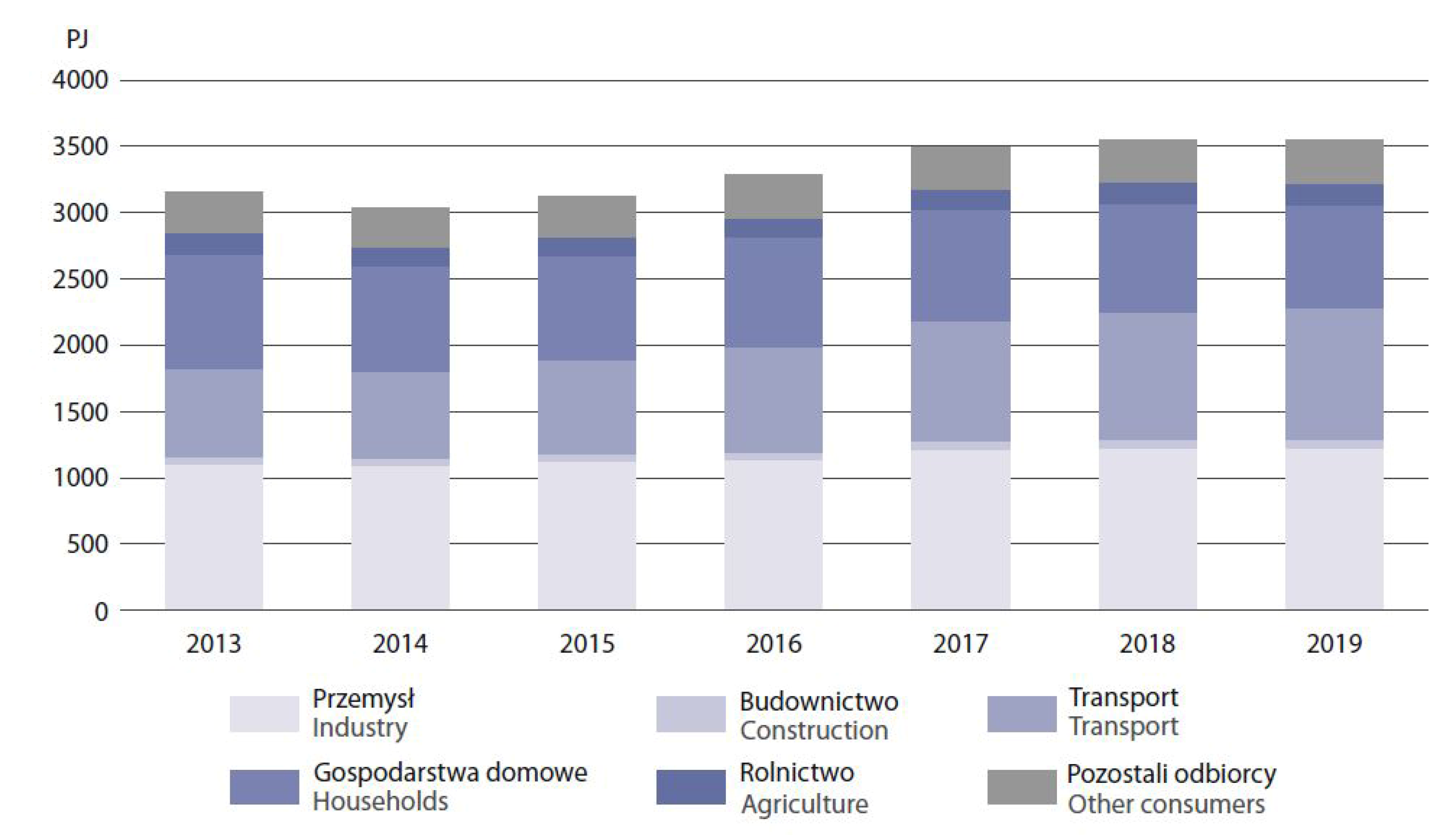
Figure 3.
Share of each region in Poland in a comprehensive study to analyze energy consumption in the building sector [19].
Figure 3.
Share of each region in Poland in a comprehensive study to analyze energy consumption in the building sector [19].

Figure 4.
Building prototypes from the ASHRAE 90.1 standard [74].
Figure 4.
Building prototypes from the ASHRAE 90.1 standard [74].

Figure 5.
Research workflow.

Figure 6.
Heating EUI (a) and cooling EUI (b) in building prototypes from 2020 to 2080; the numbers demonstrate relative changes of values for 2080 compared to 2020.
Figure 6.
Heating EUI (a) and cooling EUI (b) in building prototypes from 2020 to 2080; the numbers demonstrate relative changes of values for 2080 compared to 2020.

Figure 7.
Change in the thermal load of building prototypes in 2020–2080 categorized by heating and cooling share; numbers demonstrate relative changes of values for 2050 and 2080 compared to 2020.
Figure 7.
Change in the thermal load of building prototypes in 2020–2080 categorized by heating and cooling share; numbers demonstrate relative changes of values for 2050 and 2080 compared to 2020.

Figure 8.
The share of thermal load of building prototypes in 2020, 2050, and 2080.

Table 1.
A short description of the research case study.
| Country | City | Latitude | Longitude | Time Zone | KGC |
|---|---|---|---|---|---|
| Poland | Poznan | 52.42N | 16.83E | 1.00 | Cfb |
| Population | Elevation | Weather Data | Heating DB 99.6% | Cooling DB 0.4% | Cooling 0.4% MCWB |
| 533,830 | 302 (m) | 2004–2018 (TMY) | −14.27 °C | 29.77 °C | 19.22 °C |
Table 2.
Selected years of each month in the Poznan Typical Meteorological Year for the period of 2004–2018.
Table 2.
Selected years of each month in the Poznan Typical Meteorological Year for the period of 2004–2018.
| Location | Jan | Feb | Mar | Apr | May | Jun | Jul | Aug | Sep | Oct | Nov | Dec |
|---|---|---|---|---|---|---|---|---|---|---|---|---|
| Ławica Airport | 2016 | 2017 | 2009 | 2005 | 2007 | 2005 | 2013 | 2017 | 2015 | 2008 | 2012 | 2014 |
Table 3.
Technical description of the prototype envelope components.
| Building Types | U-Factor (W/m2K) | Solar Heat Gain Coefficient (SHGC) | |||||
|---|---|---|---|---|---|---|---|
| Roof | External Wall | Glazing | Glazing | ||||
| Window | Skylight | Window | Window | ||||
| Apartment | High-rise (BP1) | 0.18 | 0.31 | 2.65 | - | 0.43 | - |
| Mid-rise (BP2) | 0.18 | 0.31 | ti2.65 | - | 0.43 | - | |
| Hotel | Large (BP4) | 0.18 | 0.45, 0.51 | 2.65 | - | 0.43 | - |
| Small (BP5) | 0.18 | 0.31 | 2.65, 2.85 | - | 0.43, 0.29 | - | |
| Office | Large (BP6) | 0.18 | 0.51 | 2.65 | - | 0.43 | - |
| Medium (BP7) | 0.18 | 0.31 | 2.65 | - | 0.43 | - | |
| Small (BP8) | 0.15 | 0.29 | 2.65 | - | 0.43 | - | |
| Health | Hospital (BP3) | 0.18 | 0.45, 0.51 | 2.65 | - | 0.43 | - |
| Outpatient (BP9) | 0.18 | 0.31 | 2.65 | - | 0.43 | - | |
| Restaurant | Fast food (BP10) | 0.15 | 0.29 | 2.65 | - | 0.43 | - |
| Sit-down (BP11) | 0.15 | 0.31 | 2.65 | - | 0.43 | - | |
| Retail | Stand-alone (BP12) | 0.18 | 0.51 | 2.65 | 2.96 | 0.43 | 0.34 |
| Strip-mall (BP13) | 0.18 | 0.31 | 2.65 | - | 0.43 | - | |
| School | Primary (BP14) | 0.18 | 0.31 | 2.65 | - | 0.43 | - |
| Secondary (BP15) | 0.18 | 0.31 | 2.65 | 2.96 | 0.43 | 0.34 | |
| Warehouse | (BP16) | 0.21, 0.53 | 0.28, 0.47 | 2.65 | 2.96 | 0.43 | 0.34 |
Table 4.
Relative changes of weather parameters for 2050 and 2080 compared to 2020.
| Weather Parameters | 2020 | 2050 | 2080 |
|---|---|---|---|
| Dew point temperature (°C) | 4.2 | 6.0 | 7.2 |
| Average ground temperature (°C) | 8.0 | 10.8 | 12.6 |
| Dry bulb temperature (°C) | 8.2 | 10.9 | 12.6 |
| Direct normal radiation (Wh/m2) | 59.1 | 81.3 | 86.4 |
| Diffuse horizontal radiation (Wh/m2) | 75.9 | 72.5 | 71.4 |
| Global horizontal radiation (Wh/m2) | 109.7 | 113.0 | 115.7 |
| Horizontal infrared radiation (Wh/m2) | 303.0 | 322.1 | 331.5 |
| Direct normal illuminance (lux) | 7015 | 7385 | 7875 |
| Diffuse horizontal illuminance (lux) | 8578.5 | 8609.7 | 8527.7 |
| Global horizontal illuminance (lux) | 12,157 | 12,434 | 12,739 |
| Atmospheric pressure (Pa) | 101,325 | 101,272 | 102,249 |
| Relative humidity (%) | 78.1 | 74.6 | 72.7 |
| Total sky cover (0–10) | 4.5 | 4.2 | 4.3 |
Publisher’s Note: MDPI stays neutral with regard to jurisdictional claims in published maps and institutional affiliations. |
© 2021 by the authors. Licensee MDPI, Basel, Switzerland. This article is an open access article distributed under the terms and conditions of the Creative Commons Attribution (CC BY) license (https://creativecommons.org/licenses/by/4.0/).
Share and Cite
MDPI and ACS Style
Bazazzadeh, H.; Pilechiha, P.; Nadolny, A.; Mahdavinejad, M.; Hashemi safaei, S.s. The Impact Assessment of Climate Change on Building Energy Consumption in Poland. Energies 2021, 14, 4084. https://doi.org/10.3390/en14144084
AMA Style
Bazazzadeh H, Pilechiha P, Nadolny A, Mahdavinejad M, Hashemi safaei Ss. The Impact Assessment of Climate Change on Building Energy Consumption in Poland. Energies. 2021; 14(14):4084. https://doi.org/10.3390/en14144084
Chicago/Turabian StyleBazazzadeh, Hassan, Peiman Pilechiha, Adam Nadolny, Mohammadjavad Mahdavinejad, and Seyedeh sara Hashemi safaei. 2021. "The Impact Assessment of Climate Change on Building Energy Consumption in Poland" Energies 14, no. 14: 4084. https://doi.org/10.3390/en14144084
Note that from the first issue of 2016, this journal uses article numbers instead of page numbers. See further details here.