Wind Farm Power Optimization and Fault Ride-Through under Inter-Turn Short-Circuit Fault

Abstract

Inter-Turn Short Circuit (ITSC) fault in stator winding is a common fault in Doubly-Fed Induction Generator (DFIG)-based Wind Turbines (WTs). Improper measures in the ITSC fault affect the safety of the faulty WT and the power output of the Wind Farm (WF). This paper combines derating WTs and the power optimization of the WF to diminish the fault effect. At the turbine level, switching the derating strategy and the ITSC Fault Ride-Through (FRT) strategy is adopted to ensure that WTs safely operate under fault. At the farm level, the Particle Swarm Optimization (PSO)-based active power dispatch strategy is used to address proper power references in all of the WTs. The simulation results demonstrate the effectiveness of the proposed method. Switching the derating strategy can increase the power limit of the faulty WT, and the ITSC FRT strategy can ensure that the WT operates without excessive faulty current. The PSO-based power optimization can improve the power of the WF to compensate for the power loss caused by the faulty WT. With the proposed method, the competitiveness and the operational capacity of offshore WFs can be upgraded.

1. Introduction

In recent years, the development of offshore wind energy has been very rapid. The total installed offshore wind capacity has reached 22 GW [1]. However, the fault rate of offshore Wind Turbines (WTs) is high because of the harsh operating environment. At the same time, the special location of the installation makes the maintenance costs of offshore WTs high as well. The Operation and Maintenance (O&M) costs of offshore Wind Farms (WFs) are up to 25% to 40% [2]. These factors have greatly restricted the development of offshore wind energy.

As the main component that converts mechanical energy into electrical energy, the generator is critical to WTs. A fault of the generator directly affects the performance and the safety of the WT. Although the fault rate of the generator is not the highest, the downtime caused by the generator is quite long [3]. For offshore WTs, the same downtime means more power loss because of the high capacity of the offshore WT and the rich wind resource. However, not all faults require shutdown of the faulty WT. The measures corresponding to the fault should be analyzed in detail according to the specific characteristics and the severity of the fault to obtain the most appropriate response. By reducing the fault effect without shutting down, the competitiveness of offshore WTs is significantly improved. There are already some papers [4,5] about Fault-Tolerant Control (FTC) of WTs, but few of these focus on generator faults. The Inter-Turn Short Circuit (ITSC) fault of stator winding is one of the most common faults in generators. The impact of ITSC at the initial stage is not great. However, if the faulty WT continues to operate according to the control strategy as normal, the faulty current causes high temperatures in the faulty phase. The simulation of numerical modeling and experiment in [6] showed that an ITSC fault in the stator causes asymmetry of the stator currents. The current of the faulty phase is higher than that of the healthy phases. The difference in the stator currents became greater with the increase in shorted turns. As a rule of thumb, the insulation lifetime is reduced by half for each 10 °C that the motor temperature exceeds its rated insulation temperature [7]. An operation without considering fault may lead to the development of an ITSC fault or more serious faults, such as phase-to-ground and phase-to-phase short circuit. Currently, most research on ITSC faults of WTs is about Fault Detection and Diagnostics (FDD) [8]. FDD is realized through the acquisition and processing of signals including vibration, noise, torque, temperature, current, voltage, etc. For faults of a generator, the method based on electrical signals has been proven to be more effective [9]. Most recent work about active power dispatch were proposed to maximize the power output of wind farms [10], to optimize the power-tracking performance [11,12], to alleviate the fatigue of WTs [12], and to balance the fatigue distribution of WFs [10]. However, none take the fault condition of generator into account. Without consideration of the fault effects, there are two direct ways to deal with ITSC faults: one is the Safety-First Strategy (SFS), which directly shuts down the faulty WT; the other is Power-First Strategy (PFS), which ignores the fault and continues to operate the faulty WT as normal. SFS can completely protect the fault WT, while it causes unnecessary power loss for low-severity faults. On the contrary, although PFS can avoid power loss, long-term operation in a fault condition may lead to the development of faults. The obvious phenomenon of an ITSC fault is the increase in currents in the faulty phase [13]. In practice, the excessive current triggers the WT’s safety alarm and causes the shutdown of the faulty WT directly. Therefore, PFS is only used to analyze and compare the impact of different strategies on WTs and WFs for an ITSC fault. If the faulty current cannot exceed the rated current through WT regulation, the excessive temperature of the winding in the faulty phase can be avoided. This means that the faulty WT can continue to operate safely in this condition. Therefore, a derating operation of the faulty WT is another option to deal with ITSC faults.

The power optimization of WFs is very important as well. The inflow wind of the downstream WTs is affected by upstream WTs because of the wake effects [14]. This aerodynamic interaction among WTs diminishes the power performance of the WF. An appropriate power optimization method can directly improve the power output and can further compensate for the power loss caused by a derated faulty WT. Compared with the layout optimization of WFs, the power optimization through active wake control is more feasible in improving the power generation capacity of existing WFs [15]. Prevalent wind farm control concepts include axial induction-based control and yaw-based wake redirection [16]. Axial induction-based control (also named power derating) reduces the axial induction factor of upstream WTs by pitch and rotor speed adjustment. This means the upstream WTs operate in the derating mode. With the decrease in thrust force of the upstream WTs, the power loss of the upstream WTs can be outweighed by the power gain in the downstream WTs [17]. It should be noted that different derating strategies have disparate impacts on WTs. Yaw-based wake redirection control deflects the wake flow away from the rotor of the downstream WTs by operating the upstream WTs with nacelle yaw misalignment. As a newer method, its effectiveness has been verified by both Large-Eddy Simulation (LES) and field tests [18]. However, the defect of this method is that an improper yaw angle causes an increase in the fatigue loads of WTs [19]. Moreover, the yaw system may not be able to track the yaw angle reference in time because of its long response time. Here, we adopt the first concept for power optimization because the ITSC Fault Ride-Through (FRT) is related to the derating as well. The Minimum Thrust Coefficient (Min-$C_{\mathrm{t}}$) strategy is used in the healthy WTs to obtain more power for the WF. Regarding the derating of the WT, the derating strategy that has a significant impact on the performance of the WT and the WF has to be considered. The most commonly used derating strategy is Maximum Rotor Speed (Max-$\omega$). When the WT is downregulated under the Max-$\omega$ strategy, the rotor speed is adjusted to the maximum value. The rotating rotor stores the maximum kinetic energy and can react to the increased power reference quickly. The Min-$C_{\mathrm{t}}$ strategy is another strategy that can minimize the wake effect on downstream WT by minimizing the thrust coefficient. More details about the Max-$\omega$ and Min-$C_{\mathrm{t}}$ strategies are given in Section 3.1.

The main contribution of this paper is the reduction in impacts of an ITSC fault on a faulty WT and the WF through the combination of control at the turbine level and optimization at the farm level. The selection of a derating strategy can avoid negative impacts on the faulty WT due to improper derating strategies. The ITSC FRT strategy can derate a faulty turbine to avoid the faulty current from exceeding the rated current without knowing the fault level and the corresponding power limit. Finally, power dispatch optimization with the Min-$C_{\mathrm{t}}$ strategy can reduce the power loss caused by a derated faulty WT. It should be noted that the proposed method is only suitable for the initial stage of an ITSC fault because the excessive derating corresponding to the high fault level has a negative impact on the WT. On the premise that the ITSC fault can be accurately detected, a time judgment should be added to the overcurrent safety trigger condition under this fault. That is, when an ITSC fault is detected, if a faulty WT can automatically reduce the fault current to a safe value within a certain period of time, the WT will not shut down.

To implement the reliable WF operation, this paper proposes an active power dispatch optimization method considering the stator ITSC faults of a Doubly-Fed Induction Generator (DFIG). The general idea is to take different measures at the turbine level and the farm level to minimize the fault effect as much as possible. At the turbine level, the faulty turbine is operated in the derating mode. At the same time, the derating strategy of the faulty WT is switched from the Min-$C_{\mathrm{t}}$ strategy to the Maximum Rotor Speed (Max-$\omega$) strategy to protect the faulty generator. The ITSC FRT strategy is used to realize the derating operation through Proportional-Integration (PI) adjustments of the references of the pitch angle and the generator torque. The objective is to prevent the faulty stator current from exceeding the rated current value. At the farm level, the active power dispatch is formulated as a multi-objective problem and optimized by the Particle Swarm Optimization (PSO) algorithm.

The paper is organized as follows: Section 2 describes the wind farm model, Section 3 presents the control strategy at the turbine level under ITSC fault, Section 4 presents the active power dispatch optimization, and Section 5 presents the simulation results and the analysis. The paper is concluded in Section 6.

2. Wind Farm Model

The wind farm model includes three main parts: the wake model, the wind turbine model, and the layout. The wake model is essential for the study of wind farm power because of the aerodynamic interaction among WTs. The wind turbine model includes a dynamic model and a static model. The dynamic model is adopted for the ITSC FRT strategy. The static model is used for power dispatch optimization. As an important property of the WF, the layout has a significant effect on wakes. These three parts are described below.

2.1. Wake Model

The wake effect is the aerodynamic interaction among WTs in the WF. The properties of the inflow wind of the downstream WT change due to the influence of the upstream WTs when the inflow wind passes the upstream WTs and blows to the downstream WT. The two main effects of the wake effect are the wind velocity deficit and the increase in turbulence. The wind velocity deficit directly affects the power performance of the entire WF. This paper focuses on the active power optimization of WFs, so only the wind velocity deficit is considered. To describe the wake effects, many different wake models are proposed by different researchers [20]. Among these models, the Jensen wake model is most widely used for a single wake and the quadratic summation method is often used for multiple wakes. Although the accuracy is lower compared with the CFD model, the simple calculation is very suitable for online computation and control. The expression of the Jensen model is given by [20]

$$\frac{v}{u}=\frac{1-\sqrt{1-C_{\mathrm{t}}}}{{(1+2\alpha X/D)}^2},$$

(1)

where v is the wind speed of the downstream WT; u is the ambient free wind speed; $C_{\mathrm{t}}$ is the thrust coefficient of the upstream WT; X is the distance between the upstream and the downstream WTs; D is the diameter of the rotor of the turbine; and $\alpha$ is the decay constant, which chooses 0.05 for offshore WFs [21].

The quadratic summation method for multiple wakes can be expressed by [20]

$${(1-\frac{v_j}{u})}^2=\sum _{i=1}^m{(1-\frac{v_{ij}}{u})}^2,$$

(2)

where $v_j$ is the wind speed of the jth WT, m is the number of wakes that the jth WT is in, and $v_{ij}$ is the wind speed of the jth WT under the influence of the wake of the ith WT.

It can be seen from the wake model that $C_{\mathrm{t}}$ directly affects the wake effect except the factors determined by the WF. The higher $C_{\mathrm{t}}$, the greater the wind velocity deficit of the downstream WT and the less the power that can be produced. In addition, some reduced-order wake models [22] can obtain a relatively good accuracy at a lower computational cost compared with high-fidelity wake models. The choice of the wake model affects the computational time, the complexity of the optimization and the control methods.

2.2. Wind Turbine Model

The operation of a WT can be divided into two modes according to the power condition. The first is the normal mode, and the other is the derating mode. The WT operates in the normal condition and produces power as the power curve in the normal mode. In the derating mode, the power reference is lower than the corresponding power value on the WT’s designed power curve. Therefore, the turbine controller downregulates the WT. In this situation, different strategies can be adopted. The value of $C_{\mathrm{t}}$ is different in different derating strategies as well. Among them, the Max-$\omega$ strategy is the most widely used. The Min-$C_{\mathrm{t}}$ strategy can minimize the $C_{\mathrm{t}}$. Therefore, we adopt these two strategies from the perspective of fault protection and WF power optimization. The reasons will be explained below. In addition, the WT static model adopted here is based on the modified NREL 5 MW WT in the SimWindFarm Simulink toolbox [23]. The structure of the WT model is shown is Figure 1.

For the ITSC FRT strategy, a dynamic model of the WT is required. Since the generator model SimWindFarm is very simple, we replace it with a DFIG model. The mathematical model of DFIG adopted is the classic state-space model in an $\alpha$$\beta$ stationary reference frame. The relevant parameters are listed in Table 1 in Section 5. The specific model description is presented in [24]. However, the dynamic model is not suitable for the subsequent optimization calculation of a power dispatch, which greatly increases the calculation time. Therefore, we extracted the values of the power output and the thrust coefficient at different fault levels after being protected to form a static model of faulty WTs under the ITSC FRT strategy.

2.3. Wind Farm Layout

The spacing between WTs has a direct effect on the wake. This can be seen from the wake model. The larger the spacing, the smaller the wake effect. However, a too large spacing leads to an increase in investment costs. The typical spacing range for an offshore WF is from 5D to 15D [25], where D is the diameter of the turbine rotor. The WF layout adopted in this paper is shown in Figure 2. Five WTs were arranged in a straight line with 6.5D spacing. The wind direction was ${270}^{\circ }$, which means the downstream WTs were in the full wake condition. Figure 3 shows the distribution of the wind speed in this WF. The inflow wind speed was 12 m/s. The decrease in the wind speed is quite small after the fourth WT. Therefore, the WF with five WTs is sufficient to express the impacts on power output caused by wake effect. Since the proposed approach is based on PSO at the wind farm level, application in the scenario for deep array layouts does not need any special modification. However, the depth of the array affects the calculation time. Therefore, it is necessary to adjust the parameters of the PSO algorithm.

3. Control Strategy at the Turbine Level under ITSC Fault

The control strategy for normal WTs cannot protect a faulty turbine under fault conditions. Therefore, we adopt the ITSC FRT strategy proposed in [24]. The fault detection method is based on a closed-loop state observer [26]. By combining the fault model of the DFIG under stator ITSC and the closed-loop state observer, the residual value equation of the current can be obtained. According to the residual value equation, the occurrence of a fault can be detected. When an ITSC fault occurs, the WT adopts the Max-$\omega$ downregulation strategy. The difference between the fault phase current and the rated current is superimposed on the generator torque reference through a PI operation to reduce the power of the faulty WT until the fault current is not greater than the rated current value.

It should be noted that this ITSC FRT strategy does not need to estimate the fault degree. Therefore, it not only can lower the requirement of the fault detection but also can avoid improper power limitation caused by the estimation errors. In addition, the accuracy of the fault detection method is very important. If the fault cannot be detected in time, the fault degree increases.

3.1. Switching the Derating Strategy

3.1.1. Max-$\omega$ Strategy

The most commonly used derating strategy is the Max-$\omega$ strategy. When the WT needs to operate in the derating mode, the rotor speed increases to or maintains the maximum rotor speed. Then, the power output is adjusted to the specific reference by pitch angle. The Max-$\omega$ strategy has many advantages. Since the rotor speed is kept at the maximum value, the rotor stores the maximum kinetic energy. When the power reference increases, the WT can respond very quickly. In addition, the rotor speed also has a great influence on the current of DFIG. The effective value of the stator current can be expressed as

$$I_{\mathrm{s}}=\frac{P_{\mathrm{s}}}{\sqrt{3}{U}_{\mathrm{s}}cos\varphi }=\frac{P}{\sqrt{3}{U}_{\mathrm{s}}(1-s)cos\varphi },$$

(3)

where $P_{\mathrm{s}}$, $U_{\mathrm{s}}$, P, $\varphi$, and s are the stator power, stator voltage, power output, phase angle, and slip, respectively. Slip is defined as

$$s=\frac{{\omega }_{\mathrm{s}}-{\omega }_{\mathrm{e}}}{{\omega }_{\mathrm{s}}},$$

(4)

where ${\omega }_{\mathrm{s}}$ is the synchronous electrical angular speed and ${\omega }_{\mathrm{e}}$ is the rotor electrical angular speed.

It can be seen from the expression that, the higher the speed, the less power the stator emits and the lower the effective current in stator. Therefore, the Max-$\omega$ strategy can decrease the stator current when excessive stator current-related fault occurs.

3.1.2. Min-$C_{\mathrm{t}}$ Strategy

The Min-$C_{\mathrm{t}}$ strategy can be used in the derating mode to reduce the wake effects on the WF power. The strategy used in this paper was proposed in [27]. The process is shown in Figure 4. It can be seen that Min-$C_{\mathrm{t}}$ is executed at the turbine level. When the turbine is in the derating mode, the $C_{\mathrm{p}}$ value is calculated first at the current power reference and wind speed. Then, the minimum $C_{\mathrm{t}}$ is selected from all of the operating points at a specific $C_{\mathrm{p}}$. Finally, this minimum $C_{\mathrm{t}}$ operating point is set as the reference to the WT controller. It should be noted that the minimum $C_{\mathrm{t}}$ operating point usually uses a low rotor speed. Therefore, the limitation of the rotor speed is necessary. Two factors need to be considered: one is the designed minimum rotor speed of the WT, and the other is that the stator current corresponding to the rotor speed should not exceed the rated value. Figure 5 shows the operating points of the WT with the Max-$\omega$ and Min-$C_{\mathrm{t}}$ strategies. The thick line is the $C_{\mathrm{p}}$ curve at a specific value. The square corresponds to the operating point under the Max-$\omega$ strategy, and the circle corresponds to the operating point under the Min-$C_{\mathrm{t}}$ strategy. These two points are on the same $C_{\mathrm{p}}$ curve, so their $C_{\mathrm{p}}$ values are the same. However, these two points are on two different $C_{\mathrm{t}}$ curves. The $C_{\mathrm{t}}$ value of the operating point under the Min-$C_{\mathrm{t}}$ strategy is less than that under the Max-$\omega$ strategy. Therefore, when the WT produces the same power, the $C_{\mathrm{t}}$ value is smaller under the Min-$C_{\mathrm{t}}$ strategy. This means that the wake effect behind this WT is smaller.

According to the wake model, we can see that the WT using the Min-$C_{\mathrm{t}}$ strategy is more conducive to improving the power of the WF. However, the rotor speed is usually small in this strategy. Equation (3) shows that, if the rotor speed becomes smaller, the effective current in stator increases with the same power. This situation is harmful to the generator under ITSC fault. If the faulty WT continues to use the Min-$C_{\mathrm{t}}$ strategy, the power output is correspondingly reduced under the premise of ensuring that the fault phase current does not exceed the rated value. That means more power loss.

Therefore, the Min-$C_{\mathrm{t}}$ strategy is more suitable for healthy WTs to improve the WF power. When an ITSC fault is detected, the derating strategy of the faulty WT should be switched from Min-$C_{\mathrm{t}}$ to Max-$\omega$.

3.2. Fault Ride-Through Strategy

Generally, the operation of WTs is divided into four regions, as shown in Figure 6, according to the wind speed and the rotor speed. The detail can be found in [28]. These four regions are as follows:

• Minimum speed operation region
• Maximum Power Point Tracking (MPPT) region
• Maximum speed in partial load region
• Maximum speed in rated power region

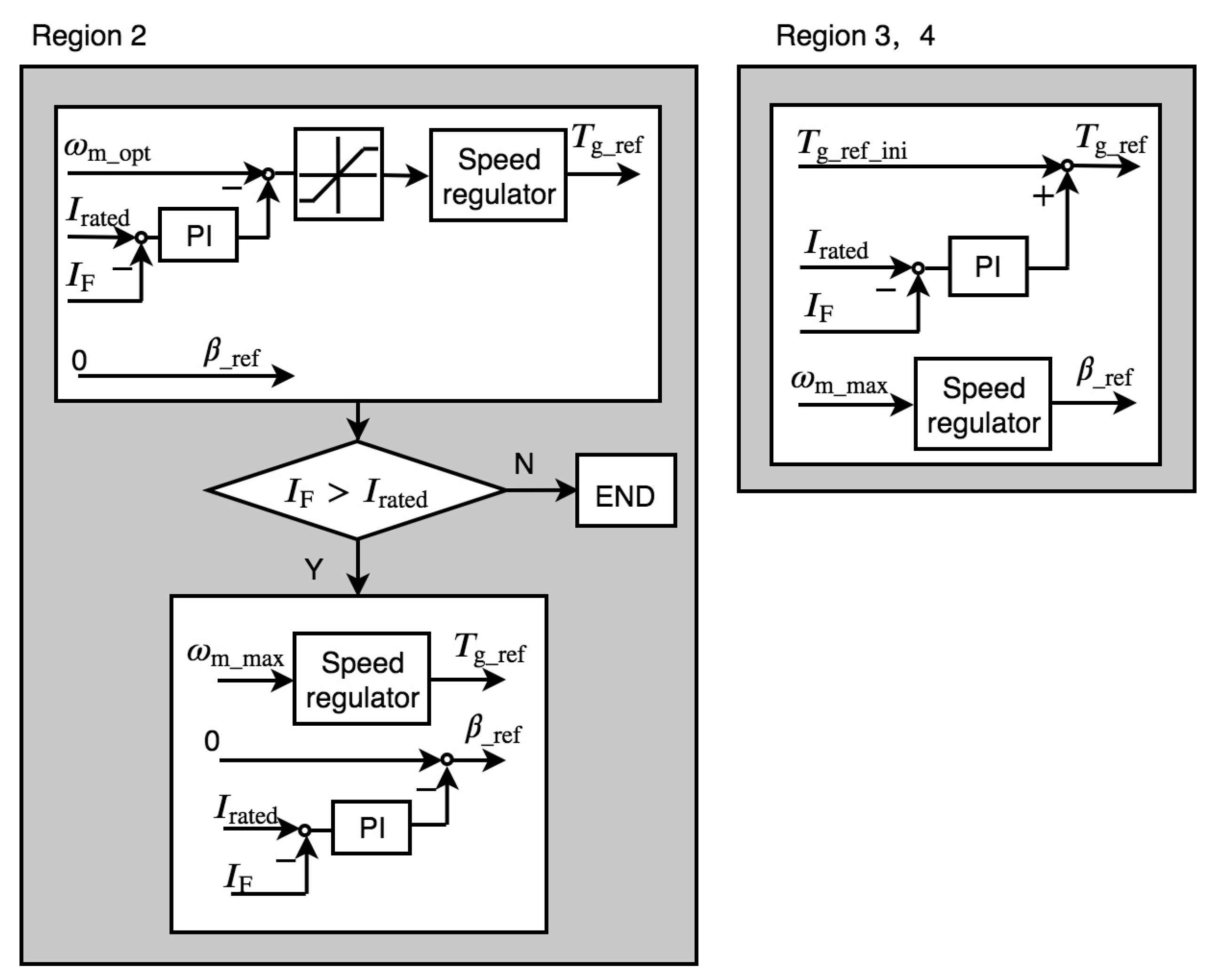
One of the main fault effects is the increase in the winding temperature caused by the faulty current. The excessive current leads to further deterioration of the insulation layer. Therefore, the ITSC FRT strategy takes different actions in the four operation regions to avoid the faulty current from exceeding the rated current value. A flowchart of regions 2, 3, and 4 is shown in Figure 7.

When the faulty current is lower than the rated current, the WT operates as the normal control strategy. When the faulty current is higher than the rated current, the control action depends on the operation region.

In region 1, the WT still operates according to the normal control strategy. Since the load of the generator is small, the faulty current does not exceed the rated current.

In region 2, the pitch angle is set to 0, and the current difference between the faulty current and the rated current is superimposed on the rotor speed reference to the speed regulator through PI control. The output of the speed regulator is set as the generator torque reference. If the faulty current still exceeds the rated current, the current difference calculated through PI control is set as the pitch angle reference. At the same time, the maximum rotor speed is set as the reference to the speed regulator.

In regions 3 and 4, the current difference calculated through PI control is superimposed onto the generator torque reference and the maximum speed is set as the reference to the speed regulator. The output of the speed regulator is set as the pitch angle reference.

The basic idea of the ITSC FRT strategy is to downregulate the faulty WT by adjusting the reference of the generator torque and the pitch angle based on operational characteristics in the different regions. The derating level depends on the faulty current. With this ITSC FRT strategy, the faulty WT can continue to operate in a safe condition when an ITSC fault occurs in stator winding.

4. Power Optimization at the Farm Level under ITSC Fault

Active power dispatch of WFs impacts the power performance of WFs due to the wake. Therefore, the reasonable power dispatch can improve the WF power. The conventional Proportional Dispatch Strategy (PDS) distributes the power demand from the Transmission System Operator (TSO) to all of the WTs according to the avaiable power ratio of each WT, which can be expressed by [23]

$$P_{\mathrm{r},i}=\frac{P_{\mathrm{a},i}}{{\sum }_{i=1}^n{P}_{\mathrm{a},i}}{P}_{\mathrm{dem}},$$

(5)

where $P_{\mathrm{r},i}$ represents the power reference of the ith WT, $P_{\mathrm{a},i}$ represents the available power of the ith WT, and $P_{\mathrm{dem}}$ represents the power demand from TSO.

However, PDS does not take the reduction of wake effects into account. Regarding to the fault condition, SFS and PFS mentioned in Section 1 can be expressed by

$$P_{\mathrm{r},\mathrm{f}}=\left\{\begin{array}{cc}0,\hfill & \mathrm{in}\mathrm{SFS},\\ P_{\mathrm{r},i},\hfill & \mathrm{in}\mathrm{PFS}.\end{array}\right.$$

(6)

where $P_{\mathrm{r},\mathrm{f}}$ represents the power reference of the faulty WT.

It can be seen that the severity of the fault is not considered in SFS and PFS. Therefore, this paper adopts PSO-based Optimal Power Dispatch Strategy (OPDS) with ITSC FRT strategy to take wake effects and fault condition into consideration.

The first objective of power dispatch is to track the power demand from TSO. Since PSO is used as a heuristic optimization algorithm, the power fluctuation should be considered. Otherwise, the power reference could vary a lot due to the change in the optimization result, which affects the health of WTs. Moreover, WTs cannot produce power that is higher than the available power. Therefore, all power references greater than the available power correspond to the same power output. This characteristic of the WT makes the optimization process easily fall into a local optimum.

Therefore, the active power dispatch is programmed as a multi-objective. The objective function is formulated as the following to solve the problem:

$$\begin{array}{cc}\hfill min& \{\frac{|{\sum }_{i=1}^n{P}_i\left(k\right)-P_{\mathrm{dem}}\left(k\right)|}{P_{\mathrm{dem}}\left(k\right)}·k_1+[1-\mathrm{r}[\mathit{P}(k-1),\mathit{P}\left(k\right)]]·k_2+\frac{{\sum }_{i=1}^n|P_{\mathrm{r},i}\left(k\right)-P_i\left(k\right)|/P_{\mathrm{r},i}\left(k\right)}{n}·k_3\}\hfill \\ \\ \hfill & s.t.0\le P_{\mathrm{r},i}\left(k\right)\le P_{\mathrm{rated}}.\hfill \end{array}$$

(7)

where n is the number of WTs, k is the discrete time index, $P_i$ is the power output of the ith WT, $P_{\mathrm{dem}}$ is the power demand from TSO, $\mathit{P}$ is the power output vector of WTs, $P_{\mathrm{r},i}$ is the power reference of the ith WT, and $k_1$, $k_2$ and $k_3$ are the weight coefficients.

It can been seen that the objective function consists of three terms according to different goals. The first term represents the difference between the power demand and the power output of the WF and should be as small as possible. Since this is the main target of the WF controller, the corresponding weight coefficient $k_1$ should be greater than $k_2$ and $k_3$.

The second term can avoid the power fluctuation caused by the randomness process in PSO. This power fluctuation is not the dynamic power change of WTs but the power change of the WTs at the adjacent time. The correlation coefficient is expressed by

$$\mathrm{r}[\mathit{P}(k-1),\mathit{P}\left(k\right)]=\frac{\mathrm{cov}\left(\mathit{P}\right(k-1),\mathit{P}(k\left)\right)}{\mathrm{std}\left[\mathit{P}\right(k-1\left)\right]·\mathrm{std}\left[\mathit{P}\right(k\left)\right]},$$

(8)

where $\mathrm{cov}[{\mathit{P}}_i\left(k\right),\mathit{P}(k-1)]$ is the covariance of $\mathit{P}\left(k\right)$ and $\mathit{P}(k-1)$ and where $\mathrm{std}\left[\mathit{P}\right(k\left)\right]$ and $\mathrm{std}\left[\mathit{P}\right(k-1\left)\right]$ are the standard deviations of $\mathit{P}\left(k\right)$ and $\mathit{P}(k-1)$.

The third term can prevent the PSO from falling into a local optimum due to the factor mentioned above. The detail explanation of the objective function can be found in [29]. However, the difference between these two objective functions is that the power limitation of the faulty WT does not need to be calculated. Since the power limitation has been implemented by the ITSC FRT strategy at the turbine level, there is no need to repeat this consideration in the power dispatch process. During the PSO process, when the faulty WT cannot track the reference value, the WF controller automatically reduces the power reference during the next iteration due to the existence of the third term. The control diagram of the WF power dispatch is shown in Figure 8.

It should be noted that the computational cost of the optimization process mainly depends on the fidelity of the wake model. Although the high-fidelity wake model has a more accurate estimation of the wake, its excessively high computational cost can hardly be used in the actual controller. The simple analytical model adopted in the paper is more suitable for offshore WF control due to its low computational cost (∼${10}^{-3}$ CPU hours per simulation) [30]. The CPU used in this study was Intel I5 2.8 GHz. The calculation time of active power dispatch optimization for five WTs case was about 4 s when the iteration number was set to 50 and the population size was set to 60. This calculation time can be further reduced on faster processors or through parallel computing. In actual WFs, the power reference time interval varies from seconds to minutes. The effect of an ITSC fault was temperature-induced, which is a slow process at the early stages of a fault. Therefore, the calculation time of the online optimization does not affect the fault protection. To investigate the robustness of the controller, one should investigate the turbine level controller. In fact, the wind farm level control distributes the optimal power reference as the set point for the turbine level controller. Thus, the wind farm level controller does not change the robust stability and performance of the turbine level controller.

5. Simulations

The simulations of the WF mentioned in Section 2 under fault-free and fault conditions were performed to verify the effectiveness of the proposed method. The parameters of the DFIG are listed in Table 1.

Table 1. Parameters of five MW DFIG wind turbines.

Parameter	Value
Rated Power	5 MW
Rotor Diameter	126 m
Min. and Max. Rotor Speed	6.9 rpm, 12.1 rpm
Cut-In, Rated, Cut-Out Wind Speed	3 m/s, 11.4 m/s, 25 m/s
Gearbox Ratio	97:1
Synchronous Frequency	50 Hz
Stator Resistance	1.08 m$\mathsf{\Omega }$
Rotor Resistance	1.22 m$\mathsf{\Omega }$
Stator Leakage Inductance	0.12 mH
Rotor Leakage Inductance	0.21 mH
Magnetizing Inductance	2.8 mH
Number of Pole-Pairs	3

Table 1. Parameters of five MW DFIG wind turbines.

Parameter	Value
Rated Power	5 MW
Rotor Diameter	126 m
Min. and Max. Rotor Speed	6.9 rpm, 12.1 rpm
Cut-In, Rated, Cut-Out Wind Speed	3 m/s, 11.4 m/s, 25 m/s
Gearbox Ratio	97:1
Synchronous Frequency	50 Hz
Stator Resistance	1.08 m$\mathsf{\Omega }$
Rotor Resistance	1.22 m$\mathsf{\Omega }$
Stator Leakage Inductance	0.12 mH
Rotor Leakage Inductance	0.21 mH
Magnetizing Inductance	2.8 mH
Number of Pole-Pairs	3

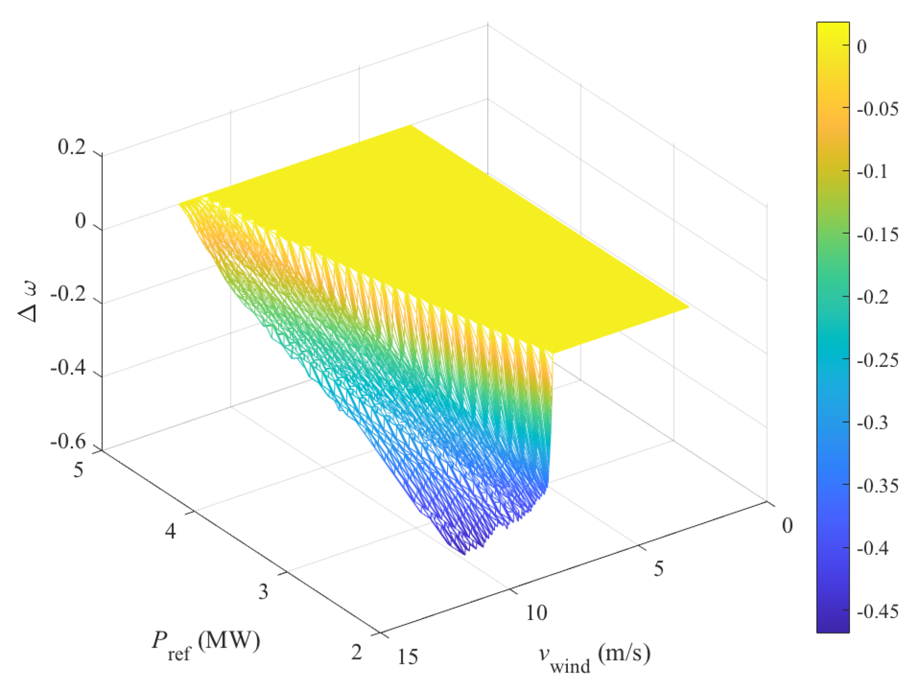
First, we compare the rotor speed and the $C_{\mathrm{t}}$ in Max-$\omega$ and Min-$C_{\mathrm{t}}$ strategies. The results are shown in Figure 9 and Figure 10. The wind speed range was from 3 to 14 m/s, and the power reference range was from 2 to 5 MW. The figures show that the different impacts of the derating strategies on the WT are mainly reflected in rotor speed and $C_{\mathrm{t}}$ in the region of low power reference. Here, we use $\Delta \omega$ and $\Delta C_{\mathrm{t}}$ to show the impacts on the rotor speed and $C_{\mathrm{t}}$ under different derating strategies. The definitions are as follows.

$$\left\{\begin{array}{c}\Delta \omega ={\omega }_{\_\mathrm{Min}-{\mathrm{C}}_{\mathrm{t}}}-{\omega }_{\_\mathrm{Max}-\omega }\hfill \\ \Delta C_{\mathrm{t}}=C_{\mathrm{t}\_\mathrm{Min}-{\mathrm{C}}_{\mathrm{t}}}-C_{\mathrm{t}\_\mathrm{Max}-\omega },\hfill \end{array}\right.$$

(9)

where ${\omega }_{\_\mathrm{Min}-{\mathrm{C}}_{\mathrm{t}}}$ and ${\omega }_{\_\mathrm{Max}-\omega }$ are the rotor speeds under the Min-$C_{\mathrm{t}}$ and Max-$\omega$ strategies and where $C_{\mathrm{t}\_\mathrm{Min}-{\mathrm{C}}_{\mathrm{t}}}$ and $C_{\mathrm{t}\_\mathrm{Max}-\omega }$ are the thrust coefficients under the Min-$C_{\mathrm{t}}$ and Max-$\omega$ strategies.

In Figure 9, $\Delta \omega$ is large in the region of low power reference and high wind speed. However, $\Delta C_{\mathrm{t}}$ in Figure 10 is not large when the wind speed is high. That is because the value of $C_{\mathrm{t}}$ depends on TSR and the pitch angle. TSR is not only affected by the rotor speed but also by the wind speed. According to the definition, TSR is proportional to the rotor speed and inversely proportional to the wind speed. In the high wind speed region, TSR is very small. It can be seen from Figure 5 that the $C_{\mathrm{t}}$ curves are denser when TSR is small. That means the change rate of $C_{\mathrm{t}}$ is small in the high wind speed region. Therefore, $\Delta C_{\mathrm{t}}$ is not as small as $\Delta \omega$ in the high wind speed region.

5.1. Power Optimization of Wind Farm under Fault-Free Condition

In this case, the power outputs of all of the WTs under different derating strategies and different power dispatch strategies are compared. It should be noticed that the power optimization of wake effects is beneficial at low wind speeds. If the wind speed of the last WT is still above the rated wind speed under wake effects, the effect of the power optimization is minimal. Therefore, the wind speed is set to 12 m/s. When the power demand is greater than the available power of the wind farm, wind turbines work based on maximum power point tracking. Thus, for the baseline, the power demand is set to 20 MW. All of the WTs adopted only one type of derating strategy in each simulation. The values of $k_1$, $k_2$, and $k_3$ were obtained after many simulation tests to meet the power dispatch requirements. Finally, 10, 4, and 3 were selected, respectively. The simulation results are shown in

Table 2. Wind farm power with different strategies.

Derating Strategy Dispatch Strategy	Max-$\mathit{\omega }$ PDS $\mathit{P}\left(\mathbf{MW}\right)$	Max-$\mathit{\omega }$ OPDS $\mathit{P}\left(\mathbf{MW}\right)$	Min-${\mathit{C}}_{\mathbf{t}}$ OPDS $\mathit{P}\left(\mathbf{MW}\right)$
WT1	5.00	5.00	5.00
WT2	4.17	3.72	3.70
WT3	3.11	3.31	3.30
WT4	2.84	3.41	3.40
WT5	2.76	3.40	3.56
$P_{\mathrm{WF}}$	17.88	18.84	18.96

and Figure 11. It can be seen that the power of the WF is the highest with the Min-$C_{\mathrm{t}}$ strategy at the turbine level and with OPDS at the farm level. The results show that OPDS can improve the WF power because of the consideration of the wake effects. The adoption of the Min-$C_{\mathrm{t}}$ strategy further increases the WF power by reducing $C_{\mathrm{t}}$.

5.2. Fault Ride-Through under Fault Condition

To simulate the ITSC fault on stator winding, a 10% short circuit fault on phase A was performed at t = 30 s. The ITSC FRT strategy was used at t = 35 s. The wind speed was 12 m/s. The waveforms of the main variables of the faulty generator are shown in Figure 12. Figure 13 shows the transient currents of three phases at a faulty time and the current of a faulty phase A under ITSC FRT. When the fault occurred, the current of the faulty phase increased significantly. At t = 35 s, the ITSC FRT stratgy was used to reduce the faulty current. The generator torque decreased from 40.68 KN·m to 21.15 KN·m to derate the WT. At the same time, the pitch angle increased from 4.7 degrees to 9.3 degrees. Finally, the faulty WT was derated from 5 MW to 2.60 MW, and the effective value of the faulty current was reduced to the rated value after 20 s.

Last, the proposed method was compared with SFS and PFS. In this case, the wind speed was 12 m/s and the power demand was 20 MW. A 10% ITSC fault occurred on the second WT. The derating strategy of all WTs in SFS and PFS and of the healthy WTs in OPDS was the Min-$C_{\mathrm{t}}$ strategy to obtain more power. The faulty WT used the Max-$\omega$ strategy and FTR strategy to obtain more operational capacity. The result is shown in

Table 3. Power and faulty phase current under the SFS, PFS, and ITSC FRT strategies.

Strategy	SFS P(MW)	PFS P(MW)	ITSC FRT P(MW)
WT1	5.00	5.00	5.00
WT2	0	3.70	2.60
WT3	4.70	3.30	4.10
WT4	3.50	3.40	3.50
WT5	3.39	3.56	3.40
$P_{\mathrm{WF}}$	16.59	18.96	18.59
$I_{\mathrm{Fault}}$ (A)	0	3296	2507

. It can be seen that the faulty WT was shut down in SFS, operated as normal in PFS, and derated in the proposed strategy. The corresponding faulty currents were different as well. Although the power of the faulty WT was high in PFS, the current was much greater than the rated value. This would lead to further damage of the faulty phase. In contrast, the power using SFS was the smallest. The ITSC FRT strategy made the faulty WT continue operating without exceeding the rated current value of 2507 A. From the perspectives of protecting faulty units and of minimizing power loss, ITSC FRT is the most reasonable strategy.

ITSC FRT protects the faulty WT based on the faulty phase current at the turbine level. Compared with the method based on fault level estimation at the farm level in [31], the advantage of ITSC FRT is that the ITSC FRT strategy does not include an estimation of the fault level. Therefore, there are neither estimation errors nor negative effects on the final protection. To clearly observe the influence of the estimation error on the WT, we studied the following case. The wind speed was 12.5 m/s, and the wind direction was ${270}^{\circ }$. The power demand was 15 MW. Three WTs were arranged in a straight line with 6.5D spacing. An ITSC fault with an actual fault level of 8% occurred on the third WT. The downregulation strategy adopted here was Max-$\omega$.

Table 4. Comparison between ITSC FRT and the method based on fault level estimation.

Method	Estimated Fault Level	Power Limitation (MW)	WF Power (MW)	Difference between Faulty Phase Current and Rated Current (A)
ITSC FRT	-	3.55	13.37	0
Fault level estimation based	7%	3.88	13.70	+125
Fault level estimation based	9%	3.13	12.95	−510

shows the comparison between ITSC FRT and the method based on fault level estimation when the fault level is incorrectly estimated.

It can be seen that, when the estimated fault level is lower than the actual fault level, the value of the power limitation is higher than what it should be. The faulty current is still larger than the rated current. On the contrary, if the estimated fault level is higher than the actual fault level, the maximum power of the faulty WT is excessively reduced. The impact of the reduced power on the WF power is also affected by the location of the faulty WT. If the location of the faulty WT is upstream, the excessively reduced power may not have too much impact on the total power of the WF because of the reduced wake effects. However, if the faulty WT is downstream, the total power of the WF is reduced.

6. Conclusions

This paper investigates wind turbine control and wind farm optimization under an ITSC fault in DFIG stator winding. The following conclusions can be drawn from the present study. First, different derating strategies have different effects on the currents of WTs and on the power outputs of WFs. The Min-$C_{\mathrm{t}}$ strategy can improve the power output of WFs under fault-free condition, while the Max-$\omega$ strategy is more suitable for faulty WTs. Second, the ITSC FRT strategy can prevent faulty phase currents of WTs from exceeding the rated current. Due to the protection from the ITSC FRT strategy, fault conditions do not need to be considered again in the optimization process at the farm level. Third, the combination of turbine level control and farm level optimization is more conducive to improving the WF power. In addition, the proposed method is only suitable for the initial stage of the fault. When the severity is high, the faulty WT should be shut down in time according to the safety design of the WT. During faulty operation, the various operating parameters of the generator and the WT need to be more strictly monitored to prevent the fault from causing further serious consequences.

The findings of this study have a number of important implications for enhancing the fault operation capacity of WTs and for reducing the maintenance costs of WFs. The method of reducing the impact of faults by a derating operation can also be applied to other heat-related generator faults. The effects of the derating strategy, other generator faults, and the yaw-based control will be studied in future research.