Article

Stochastic Analysis-Based Volt–Var Curve of Smart Inverters for Combined Voltage Regulation in Distribution Networks

School of Electrical Engineering, Korea University, Anam-ro, Sungbuk-gu, Seoul 02841, Korea
*
Author to whom correspondence should be addressed.
Energies 2021, 14(10), 2785; https://doi.org/10.3390/en14102785
Submission received: 17 March 2021 / Revised: 30 April 2021 / Accepted: 10 May 2021 / Published: 12 May 2021
(This article belongs to the Special Issue Electric Power Systems Research 2020)

Abstract

:
The proliferation of renewable energy resources (RES), especially solar photovoltaic (PV) generation resources, causes overvoltage and line overloading in distribution networks. This study proposes a two-level volt–var control method based on multiple timescales. The on-load tap changer (OLTC) operates on an hourly timescale, to regulate the voltage on the secondary winding. In the 15-minutes timescale, PV-connected smart inverters and static var compensators (SVCs) are obliged to compensate the reactive power for the voltage control at the point of common coupling. In the multi-timescale voltage control framework, this study proposes a new multi-sectional volt–var curve (MSVVC) of a PV inverter. The objective of the MSVVC is to minimize the energy loss in the network, improve the voltage profile, and obtain the operational margin of other reactive power compensation devices. In the process of determining the optimal parameters of the MSVVC, stochastic modeling-based load flow analysis is utilized to consider the intermittency and uncertainty of RES generation. The effectiveness of the proposed method is verified on the IEEE 33-bus system in comparison with the conventional volt–var curve cases.

Graphical Abstract

1. Introduction

Distributed generation (DG) in distribution networks, which is mainly based on renewable energy resources (RES), has been witnessing increasing usage. Owing to the low R/X ratio in transmission networks, the bus voltage is mainly affected by the reactive power. In contrast, in distribution networks with a high R/X ratio, the bus voltage is affected by both active and reactive power. As a result, the increasing proliferation of DGs causes a voltage rise and may even result in the violation of the allowable voltage limit in conventional distribution networks. Moreover, the intermittent and uncertain nature of RES generation causes frequent voltage fluctuations and deteriorates the power quality [1,2,3,4,5].
Active distribution networks (ADNs) are a representative solution for addressing these challenges. Moreover, a coordination of DGs with voltage control devices is implemented using ADNs for increasing hosting capacity and power quality without voltage issues [6]. Volt–var control, which uses a voltage regulator to maintain the network voltage within an acceptable range, is one of the main methods in ADNs [7]. In general, conventional volt–var control devices, such as on-load tap changers (OLTCs) and capacitor banks (CBs), have slow response characteristics (e.g., ranging from several seconds to minutes). Their response capability is not sufficient to deal with fast voltage fluctuations, such as transient cloud movements. Moreover, because of the intrinsic characteristics of mechanical devices, their lifetime can be dramatically reduced owing to frequent tap changes. On the other hand, power electronics-interfaced devices (PEIDs), such as static var compensators (SVCs) and static synchronous compensators (STATCOMs), have fast response characteristics to support reactive power [1]. Smart inverters (SIs) are a type of PEID and there is a growing need for SIs with volt–var control functions [8]. SIs should operate with rigid regulations owing to technical and legal regulations [9]. The reactive power output of the SIs is regulated based on the volt–var curve (VVC) to reduce voltage fluctuation and improve voltage reliability. The IEEE 1547 standard presents a guideline for RES generators to maintain voltages at the connection point [10]. Likewise, grid codes are standards for regulating RES plants for distribution networks connections. In Europe and Italy, the following grid codes [11] and standards CEI 0–16 [12], CEI 0–21 [13] are used, respectively.
The network operation strategy in ADNs can be classified into two types based on the communication structure: centralized control strategies, which are communication-based types, and local control schemes that are independent from the centralized communication structure [14]. In local control, as illustrated in Figure 1a, the local controller (LC) receives information from the point of common coupling (PCC) [15,16,17]. These control schemes are effective for rapid voltage regulation, and are suitable for the intermittent nature of RES. However, there is no coordination with other DGs, which means that the objectives cannot be efficiently achieved. In centralized control, as shown in Figure 1b, the main controller (i.e., distribution management system (DMS)) receives information from the grid. This information enables the DMS to make optimal decisions and apply control actions to distributed generation units (DGUs). However, the inaccuracy of the measurement and the intermittent nature of renewable energy can interfere with the decision [18,19]. Figure 1c shows the approach combining centralized and local control schemes. The combined control can be divided into two parts. At the local level, the LC collects PCC measurement information and adjusts the reactive power of the DGU according to bus voltages. The DMS receives the data from each LC and proposes optimal parameter settings using the collected information [20].
Takasawa, Y. et al. [21] proposed fixed parameters of VVC using the daily variability index (DVI) and daily clearness index (DCI) based on solar irradiance, PV penetration rate, and weather conditions. This study focused on minimizing energy losses; however, it did not consider the fluctuation of the RES output. In addition, this method did not consider the bus voltage, which is an important factor in the distribution network. Dao et al. [22] proposed the optimization of VVC, which focused on the minimization of system losses. However, because the reactive power output of VVC is fixed, VVC devices do not provide adequate reactive power when the PV output is low. Reference [23] improves the hosting capacity in distribution networks through the proposed smart inverter. However, it only focused on the hosting capacity based on the power factor of the system, so it may not optimize the VVC and improve the performance of the distribution network. The optimization of VVC parameters in PV inverters based on weather conditions was proposed in [24], which is divided into aggressive, moderate, and mild cases. However, the method requires a large volume of data to adapt the volt–var function, and it is difficult to divide all the data into only three cases.
This study proposes a two-timescale framework to reflect the different response characteristics of voltage control devices. The main controller (i.e., hourly timescale) and LCs (i.e., 15 min timescale) coordinate with each other. The DMS adjusts the OLTC tap position and provides optimal parameters in the section table of MSVVC for the hourly timescale. In the 15 min timescale, the LCs regulate the reactive power of SVCs and RES inverters in response to the terminal bus voltages. The stochastic modeling of the load demand and RES generation was applied to take the uncertainties of the RES into account. Owing to the distribution networks’ complexity as the growing presence of DGs, it is difficult to analyze the reliability of the distribution networks. Thus, the stochastic approach which can account for the occurrence or probability of each state is applied. Stochastic methods represent the high precision of networks and can improve the reliability performance by analyzing the probabilities of each state [6]. Load demand and RES generation follow normal and beta distribution functions, respectively. Stochastic variations are considered using the Monte Carlo method. In the 15 min timescale, 200 samplings were generated by the Monte Carlo method, that is, 800 samplings were generated for 1 h. The main contributions of this study are as follows:
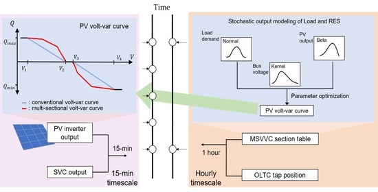
  • A new multi-sectional volt–var curve (MSVVC) of the PV inverter which follows the IEEE 1547 standard [10] is proposed. The MSVVC section table is updated by the main controller in the hourly timescale for the objective of network expected energy loss minimization, and the inverters operate along the MSVVC in the 15 min timescale.
  • To manage the uncertainty of the load demand and the RES output, parameters of the MSVVC were determined using the Monte Carlo-based stochastic analysis and non-linear optimization.
  • Using the active control of reactive power output in PV inverters, other reactive power compensators (i.e., SVCs) can obtain an operational margin. The proposed method can cope with more severe voltage issues than the conventional method.
  • The proposed method helps the RES inverter generate or absorb more reactive power than the conventional method, which, in turn, leads to network voltage profile improvement. Thus, the bus voltage in the distribution network can be kept within the allowed margin, even when the load demand and RES power outputs fluctuate.
The rest of this paper is organized as follows: Section 2 introduces the analysis methodology consisting of stochastic modeling, the proposed method, MSVVC, and the volt–var control framework. Section 3 presents a scenario construction that uses Monte Carlo sampling to demonstrate the effects of MSVVC. The test was implemented in the IEEE 33-bus system with several volt–var control devices, and Section 4 concludes the paper.

2. Proposed Methodology

2.1. Stochastic Modeling of Load Demand and RES Generation

The stochastic variation of load demand and RES generation follow normal and beta distributions, respectively [25,26,27]. Equation (1) shows the normal distribution function:
f ( x ) = 1 σ 2 π e x p [ 1 2 ( x μ σ 2 ) ]
where μ and σ denote the mean value and standard deviation, respectively:
f ( x ) = x α 1 ( 1 x ) β 1 B ( α , β )
Equation (2) shows the beta distribution function, which has two hyper-parameters, α and β . The mean value and variance are defined by the relationship between α and β as follows [27]:
M e a n : E [ X ] = α α + β
V a r i a n c e : σ 2 = α β ( α + β ) 2 ( α + β + 1 )
The probability density functions (PDFs) of the normal and beta distributions are illustrated in Figure 2. In this study, the stochastic variations in load demand follow the actual data that form the normal distribution; variations in PV output are based on the beta distribution [28,29].

2.2. Proposed Multi-Sectional Volt–Var Curve of PV Inverter

In Figure 3, the green curve shows the conventional VVC of the PV inverter recommended by the IEEE 1547 standard [10]. The conventional VVC can regulate the bus voltage through the linear relationship between the reactive power output and the voltage at the PCC, whereas the proposed MSVVC divides the VVC into multiple sections to actively compensate for reactive power. Although the PV inverter with conventional VVC can compensate reactive power according to the bus voltage, the objective function cannot be considered. Note that both conventional VVC and MSVVC have the same reactive power output limits.
To determine the optimal parameter of the MSVVC section table, the total expected energy loss has to be minimized while satisfying the rated voltage range over the variation of load demand and PV generation. For the entire system, Kirchhoff’s current law (KCL)-based power flow was performed as described in (5). The mathematical model can be formulated as shown in (5)–(13). The minimum/maximum vectors are denoted by a bar above/bar below (e.g., ( ̲ ) / ( ¯ ) ):
I b u s = Y b u s V b u s
m i n t j = 1 B r P l o s s j ( t )
subject to:
P l o s s j = I j 2 R j , j
V 0 ( t ) = V s u b + n t a p ( t ) × V t a p
n ̲ t a p n t a p ( t ) n ¯ t a p
Q ̲ S V C i Q S V C i ( t ) Q ¯ S V C i , i
Q ̲ P V i Q P V i ( t ) Q ¯ P V i , i
Q ̲ P V i = S P V i 2 [ P P V i ( t ) ] 2
Q ¯ P V i = S P V i 2 [ P P V i ( t ) ] 2
V ̲ i V i ( t ) V ¯ i , i
where B r denotes the total number of lines and (6) is the objective function, which is minimizing the power loss of the whole network. The power loss for branch j is as shown in (7). P l o s s j ( t ) represents the power loss of the j-th branch during a 15 min interval (t-th time) in an hour. V s u b is the primary voltage of the substation, which is typically 1.0 p.u. The secondary side voltage of the substation V 0 ( t ) can be calculated by (8), where V t a p is the voltage step per tap and n t a p denotes the tap position of the OLTC. In (9)–(11), the operation constraints of the volt–var control devices are shown; n t a p ( t ) is the OLTC tap position, Q S V C i ( t ) and Q P V i ( t ) denote the reactive power output of SVC and PV. The reactive power output limit of PV is estimated by (12) and (13), where the rated capacity and active power of the PV are represented by S P V i and P P V i ( t ) , respectively. In (14), the desired voltage limits are imposed for each node.
The decision variables in (6) are the points on the y axis of the proposed MSVVC section table. The points on the x axis are determined based on the probability distribution of the voltage with the PV installed:
P [ V p 1 L V V p 1 H ] = p 1
P [ V p 2 L V V p 2 H ] = p 2
where the values p 1 and p 2 determine the x coordinate voltages V p 1 L , V p 1 H , V p 2 L , and V p 2 H , respectively. In Figure 4, f ( V ) means kernel density estimation function, which is the distribution of bus voltages. Owing to the variations of load demand and PV generation, bus voltages also have a distribution function. The voltage V m is the mode value of the kernel density function, so it has a maximum probability. Therefore, the MSVVC on the inverter can include up to five points compared to the conventional VVC, as illustrated in Figure 4. If the x axis coordinate value exists in the dead band (voltage between V 2 and V 3 ), the y axis coordinate value is ignored.
As illustrated in Figure 5, for all x axis values determined by (15) and (16), the corresponding y axis values are determined by the proposed optimization process as Q p 1 L , Q p 1 H , Q p 2 L , Q p 2 H , and Q m . To inject or absorb more reactive power in proportion to the PCC voltage variation, the constraints between the y axis values are expressed as (17).
Q m a x Q p 1 L Q p 2 L Q m Q p 2 H Q p 1 H Q m i n , 0 Q m a x Q ¯ P V , Q ̲ P V Q m i n 0
Q M S V V C ( V ) = Q m a x if V V 1 Q M S V V C ( V 1 ) Q M S V V C ( V p 1 L ) V 1 V p 1 L ( V V p 1 L ) + Q p 1 L if V 1 V V p 1 L Q M S V V C ( V p 1 L ) Q M S V V C ( V p 2 L ) V p 1 L V p 2 L ( V V p 2 L ) + Q p 2 L if V p 1 L V V p 2 L Q M S V V C ( V p 2 L ) Q M S V V C ( V m ) V p 2 L V m ( V V m ) + Q m if V p 2 L V V m Q M S V V C ( V m ) Q M S V V C ( V p 2 H ) V m V p 2 H ( V V p 2 H ) + Q p 2 H if V m V V p 2 H Q M S V V C ( V p 2 H ) Q M S V V C ( V p 1 H ) V p 2 H V p 1 H ( V V p 1 H ) + Q p 1 H if V p 2 H V V p 1 H Q M S V V C ( V p 1 H ) Q M S V V C ( V 2 ) V p 1 H V 2 ( V V 2 ) if V p 1 H V V 2 0 if V 2 V V 3 Q M S V V C ( V 3 ) Q M S V V C ( V 4 ) V 3 V 4 ( V V 4 ) + Q m i n if V 3 V V 4
Equation (18) shows the formulation of the proposed MSVVC according to the x and y axis values. In (18), each section has the function of different slopes, which depends on the x axis and y axis values. Note that the function of all the sections is a linear function. In addition, if the selected voltage value exists in the dead band (i.e., between V 2 and V 3 ), there is no reactive power compensation.

2.3. Volt–Var Control Framework with Multi-Sectional Volt–Var Curve

Figure 6 illustrates the coordinated volt–var control framework in the hourly and 15 min timescale. In the hourly timescale, mechanical volt–var control devices such as OLTCs and CBs operate to regulate the slow voltage variation, and the optimal parameters in MSVVC section tables (illustrated as ‘Box’ in Figure 6) are determined by proposed optimization process. In the 15 min timescale, each PV inverter regulates the reactive power output according to the MSVVC. Moreover, SVCs absorb or inject reactive power based on the voltage set point. The proposed optimization sequences are as follows:
  • Stochastic modeling of load demand and PV output considering the uncertainty and intermittency nature is applied. The load demand and PV output follow normal and beta distribution, respectively.
  • Through the load flow analysis for the load demand and PV output data, voltage distribution is generated and fitted through kernel density function as presented in Figure 4.
  • The x-coordinate values of MSVVC (i.e., V p 1 L , V p 1 H , V p 2 L , V p 2 H , and V m ) are determined. To determine the x axis values, PV inverters do not compensate reactive power. They are defined by the probability p 1 and p 2 as shown in Equations (15) and (16). Moreover, the voltage with the maximum probability is defined to the mode value V m .
  • Through the proposed optimization process, the y coordinate values of MSVVC (i.e., reactive power output of PV inverter) are determined. The objective function is to minimize the total expected energy loss with following the several constraints as described in Equations (9)–(14). Through a series of processes, the MSVVC section table is generated every hour.
  • The DMS generates the MSVVC section table and regulates OLTC tap position every hour. Then, PV inverters compensate reactive power with MSVVC in the 15 min timescale. Moreover, SVCs compensate reactive power to maintain PCC voltages as 1.0 p.u.

3. Case Studies

3.1. Stochastic Model

Section 3.1 describes the stochastic model of load demand and RES generation. The 15 min intervals of the load demand and RES generation daily output profiles are shown in Figure 7. The load demand and PV output data are obtained from the transmission system operator of Korea (called Korea Power Exchange) [28]. The load data are derived from IEEE 33-bus system with constant power factor [30]. In this study, all DGUs are assumed to be solar PV.
The stochastic variations of RES generation are assumed to follow the beta distribution, where the shape parameters are set to α = β = 6.06 [29].
By considering the predicted load demand and RES generation with stochastic variations, 200 random scenarios were generated by Monte Carlo sampling for each time step (15 min), and load flow analysis was performed. Thus, 200 voltage combinations are generated for each 15 min timescale. Because MSVVC section tables are updated on an hourly timescale, a total of 800 sampling data are considered to determine the x axis values of MSVVC. The values of the x axis in the MSVVC depend on p 1 and p 2 . In this study, the probabilities p 1 and p 2 are set to 0.8 and 0.5, respectively. In other words, the probability of voltage existing between V p 1 L and V p 1 H is 80%, and the probability of voltage existing between V p 2 L and V p 2 H is 50% based on the mode voltage V m . The voltages V 1 , V 2 , V 3 , and V 4 are set to 0.92, 0.99, 1.01 and 1.08, respectively.

3.2. Parameter Settings

The IEEE 33-bus test system was used to verify the effectiveness of the proposed method, as shown in Figure 8. In this study, the primary voltage of the substation is set to 1.0 p.u., and the OLTC located at the substation has 20 taps with voltage variations of 0.005 p.u. per tap. Therefore, the OLTC voltage range was set to ±5%.
Table 1 shows the installed location and capacity information of PV inverters and SVCs. The rated capacity of all PV inverters are set to 824 KVA, and the maximum active power capacity is set to 700 KW according to Figure 9 [10].
The maximum output limit of the reactive power in the PV inverter is determined by the rated capacity and current active power output described in (12) and (13). The operating region is determined by the constraints shown in Figure 9. Moreover, the PV cannot exceed the maximum active power generation, nor can it absorb active power.
To solve the proposed non-linear optimization problem and efficiently simulate distribution systems with VVC, a co-simulation between two different software packages (OpenDSS 8.6.7.1 and MATLAB R2020b) is proposed. An overview of the co-simulation schemes is presented in Figure 10. The network topology is modeled and the load flow analysis is performed using OpenDSS, which is mainly used for distribution system analysis. Using the results of the load flow analysis (voltage, current, and power), the optimization problem was formulated and solved in MATLAB. In this study, a metaheuristic solver genetic algorithm is proposed to solve the problem.
A genetic algorithm is a metaheuristic method which imitates the natural selection process. The population pool is made up with several individuals and they are selected for the next generation by a fitness evaluation for each generation. Each selected individual called parents in a population pool has better properties. The individuals are defined as reactive power outputs of PV inverters and 10 PV plants are installed in this paper. Therefore, a maximum of 50 individuals became variables for one generation. Figure 11 shows the flowchart of the proposed genetic algorithm. The first step is to generate a population pool satisfying constraint (17) and set g e n = 1 . Then, the volt–var curve of the PV inverter is changed because individuals are defined as reactive power outputs of the PV volt–var curve. Based on the reflected information, load flow calculation is performed through OpenDSS. If all operating constraints from (9)–(14) are satisfied, the fitness evaluation (i.e., energy loss) proceeds. In a parents selection step, the elitist strategy is performed to copy the elite genes from the highest fitness individuals for choosing the next generation. In order to find the global optimal, the crossover and mutation processes are applied. In the crossover process, the operator selects two random individuals and exchanges their information. The mutation operator randomly changes one gene to give new information. The entire procedure is repeated until the maximum generation exceeded.

3.3. Simulation Results

In the proposed method, the DMS dispatches the optimal OLTC tap position every hour and transmits the MSVVC section table to each PV inverter. In the 15 min timescale, the reactive power output of the PV inverter is determined based on the MSVVC. If the active power output of the PV inverter is less than 5%, the reactive power cannot be compensated, as shown in Figure 9.
The DMS requests appropriate the tap changing of the OLTC to remain within the desired voltage range (±5% of the rated voltage). The 24 h OLTC tap position profile is shown in Figure 12. However, owing to the uncertainty of the load demand and RES output, the bus voltage can be violated during the OLTC tap dispatching time. To examine this, two case studies were conducted. In the first case (Figure 13a), the tap changing of the OLTC was performed based on the forecasted mean value of the load demand and RES power generation. In the second case (Figure 13b), the tap changing operation was coordinated with the MSVVC section table through the proposed method in Section 2.2. The bus voltage profiles produced by the 800 random scenarios are shown in Figure 13. The horizontal red lines in Figure 13 mean the voltage limits which are set to ±5% of the nominal voltages. Thus, above the horizontal red line are the upper limits of voltages (i.e., 1.05 p.u.) and below are the horizontal lower limits of voltages (i.e., 0.95 p.u.). Owing to the stochastic changes in load demand and RES output, the deterministic method violates the lower voltage limits, as illustrated in Figure 13a. However, the MSVVC meets the allowable voltage range and improves the voltage profile, as shown in Figure 13b.
The voltage performance index (VPI) is the root mean square deviation between the rated voltage V r a t e d i and bus voltage V k i . The VPI is applied to represent the voltage profile improvement. The rated bus voltage is defined as the mean value of the i-th bus and is affected by the current tap position and the output of other volt–var control devices. VPI is defined as follows:
V P I = i = 1 N B k = 1 N S ( V r a t e d i V k i ) 2
where N B is the number of buses in the system, and N S denotes the number of sampled data. Table 2 presents the comparison results of the different stochastic methods in terms of the average VPI and voltage violation. Three cases were performed to investigate the effect of MSVVC. In case 1, the tap positions are optimized to minimize the expected energy loss while satisfying the voltage limits with the conventional VVC. In case 2, the conventional VVC is used as in case 1, but the tap positions are equal to those of case 3. In case 3, the tap positions and MSVVC parameters are optimized to minimize the total expected energy loss while satisfying the rated voltage range.
In cases 1 and 3, the bus voltage range was satisfied within the allowed range. However, case 2 represents a low-voltage violation owing to the limited reactive power compensation capability of the conventional VVC. In addition, case 3 represents a minimum average VPI of 3.3086 compared to the other two cases.
Figure 14 describes the comparison of obtained MSVVC depending on the PV location at ninth hour. (PV7 means the PV is located in bus 7). Each PV inverter obtains a different VVC according to its location and time. Conventional VVC is represented by black lines for all PV inverters. However, all the MSVVC points are optimized to minimize the expected energy loss.
A comparison of the reactive power output in SVC at a specific time (hour = 9 h) is shown in Figure 15. Through the active control of the voltage regulation of the MSVVC, the reactive power output of the SVC can be saved through the proposed MSVVC. In bus 32, the reactive power output of the SVC is almost 100% of its capacity owing to the low voltage.
Table 3 compares the different cases in terms of expected energy loss and cumulative reactive power output of SVCs. Although case 1 shows better performance for the SVC margin among the cases, it shows poorer performance in terms of the expected energy loss. For case 3, the performance in terms of the expected energy loss is approximately 20.5% better compared to case 1. Moreover, case 3 has less expected energy loss and SVC output than case 2.

4. Discussion

In the proposed optimization process, the objective function in (6) and the voltage distribution under the Monte Carlo simulation ( V p 1 L , V p 1 H , V p 2 L , V p 2 H , and V m ) depend on the distribution network topology (line data and network configuration). Therefore, if the connection state between feeders is changed through network reconfiguration, the efficiency of the optimal parameter tuning of MSVVC in the previous time step could decrease. The system operator can observe the network topology status through DMS. Using this, in the proposed optimization process, the operator can use the data on the network topology changed in the previous time step to dispatch the optimal OLTC tap position and parameter of MSVVC in the next time step. The best way is to develop a strategy for network reconfiguration in the DMS separately and calculate the optimal parameter of MSVVC and the tap position of the OLTC coordinating with the expected network topology in the next time step. However, this is an area that will not be considered in this study.

5. Conclusions

This study proposed a new stochastic analysis-based VVC scheme for a smart inverter by dividing the curve into multiple sections. Compared to the conventional VVC, the proposed method offers multiple benefits such as reducing the total expected energy loss, obtaining the SVC output margin, improving the voltage profile, and mitigating voltage problems based on the variability of the RES power output. To analyze the uncertainty and intermittent nature of RES generation, the stochastic modeling of RES generation is adapted, which is also applied to the modeling of load demand. Owing to the differences in the characteristics of the devices, a coordinated dispatch strategy is proposed as two timescales. The OLTC tap position and MSVVC section table are scheduled in the hourly timescale. In the 15 min timescale, the PV inverter that follows the MSVVC, and the SVC outputs are dispatched. The proposed method is simulated by the collaboration of OpenDSS and MATLAB; OpenDSS models the distribution network and performs the power flow, and MATLAB solves the non-linear problem using a genetic algorithm to obtain VVC parameters.
The proposed method applies each PV inverter to minimize the total expected energy loss. The load demand and PV output were modeled based on historical data, and Monte Carlo sampling was applied to analyze its variations. In our future work, the application of MSVVC to maximize the hosting capacity in distribution networks will be investigated.

Author Contributions

The main idea was proposed by D.L., C.H. and G.J. The operating strategy and optimization algorithm were proposed by D.L. and C.H. The experimental results were collected and analyzed by D.L. All authors have read and agreed to the published version of the manuscript.

Funding

This work was supported by Korea Institute of Energy Technology Evaluation and Planning (KETEP) grant funded by the Korea government (MOTIE) (No. 20191210301890) and the National Research Foundation of Korea through the Framework of the International Cooperation Program, under Grant (2017K1A4A3013579).

Institutional Review Board Statement

Not applicable.

Informed Consent Statement

Not applicable.

Data Availability Statement

Data sharing not applicable.

Conflicts of Interest

The authors declare no conflict of interest.

References

  1. Sewdien, V.; Chatterjee, R.; Escudero, M.V.; Van Putten, J. System Operational Challenges from the Energy Transition. Cigre Sci. Eng. 2020, 17, 5–19. [Google Scholar]
  2. Moon, W.S.; Hur, J.; Kim, J. A Protection of interconnection transformer for DG in Korea distribution power system. In Proceedings of the 2012 IEEE Power and Energy Society General Meeting, San Diego, CA, USA, 22–26 July 2012; pp. 1–5. [Google Scholar] [CrossRef]
  3. Yun, S.Y.; Hwang, P.I.; Moon, S.I.; Kwon, S.C.; Song, I.K.; Choi, J.H. Development and Field Test of Voltage VAR Optimization in the Korean Smart Distribution Management System. Energies 2014, 7, 643–669. [Google Scholar] [CrossRef]
  4. Hwang, P.; Jeong, M.; Moon, S.; Song, I. Volt/Var optimization of the Korean smart distribution management system. In Proceedings of the 22nd International Conference and Exhibition on Electricity Distribution (CIRED 2013), Stockholm, Sweden, 10–13 June 2013; pp. 1–4. [Google Scholar] [CrossRef] [Green Version]
  5. Reno, M.J.; Broderick, R.J. Statistical analysis of feeder and locational PV hosting capacity for 216 feeders. In Proceedings of the 2016 IEEE Power and Energy Society General Meeting (PESGM), Boston, MA, USA, 17–21 July 2016; pp. 1–5. [Google Scholar] [CrossRef]
  6. Abbey, C.; Baitch, A.; Bak-Jensen, B.; Carter, C.; Celli, G.; El Bakari, K.; Fan, M.; Georgilakis, P.; Hearne, T.; Ochoa, L.N.; et al. Planning and Optimization Methods for Active Distribution Systems; International Council on Large Electric Systems (CIGRE): Paris, France, 2014. [Google Scholar]
  7. Resener, M.; Rebennack, S.; Pardalos, P.; Haffner, S. Handbook of Optimization in Electric Power Distribution Systems; Springer International Publishing: Berlin/Heidelberg, Germany, 2020. [Google Scholar] [CrossRef]
  8. Ustun, T.S.; Hashimoto, J.; Otani, K. Impact of Smart Inverters on Feeder Hosting Capacity of Distribution Networks. IEEE Access 2019, 7, 163526–163536. [Google Scholar] [CrossRef]
  9. Hatziargyriou, N.; Milanović, J.; Rahmann, C.; Ajjarapu, V.; Cañizares, C.; Erlich, I.; Hill, D.; Hiskens, I.; Kamwa, I.; Pal, B.; et al. Stability Definitions and Characterization of Dynamic Behavior in Systems with High Penetration of Power Electronic Interfaced Technologies; IEEE: Piscataway Township, NJ, USA, 2020. [Google Scholar]
  10. IEEE Standard for Interconnection and Interoperability of Distributed Energy Resources with Associated Electric Power Systems Interfaces; IEEE Std 1547–2018 (Revis. IEEE Std 1547–2003); IEEE: Piscataway Township, NJ, USA, 2018; pp. 1–138. [CrossRef]
  11. Bründlinger, R. Review and Assessment of Latest Grid Code Developments in Europe and Selected International Markets with Respect to High Penetration PV. In Proceedings of the 6th Solar Integration Workshop, Vienna, Austria, 15–17 November 2016. [Google Scholar]
  12. Italian Standard; CEI. CEI 0–16. In Reference Technical Rules for the Connection of Active and Passive Consumers to the HV and MV Electrical Networks of Distribution Company; CEI: Milano, Italy, 2008. [Google Scholar]
  13. Italian Standard; CEI. CEI 0–21. In Reference Technical Rules for Connecting Users to the Active and Passive LV Distribution Companies of Electricity; CEI: Milano, Italy, 2011. [Google Scholar]
  14. Antoniadou-Plytaria, K.E.; Kouveliotis-Lysikatos, I.N.; Georgilakis, P.S.; Hatziargyriou, N.D. Distributed and Decentralized Voltage Control of Smart Distribution Networks: Models, Methods, and Future Research. IEEE Trans. Smart Grid 2017, 8, 2999–3008. [Google Scholar] [CrossRef]
  15. Kekatos, V.; Zhang, L.; Giannakis, G.B.; Baldick, R. Voltage regulation algorithms for multiphase power distribution grids. IEEE Trans. Power Syst. 2015, 31, 3913–3923. [Google Scholar] [CrossRef] [Green Version]
  16. Ghosh, S.; Rahman, S.; Pipattanasomporn, M. Distribution Voltage Regulation Through Active Power Curtailment with PV Inverters and Solar Generation Forecasts. IEEE Trans. Sustain. Energy 2017, 8, 13–22. [Google Scholar] [CrossRef]
  17. Zhu, H.; Liu, H.J. Fast Local Voltage Control Under Limited Reactive Power: Optimality and Stability Analysis. IEEE Trans. Power Syst. 2016, 31, 3794–3803. [Google Scholar] [CrossRef]
  18. Maciejowski, J.; Goulart, P.; Kerrigan, E. Constrained Control Using Model Predictive Control. In Advanced Strategies in Control Systems with Input and Output Constraints; Springer: Berlin/Heidelberg, Germany, 2007; pp. 273–291. [Google Scholar] [CrossRef]
  19. Qin, S.; Badgwell, T.A. A survey of industrial model predictive control technology. Control Eng. Pract. 2003, 11, 733–764. [Google Scholar] [CrossRef]
  20. Bidgoli, H.S.; Van Cutsem, T. Combined local and centralized voltage control in active distribution networks. IEEE Trans. Power Syst. 2017, 33, 1374–1384. [Google Scholar] [CrossRef] [Green Version]
  21. Takasawa, Y.; Akagi, S.; Yoshizawa, S.; Ishii, H.; Hayashi, Y. Effectiveness of updating the parameters of the Volt-VAR control depending on the PV penetration rate and weather conditions. In Proceedings of the 2017 IEEE Innovative Smart Grid Technologies-Asia (ISGT-Asia), Auckland, New Zealand, 4–7 December 2017; pp. 1–5. [Google Scholar]
  22. Dao, V.T.; Ishii, H.; Hayashi, Y. Optimal parameters of volt-var functions for photovoltaic smart inverters in distribution networks. IEEJ Trans. Electr. Electron. Eng. 2019, 14, 75–84. [Google Scholar] [CrossRef] [Green Version]
  23. Rylander, M.; Reno, M.J.; Quiroz, J.E.; Ding, F.; Li, H.; Broderick, R.J.; Mather, B.; Smith, J. Methods to determine recommended feeder-wide advanced inverter settings for improving distribution system performance. In Proceedings of the 2016 IEEE 43rd Photovoltaic Specialists Conference (PVSC), Portland, OR, USA, 5–10 June 2016; pp. 1393–1398. [Google Scholar] [CrossRef]
  24. Lee, H.J.; Yoon, K.H.; Shin, J.W.; Kim, J.C.; Cho, S.M. Optimal parameters of volt–var function in smart inverters for improving system performance. Energies 2020, 13, 2294. [Google Scholar] [CrossRef]
  25. Niknam, T.; Zare, M.; Aghaei, J. Scenario-based multiobjective volt/var control in distribution networks including renewable energy sources. IEEE Trans. Power Deliv. 2012, 27, 2004–2019. [Google Scholar] [CrossRef]
  26. Wang, Z.; Wang, J.; Chen, B.; Begovic, M.M.; He, Y. MPC-based voltage/var optimization for distribution circuits with distributed generators and exponential load models. IEEE Trans. Smart Grid 2014, 5, 2412–2420. [Google Scholar] [CrossRef]
  27. Fabbri, A.; Roman, T.G.; Abbad, J.R.; Quezada, V.M. Assessment of the cost associated with wind generation prediction errors in a liberalized electricity market. IEEE Trans. Power Syst. 2005, 20, 1440–1446. [Google Scholar] [CrossRef]
  28. Korea Power Exchange. Available online: http://kpx.or.kr (accessed on 6 November 2020).
  29. Xu, Y.; Dong, Z.Y.; Zhang, R.; Hill, D.J. Multi-timescale coordinated voltage/var control of high renewable-penetrated distribution systems. IEEE Trans. Power Syst. 2017, 32, 4398–4408. [Google Scholar] [CrossRef]
  30. Baran, M.E.; Wu, F.F. Network reconfiguration in distribution systems for loss reduction and load balancing. IEEE Power Eng. Rev. 1989, 9, 101–102. [Google Scholar] [CrossRef]
Figure 1. Classification of control schemes (a) local control; (b) centralized control; and (c) combined control.
Energies 14 02785 g001
Figure 2. (a) PDF of normal distribution function; (b) and PDF of beta distribution function.
Energies 14 02785 g002
Figure 3. Schematic diagram of the conventional volt–var curve and multi-sectional volt–var curve.
Energies 14 02785 g003
Figure 4. Determination of x values in multi-sectional volt–var curve.
Energies 14 02785 g004
Figure 5. Representation of multi-sectional volt–var curve.
Energies 14 02785 g005
Figure 6. Proposed framework of the coordinated volt–var control.
Energies 14 02785 g006
Figure 7. Daily profile of the (a) load demand; and (b) RES power generation output.
Energies 14 02785 g007
Figure 8. Modified IEEE 33 radial distribution system.
Energies 14 02785 g008
Figure 9. Reactive power capability of PV inverter.
Energies 14 02785 g009
Figure 10. Overview of OpenDSS and MATLAB co-simulation.
Energies 14 02785 g010
Figure 11. The flowchart of the proposed genetic algorithm.
Energies 14 02785 g011
Figure 12. OLTC tap position.
Energies 14 02785 g012
Figure 13. Voltage profiles for (a) conventional VVC method; and (b) MSVVC method.
Energies 14 02785 g013
Figure 14. Comparison of the conventional VVC and MSVVC.
Energies 14 02785 g014
Figure 15. Comparison of the SVC reactive power output.
Energies 14 02785 g015
Table 1. PV inverter and SVC capacity information.
PV InverterSVC
Location (Node)7, 9, 11, 13, 19, 21, 22, 25, 27, 306, 10, 26, 32
CapacityS (KVA)824±500
Maximum P (KW)700-
Table 2. Comparison between case studies for VPI and energy loss.
Case 1Case 2Case 3
MIN voltage (p.u.)0.95040.94460.9505
MAX voltage (p.u.)1.03831.03831.0381
Average VPI3.51563.46783.3086
Table 3. Comparison of the SVC reactive power output.
Case 1Case 2Case 3
Expected energy loss (KWh)99.03985.77482.175
Voltage violationNoYesNo
SVC output (KVarh)670.571001.4954.71
Publisher’s Note: MDPI stays neutral with regard to jurisdictional claims in published maps and institutional affiliations.

