Comparison of Machine Learning Methods in Electrical Tomography for Detecting Moisture in Building Walls

Abstract

This paper presents the results of research on the use of machine learning algorithms and electrical tomography in detecting humidity inside the walls of old buildings and structures. The object of research was a historical building in Wrocław, Poland, built in the first decade of the 19th century. Using the prototype of an electric tomograph of our own design, a number of voltage measurements were made on selected parts of the building. Many algorithmic methods have been preliminarily analyzed. Ultimately, the three models based on machine learning were selected: linear regression with SVM (support vector machine) learner, linear regression with least squares learner, and a multilayer perceptron neural network. The classical Gauss–Newton model was also used in the comparison. Both the experiments based on real measurements and simulation data showed a higher efficiency of machine learning methods than the Gauss–Newton method. The tomographic methods surpassed the point methods in measuring the dampness in the walls because they show a spatial image of the interior and not separate points of the examined cross-section. Research has shown that the selection of a machine learning model has a large impact on the quality of the results. Machine learning has a greater potential to create correct tomographic reconstructions than traditional mathematical methods. In this research, linear regression models performed slightly worse than neural networks.

1. Introduction

The presence of moisture inside brick walls and walls is a serious problem both from the point of view of the maintenance and reliability of buildings and the health of the people living in them. Old and historical buildings are particularly exposed to moisture. In buildings erected a hundred years ago, ineffective technologies were used to protect the foundations against moisture in the soil. In addition, the passage of years means that the existing security measures are subject to degradation. The situation could be improved by periodic renovations, but economic reasons are often the explanation for their abandonment. The consequences of such omissions include the destruction of historic buildings and structures as well as old buildings, which in terms of architecture and utility may still be an attractive place to live or work. Building materials used in the construction of historical buildings are almost always porous. Ceramic bricks are very susceptible to the phenomenon of capillary leakage. Capillary leakage is the primary mechanism by which moisture moves from the soil up the walls. Moisture in the walls of buildings destroys their physical formation, leading to the weakening of the structure. In extreme cases, this may result in a construction disaster. For this reason, water-soaked load-bearing walls are not only an economic problem, which reduces the market value of real estate, but also poses a potential threat to human life and health.

Scientific research confirms that faulty insulation of foundations may cause long-term dampness in the walls. This, in turn, contributes to the appearance of harmful fungi, microorganisms and mold [1,2]. Chemical compounds contained in the water are another negative factor influencing the destructive effect of moisture. Water that enters the foundations from the soil can contain carbonates, sulfates, nitrates and chlorides. The salt contained in the water is particularly unfavorable for walls. It accelerates both the physical erosion of plasters as well as causing stains and discoloration, which adversely affects the appearance of the facade.

Health hazards resulting from excessive moisture inside bricks and walls relate to the increased possibility of various types of allergies among people staying inside the building. It turns out that there is a correlation between the level of building moisture and the incidence of diseases such as conjunctivitis, asthma and rhinitis in humans. Taking into account the above-described problems resulting from excessive humidity of building walls, especially those defined as old or historical, they should be considered significant.

1.1. Methods for Identifying Moisture in Building Walls

Solving the problem of the presence of water in the walls requires a prior diagnosis that would enable the identification of damp areas. For this purpose, many methods are used, the classification of which are presented in

Table 1. Classification of methods for testing the moisture content in masonry walls [2,3].

Methods of Testing the Moisture Content in Masonry Walls
Destructive (Invasive) Methods		Non-Destructive (Non-Invasive) Indirect Methods
Direct Methods	Indirect Methods
gravimetric	carbide Karl Fisher chemical method electrical resistive	paper indicators gamma radiation scanning neutrons nuclear magnetic resonance infrared thermography optics and videography dielectrics microwaves electrical impedance tomography (EIT)

. All methods of testing moisture in masonry can be divided into destructive (invasive) and non-destructive (non-invasive).

The gravimetric method is considered to be the most accurate method of determining the water content in masonry. It is a destructive method that requires the removal of a fragment of the wall. The sample is placed in a laboratory dryer and heated at 105 °C until the mass of the sample is stabilized. Water content is calculated as the difference in mass of the masonry sample before and after drying. Other names for the gravimetric method are the thermogravimetric method or the drying oven method. The main disadvantage of this method is the need to collect samples, i.e., physical damage to the wall, which is unacceptable, especially in the case of buildings under the administrative protection of monuments.

Another group of invasive methods is indirect methods. In general, the use of these methods has the advantage compared to the gravimetric method that the sampled masonry can be smaller (carbide and Karl Fisher’s). However, the advantages end there. The electrical resistive method does not require taking samples but requires drilling holes in the wall to insert steel rods. It is very onerous and strongly interferes with the wall substance, which excludes this method as an alternative to historical buildings. There is always a trade off when it comes to destructive methods. On the one hand, we strive to minimize interference with changing the structure of the tested wall, which means minimizing the measurement points. On the other hand, in order to obtain the most precise measurement result, the number of measurement points should be maximized. This is another major disadvantage of this type of method.

Non-destructive (non-invasive) indirect methods do not require limiting the number of measuring points, which is their benefit. The disadvantage of these methods, however, is that they can only analyze the humidity of the walls in a qualitative and not a quantitative manner. In practice, this means that they cannot be used for precise (e.g., percentage) determinations of wall humidity. You can only check which areas are more and which are less humid.

The point manner of taking measurements, determined by the necessity to determine individual places of wall sampling or places where the probe is applied, is a general disadvantage of all destructive and non-destructive methods of wall moisture assessment. The non-destructive indirect methods do not limit the performance of multiple measurements at different points of the wall. However, none of the point methods give a complete picture of the interior of the tested object. The method by which a cross-sectional or even three-dimensional image of the distribution of moisture inside the wall can be obtained is tomography. The most recognizable is medical computed tomography (CT). However, in recent years, due to the significant acceleration of the pace of IT technology development, industrial tomography, also called process tomography, has been gaining importance. Electrical impedance tomography (EIT), which was used in the described research to identify moisture in the walls of a historic building, belongs to the group of electrical tomography methods. Another type of electrical tomography is electrical capacitance tomography (ECT) [4,5,6,7,8,9] and electrical resistivity tomography (ERT). ECT is typically used to detect air crystals or air bubbles in pipes, vessels or industrial reactors [4,7]. ERT, on the other hand, is used in the recognition of geological structures [10,11,12], e.g., in the detection of aquifers, aggregate, metal deposits, etc. [4,9,13]. In the case of ECT, the value of the electrical permittivity ε is determined [14,15,16], while EIT and ERT reconstruct the conductivity σ [1]. Apart from electrical tomography (EIT, ECT, ERT) and CT [17], there are many other types of it, which, due to the physical phenomenon used, can be divided into: magnetism [18,19,20], sound waves [21], electromagnetic waves, X-rays, visible light [22], etc.

This paper deals with EIT. Due to the physical properties of bricks and walls, EIT is the most suitable for identifying moisture out of all the types of tomographic methods. The main advantages of the EIT method over other known methods were listed in [3]. A very important advantage of tomographic methods is their automation and algorithmization. The key to obtaining high-quality reconstructive tomographic images is, apart from the appropriate equipment, the algorithm responsible for converting the measured values (inputs) into the output image. From a mathematical point of view, the task of the algorithm is to solve an inverse problem, which is also ill-posed [23]. Mathematical equations are rather poor at solving inverse and ill-posed problems, but machine learning algorithms, with iterative loops paralleled by fast CPUs and GPUs, have great potential. This is especially important on the eve of the 4th industrial revolution [24,25], when the world is entering the 5G era. In this respect, in-depth research on the use of EIT to detect moisture in the walls of buildings seems to be fully justified.

1.2. EIT Algorithmic Methods

From a mathematical point of view, the reconstruction of the electrical conductivity distribution in the EIT comes down to solving a nonlinear ill-posed inverse problem based on noisy data [26]. All the modalities used to solve the EIT inverse problems can be divided into two groups: direct and iterative methods. The direct methods, among others, include: Gauss–Newton with Tikhonov or Laplace regularization [1], Total Variation [3], Level Set [27], etc. Examples of iterative methods are: sparse Bayesian learning (SBL) [26,28,29], Least Absolute Shrinkage and Selection Operator (Lasso) [1], Linear Regression and Least-Angle Regression (LARS) [1], Elastic Net [1,3], Artificial Neural Networks (ANN) [1], Logistic Regression [30], etc.

In the above list, the SBL method deserves special attention. The authors of this method obtained significant performance improvement by imposing structure-aware priors on the learning process to incorporate the prior knowledge that practical conductivity distribution maps exhibit clustered sparsity and intra-cluster continuity. The SBL method not only achieved a high-resolution estimation and preserved the shape information even in low signal-to-noise ratio scenarios, but also avoided the time-consuming parameter tuning process. Successive, improved versions of the SBL method increased the efficiency of the algorithm and made it possible to obtain shorter reconstruction times.

1.3. Objective of Research and Novelties

The main contribution of the authors presented in these studies is the use of the original model structure for the reconstruction of tomographic images. The concepts of EIT algorithms based on machine learning, which combine linear regression with a support vector machine and linear regression with the least squares method, are presented.

A characteristic feature of the proposed solution is the use of multiple single-output machine trained models instead of a single model with a large number of outputs. In the case under study, the reverse problem is to transform 448 measurements into 7765 pixel values of the three-dimensional output image. The colors of the pixels reflect the conductivities of individual finite elements arranged on the mesh of the part of the wall being tested. Let $\mathcal{M}$ be the multi-output machine learning model, $\tilde{\mathcal{M}}$ the single-output machine learning model, $\left\{x_1,\dots ,x_{448}\right\}$ the vector of measurements, $\tilde{y}$ the singular pixel value, and $\left\{y_1,\dots ,y_{7765}\right\}$ be the set of all pixel values in the spatial tomographic image. The new approach can be described as $\left(\left\{x_1,\dots ,x_{448}\right\}\to \tilde{\mathcal{M}}\to \tilde{y}\right)\times 7756$ and the classical approach as $\left\{x_1,\dots ,x_{448}\right\}\to \mathcal{M}\to \left\{y_1,\dots ,y_{7765}\right\}$.

Another novelty is the use and quality assessment of machine learning models based on linear regression equipped with a support vector machine (SVM) and least square learners, compared to artificial neural networks (ANN) and the classic Gauss–Newton (GN) method.

1.4. Structure of the Paper

The paper consists of four chapters. The first section, the Introduction, contains a description of the problems related to dampness in buildings, a review of known methods of identifying moisture in walls, a description of the types of tomography and the authors’ own contribution. The second section, entitled Materials and Methods, describes the research object, which was the historical building. This section presents the results of the research used to validate the new EIT algorithms. In addition, the procedure for acquiring measurement data is described and the Gauss–Newton method and machine learning models used in the research are described. The third section includes research results obtained by using GN, linear regression and neural network algorithms. The Results section contains both reconstructions based on real measurements and on simulation data. Finally, the fourth section contains an overview and summary of the most important aspects of the research work carried out, the results obtained and the conclusions. It also includes information on future research.

2. Materials and Methods

This section describes the historical building as a research object. The tomographic hardware used and the ways of taking measurements are also included. The last part of this section presents the methodological basis of the statistical and machine learning methods used to solve the inverse problem in electrical tomography.

Our earlier publications ([1] (Section 2.1) and [31]) describe in detail both the EIT tomograph and the electrodes used in this research. The measurements were made using the Polar GND EIT method, at 1 kHz frequency and 100 uA excitation current. By means of a multiplexer, the tomographic system generates 448 values of voltage drops between individual electrode pairs in short time intervals. These are the input data for the EIT system. The electrode consists of three modules: a special electrode, a printed circuit board (PCB) with a socket and a mounting system. Mechanically, the modules are connected to each other by means of two sleeves placed one inside the other. Before separation, they are secured by a collar placed on the upper sleeve. The PCB is made of double-sided 1.54 mm thick laminate with an SMB1251B1-3GT30G-50 socket. Both pictures of the tomograph and electrodes can be found in [1].

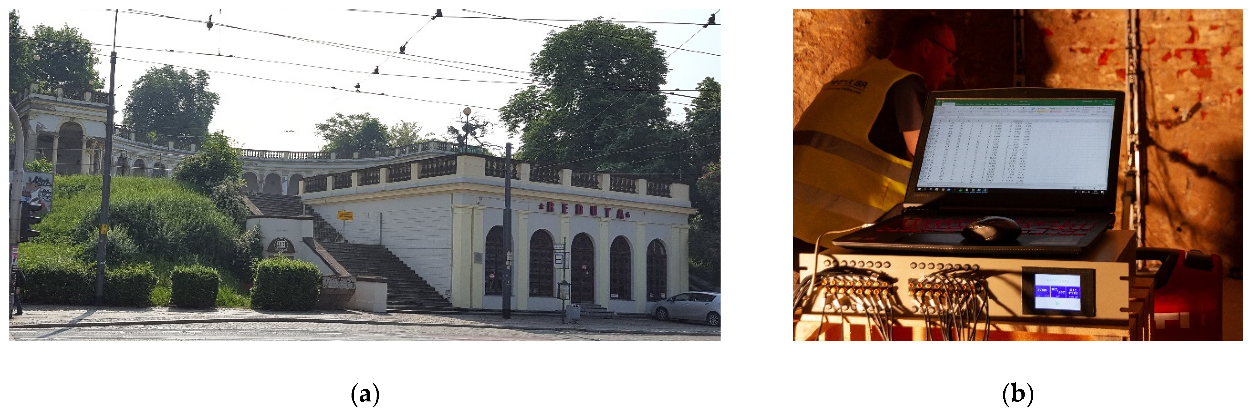
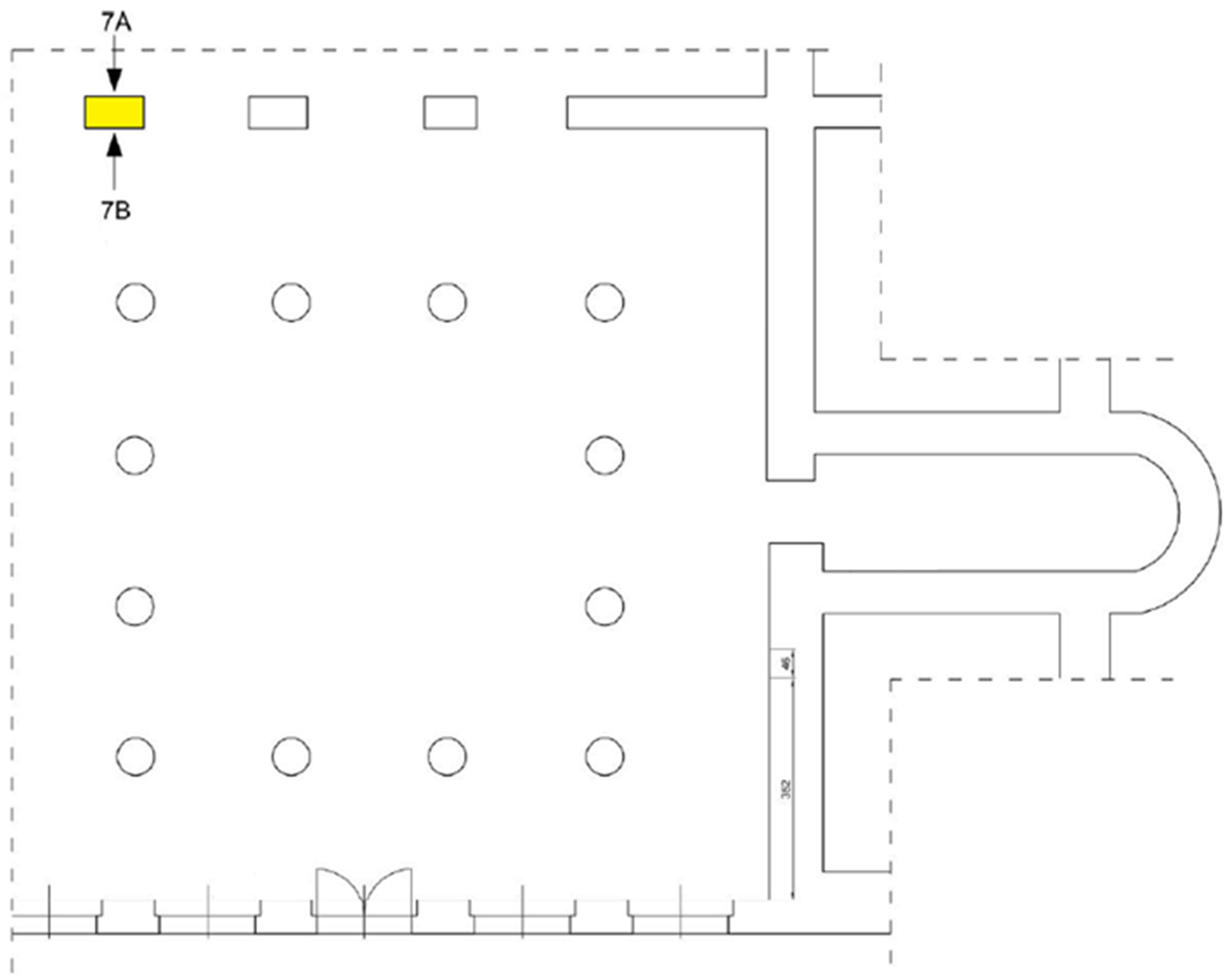
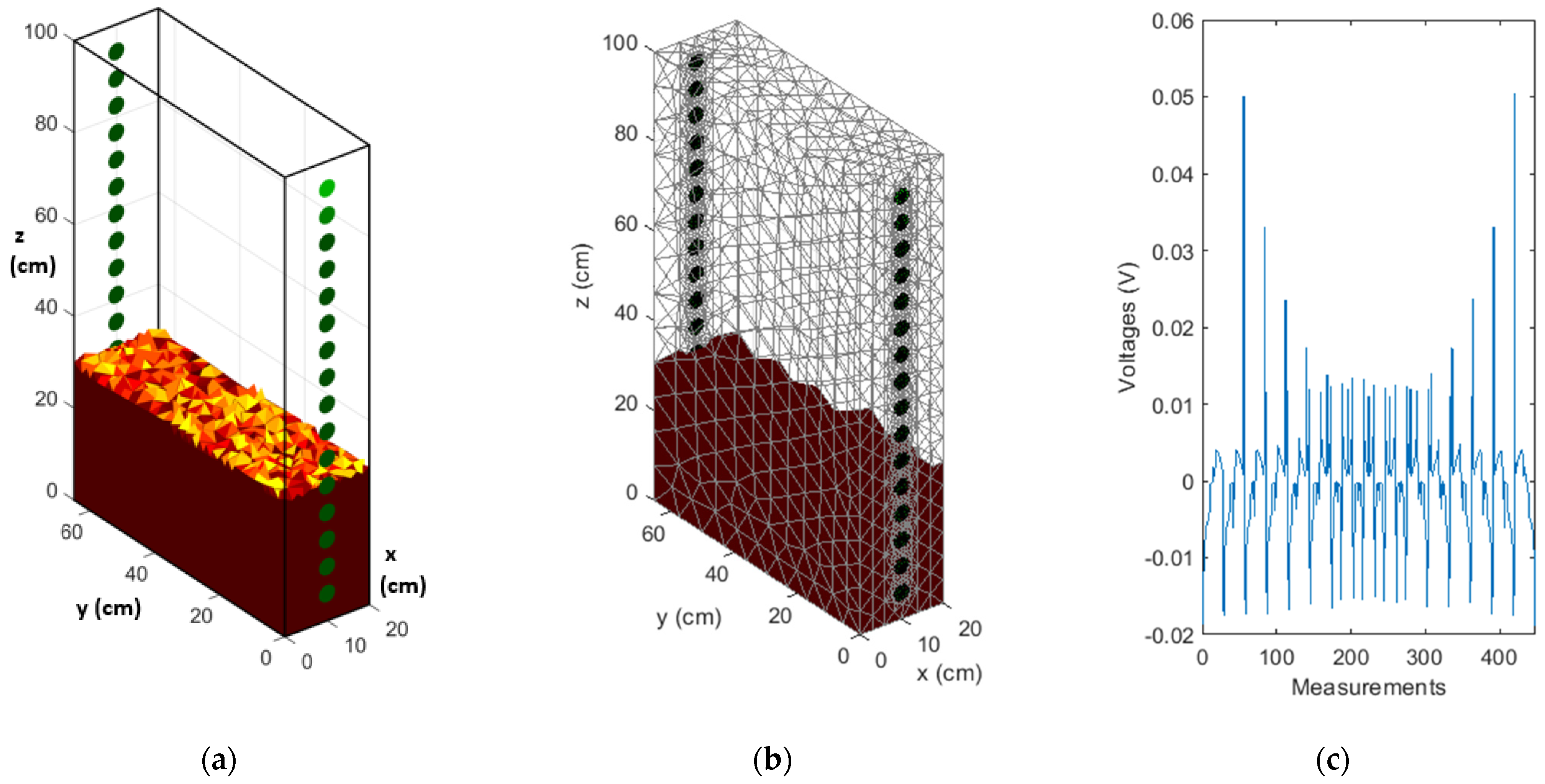
2.1. Historical Building as a Research Object

The research was carried out inside the Bastion Sakwowy (German: Taschenbastion) located on Sakwowy Hill in Wrocław (Poland) [3]. The bastion is a remnant of the former city fortification system of the city of Wrocław, on whose site, after demolishing the walls on the order of the French invaders in 1807, the recreational Sakwowy Hill was created. The hill, after the of building a belvedere and a tower on it in 1867, was renamed Liebichs Höhe (Liebich’s hill). The Bastion Sakwowy mainly has walls made of solid ceramic bricks on a lime mortar, 50–90 cm thick. The walls are in fairly good condition but they are very damp, and are covered with salt efflorescence and mold fungi. One of the tasks that will be carried out as part of the renovation works will be an attempt to dry the building. For this purpose, it is necessary to determine the degree of moisture in its walls.

Figure 1a shows the facade of the Peristyle Pavilion inside which the research was conducted. Figure 1b shows the test stand with a tomograph, laptop and electrodes placed against the wall, visible in the background.

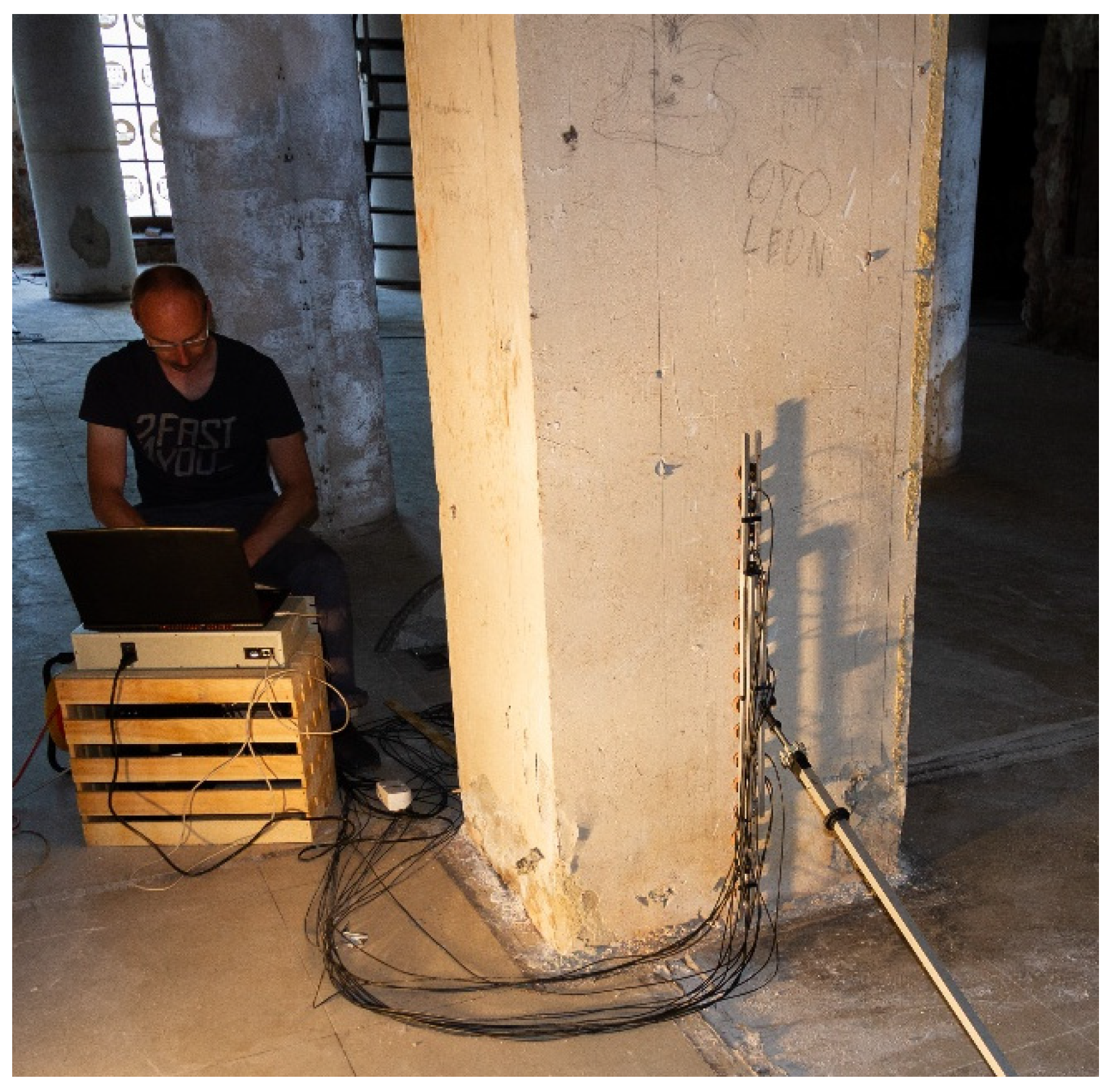
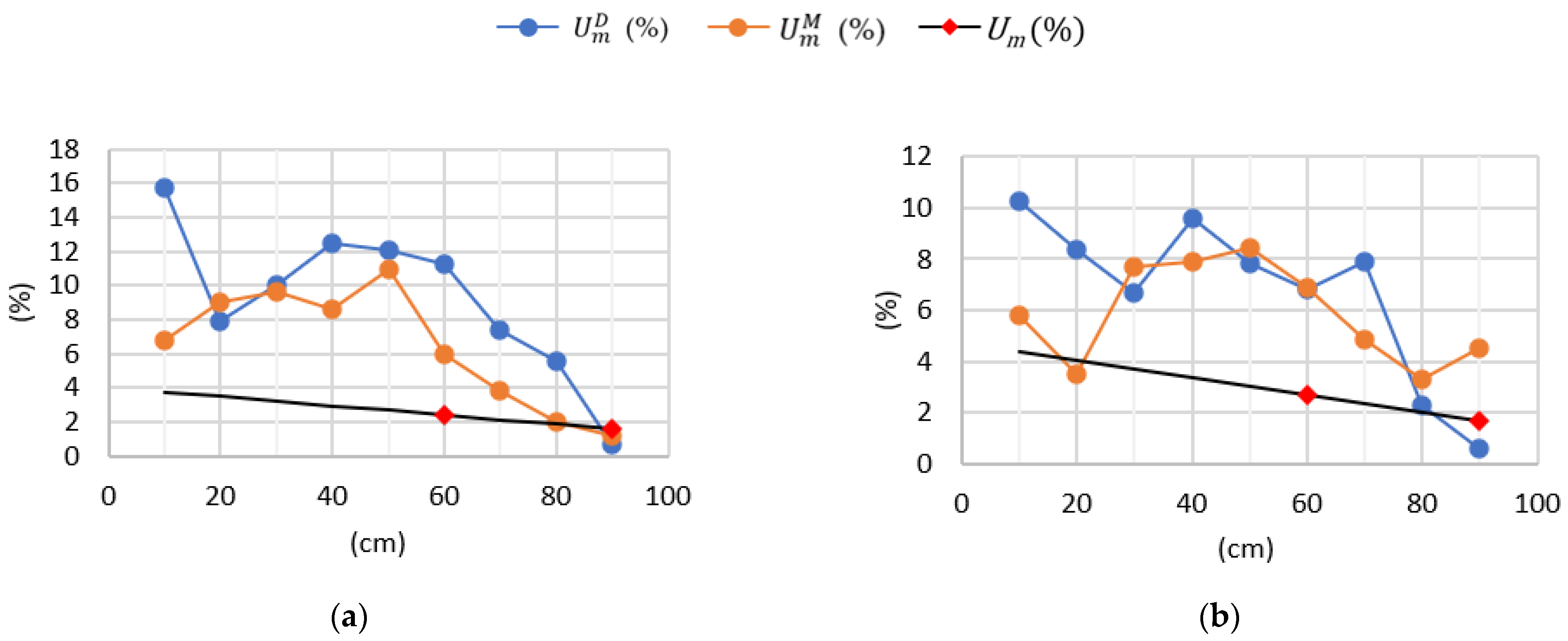
2.2. Validation Measurements

The inner pillar of the building was subjected to humidity tests to compare the effectiveness of selected machine learning algorithms for EIT imaging tasks. In order to validate the methods based on electrical tomography, the same pillar was also tested using three traditional methods. Two of them were non-invasive and one was invasive. The first was the non-destructive dielectric method using the GANN UNI 2 m (GANN Mess-u. Regeltechnik GmbH, Stuttgart, Germany) with the B50 ball probe. The research range of this meter is up to about 50 mm into the wall.

The second was the microwave method with the use of the T 600 m (TROTEC GmbH and Co. KG, Heinsberg, Germany) with a test range of up to about 300 mm into the wall. The third gravimetric method is invasive, but this approach is considered to be the most reliable method of testing the humidity of walls.

The gravimetric method uses a moisture analyzer which works according to the thermogravimetric principle, also known as the “Loss on Drying” principle. A moisture analyzer consists of two key components, a balance and a heater. To measure the moisture content, the initial weight of the sample is recorded, and then a heater (e.g., a halogen lamp) heats and dries the sample. During this time, the built-in balance records the sample weight on an ongoing basis. When the sample no longer loses weight, the instrument turns off and the moisture content is calculated. Total weight loss is used to calculate the moisture content.

Figure 2 shows a plan of the ground floor of the building which is the subject of the research. In the space where the wall humidity was measured, there were twelve round brick pillars and three rectangular pillars. In the upper left corner of the plan, a rectangular pillar is distinguished, which was subjected to the tests described in this paper. The arrows indicate the sides of the pillar on which the humidity measurements were carried out. 7A and 7B show vertical rails of 16 EIT electrodes each applied to the north and south sides of the internal pillar under test.

Pillars act as architectural supports. The intact internal structure of the pillar is a necessary condition to withstand high static loads. The degradation of the pillars caused by the water inside them may cause the floor and even the entire building to collapse. For this reason, there was a load-bearing pillar among the examined building elements.

Figure 3 shows the measuring stand. You can see the tested pillar with the EIT electrodes placed opposite each other, which correspond to the measurements marked with symbols 7B and 7A in Figure 2. Next to the pillar, on a wooden box, there is a tomograph and a laptop, in which machine learning algorithms convert the measurement data into images.

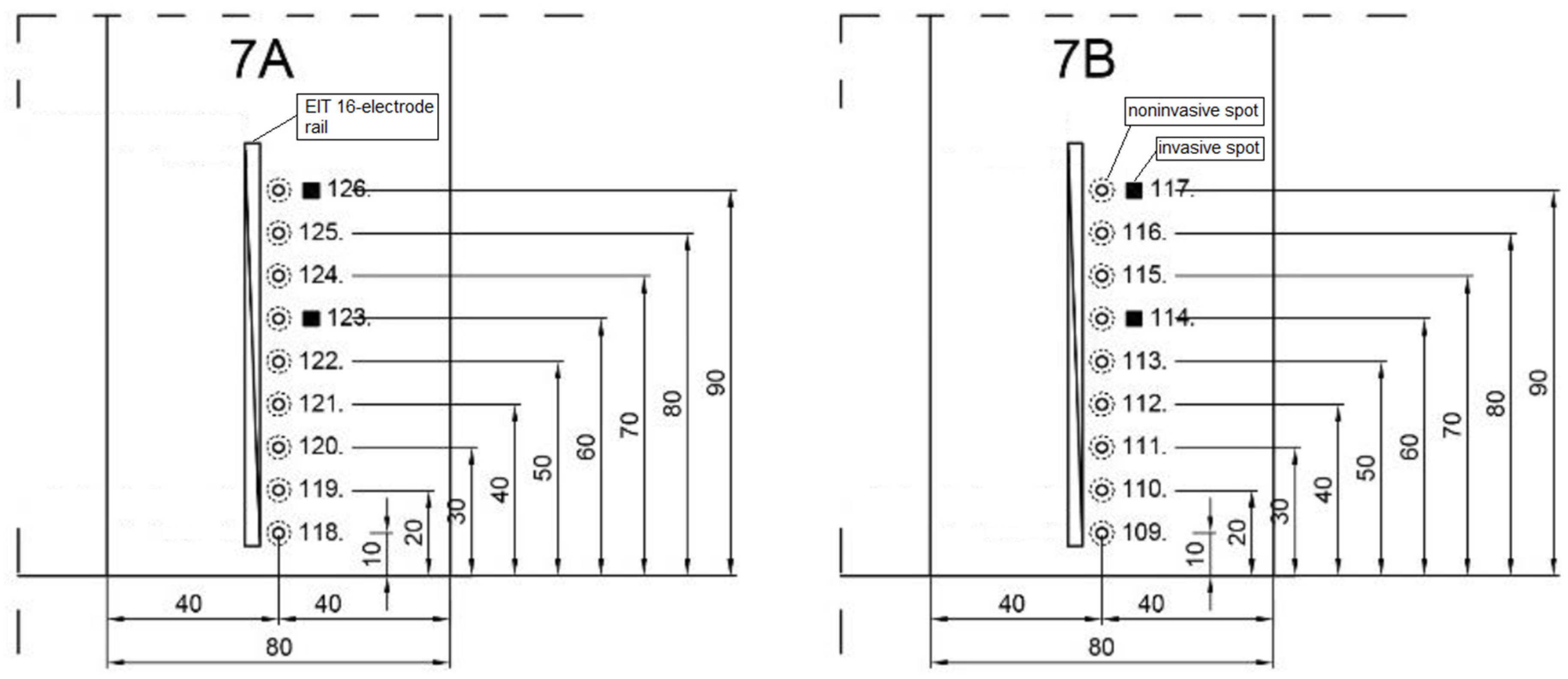
Figure 4 presents the arrangement of all measurement points on both sides of the tested pillar. Electrode application sites during non-invasive measurements (EIT, dielectric and microwave) are marked with the symbol “ ”. The sites for sampling the wall for invasive measurements using the gravimetric method are marked with the symbol “ ”. All distances are in millimeters.

As mentioned before, the dielectric and microwave techniques belong to the group of indirect methods. For this reason, these methods do not output the percent mass moisture $U_m$, but some unitless parameters $X_D$ and $X_M$. In the case of the dielectric method ($X_D$), the change of the dielectric constant of the tested material due to moisture is used. In turn, the microwave method ($X_M$) is based on the measurements of the attenuation of microwaves passing through the damp material. This means that in the case of both methods, the mass moisture $U_m$ is not measured directly during the test, but on another physical property of the material, the value of which depends on the amount of water contained in it. To determine the value of the mass moisture content $U_m$ it is necessary to determine the correlation relationship between the dimensionless parameter ($X_D$ or $X_M$) measured in a given method and the mass moisture content $U_m$.

It is not possible to obtain a correlation relationship for a single tested element in an object, in this case a pillar, because the number of measurement points is too small (9). Such a correlation relationship is determined in practice for the entire object, because the minimum number of validation measurements should be 30. Equation (1) presents experimentally established linear relationships for the building on the Partyzantów Hill that enables the determination of mass moisture $U_m$ based on dielectric and microwave measurements

$$U_m^D=0.1691·X_D-6.417$$

(1)

where $U_m^D$ is the mass moisture calculated on the basis of the dielectric parameter $X_D$. Similarly, Equation (2) shows the relationship between the mass moisture $U_m^M$ and the microwave parameter $X_M$.

$$U_m^M=0.3418·X_M-6.8071$$

(2)

The results of the validation measurements are presented in

Table 2. Results of validation measurements. Percentage mass humidity obtained by: dielectric $U_m^D$, microwave $U_m^M$, and gravimetric $U_m$ methods.

# of Spot	Side of the Wall	Distance of the Measuring Point to the Floor Level	Dielectric Meter Indication		Microwave Meter Indication		$\mathbf{Mass}\mathbf{Humidity}\mathbf{Determined}\mathbf{in}\mathbf{the}\mathbf{Laboratory}{\mathit{U}}_{\mathit{m}}(\%)$
			${\mathit{X}}_{\mathit{D}}$	${\mathit{U}}_{\mathit{m}}^{\mathit{D}}(\%)$	${\mathit{X}}_{\mathit{M}}$	${\mathit{U}}_{\mathit{m}}^{\mathit{M}}(\%)$
(1)	(2)	(3)	(4)	(5)	(6)	(7)	(8)
109	7B	10 cm	98.5	10.25	36.8	5.8	-
110		20 cm	87.3	8.3	30.1	3.5	-
111		30 cm	77.6	6.7	42.5	7.7	-
112		40 cm	94.8	9.6	43.0	7.9	-
113		50 cm	84.2	7.8	44.6	8.4	-
114		60 cm	78.1	6.8	40.0	6.9	2.70%
115		70 cm	84.6	7.9	34.1	4.8	-
116		80 cm	51.6	2.3	29.5	3.3	-
117		90 cm	41.2	0.6	33.2	4.5	1.70%
118	7A	10 cm	131.2	15. 8	39.9	6.8	-
119		20 cm	84.8	7.9	46.3	9.0	-
120		30 cm	97.5	10.1	48.1	9.6	-
121		40 cm	111.9	12.5	45.2	8.6	-
122		50 cm	109.6	12.1	52.0	11.0	-
123		60 cm	104.4	11.2	37.5	6.0	2.41%
124		70 cm	81.8	7.4	31.1	3.8	-
125		80 cm	70.6	5.5	25.7	2.0	-
126		90 cm	41.8	0.7	23.5	1.2	1.59%

. Column (1) contains the numbers of the measurement points in accordance with Figure 4. Column (2) contains the symbols of the sides of the tested pillar as shown in Figure 2 and Figure 4. Column (3) contains information on the distribution of the measurement points on the pillar surface. Columns (4) and (5) contain the results of dielectric measurements, while columns (6) and (7) contain the results of microwave measurements. Column (8) contains the results of measurements by the invasive gravimetric method.

Figure 5 envisions the results of validation measurements placed in Table 2. To facilitate the comparison of the results obtained with the three methods, dielectric, microwave and gravimetric, all the results are presented as percentage mass humidity $U_m$. In Figure 5, the horizontal axes indicate the distances of the measurement points from the ground level. The real measurements in Figure 5a,b are marked with thick dots. Despite the fluctuations of $U_m^D$ and $U_m^M$ in Figure 5, there is a visible trend of decreasing humidity with the increasing distance from the ground. The dynamics of decline are similar for $U_m^D$ in Figure 5a,b and $U_m^M$ in Figure 5a. The decrease in the humidity of $U_m^M$ in Figure 5b is less dynamic, but it may be the result of the non-uniform distribution of moisture inside the tested pillar.

The black lines show the decrease in humidity inside the pillar after two invasive measurements taken on both sides (7B and 7A). The real gravimetric measurements in the charts are marked with red diamonds. The black straight $U_m$ lines were determined by interpolation. The measurements for side 7B correspond to measurement spots #114 and #117, and for side 7A to spots #123 and #126 (see Table 2).

In order to supplement the validation of humidity tests, photos of the pillars were taken with a professional thermal imaging camera. The FLIR T540 (FLIR Systems, Inc., 27700 Southwest Parkway Avenue Wilsonville, OR 97070 USA) camera was used. Figure 6 shows photos of the pillars, among which there is also the research object. Considering that wet surfaces are cooler than dry surfaces due to evaporation, the pictures clearly show that the moisture in the pillars accumulates closer to the floor. It should be remembered that thermal images only erase the surfaces of the tested objects. Therefore, it is impossible to judge how the moisture is distributed inside the pillars based on the infrared photos.

2.3. Methods of Creating a Tomographic Image

This section describes the algorithmic methods that were used in these studies for EIT imaging. The authors’ intention was to compare machine learning methods with traditional methods, as well as to compare machine learning methods with each other. Due to the large number of different algorithmic approaches and techniques used in the EIT, it was not possible to cover them all in this study. Therefore, as part of the initial selection of methods, four classical methods, not belonging to the group of machine learning methods, and six methods based on typical machine learning were analyzed. As part of classical methods, the following were tested: Gauss–Newton with Tikhonov regularization, Gauss–Newton with Laplace regularization, Total Variation, and Level Set. The analyzed machine learning methods including Least-Angle Regression (LARS), Elastic Net, Artificial Neural Networks (ANN), Logistic Regression, Linear Regression with SVM learner (LR-SVM), and Linear Regression with least squares learner (LR-LS). The initial selection of methods was based on a simulation-generated set of training cases. The number of cases for each of the methods was 44,000.

In the case of 3D reconstruction, it is not possible to use real measurements to train models based on supervised learning. The reason for this is the lack of 3D reference images. Such reference images can be obtained in sufficiently large numbers only by using simulation generators. Ultimately, four methods were selected. One method among the classic methods and three machine learning methods. These four methods are described below.

Figure 7 shows the model of the multiple EIT system converting electrical signals into a 3D reconstruction image. This type of transforms the input measurements into built pixel-by-pixel tomographic images was used for all the methods tested in this research.

2.3.1. Gauss–Newton (GN)

Imaging algorithms based on Tikhonov regularization are popular, and are often taken as a benchmark [32]. For example, in [33], the standard Tikhonov regularization for EIT in unbounded domains was studied. In this research, the Gauss–Newton model with Tikhonov regularization was used. GN is an example of a non-machine learning EIT imaging method. The mathematical formula of the complete electrode model, currently the most accurate model, is presented below. With this model, an accuracy comparable to the experimental precision can be achieved and is, therefore, a suitable model for EIT applications. The complete electrode model uses non-standard boundary conditions to capture important features of the EIT experiments, e.g., the discrete nature of the electrodes, the contact impedance effect and the shunt effect. Suppose $\mathsf{\Omega }\in {ℝ}_{\ast }^L$ (d = 2, 3) is an open bounded domain with a Lipschitz boundary $\mathsf{\Gamma }$. ${\left\{e_l\right\}}_{l=1}^L\subset \mathsf{\Gamma }$ is a set of L electrodes, each with a positive surface measure. Suppose all electrodes are connected but disjointed from each other. The considered model can be represented as (3):

$$\left\{\begin{array}{c} -\nabla ·\left(\sigma \nabla u\right)=0 in \mathsf{\Omega } \\ u+z_l\sigma \frac{\partial u}{\partial n}=U_l on e_l, l=1,2,\dots ,L\\ \begin{array}{c} \underset{e_l}{\overset{}{{\displaystyle \int }}}\sigma \frac{\partial u}{\partial n}ds=I_l for l=1,2,\dots ,L \\ \sigma \frac{\partial u}{\partial n}=0 on \mathsf{\Gamma }\backslash \underset{l=1}{\overset{L}{{\displaystyle \cup }}}{e}_L \end{array}\end{array}\right.$$

(3)

where $x_i$ is the i-th $\sigma$ is electrical conductivity, $u$—electrical potential, $I\in {ℝ}_{\ast }^L$ is the input current, ${ℝ}_{\ast }^L=\left\{I\in {ℝ}_{}^L : {{\displaystyle \sum }}_{l=1}^L{I}_l=0\right\}$, $z_l$ is positive contact impedances, $\sigma \frac{\partial u}{\partial n}$ is a Neumann boundary condition operator.

The analysis of Tikhonov linearized models relies mainly on the boundedness of the derivative operator $F^{\prime }\left({\sigma }_0\right)$. In the case of nonlinear models, it uses the differentiability of the forward operator $F\left({\sigma }_0\right)$. Tikhonov regularization describes Equation (4)

$$F^{\prime }\left({\sigma }_0\right)\vartheta +F\left({\sigma }_0\right)-{\varphi }^{\delta }=0$$

(4)

where $F^{\prime }\left({\sigma }_0\right)$ is a bounded operator, ${\varphi }^{\delta }=F\left({\sigma }_0\right)+{\tilde{\varphi }}^{\delta }$ while ${\tilde{\varphi }}^{\delta }$ symbolizes the linearized noisy data, $\vartheta \in \mathcal{A}$ when $\mathcal{A}$ is an admissible set such as $\mathcal{A}=\left\{\sigma \in L_{\infty }\left(\mathsf{\Omega }\right)\right\}$ or $L_p\left(\mathsf{\Omega }\right)$ norm $\left(1\le p\le \infty \right)$.

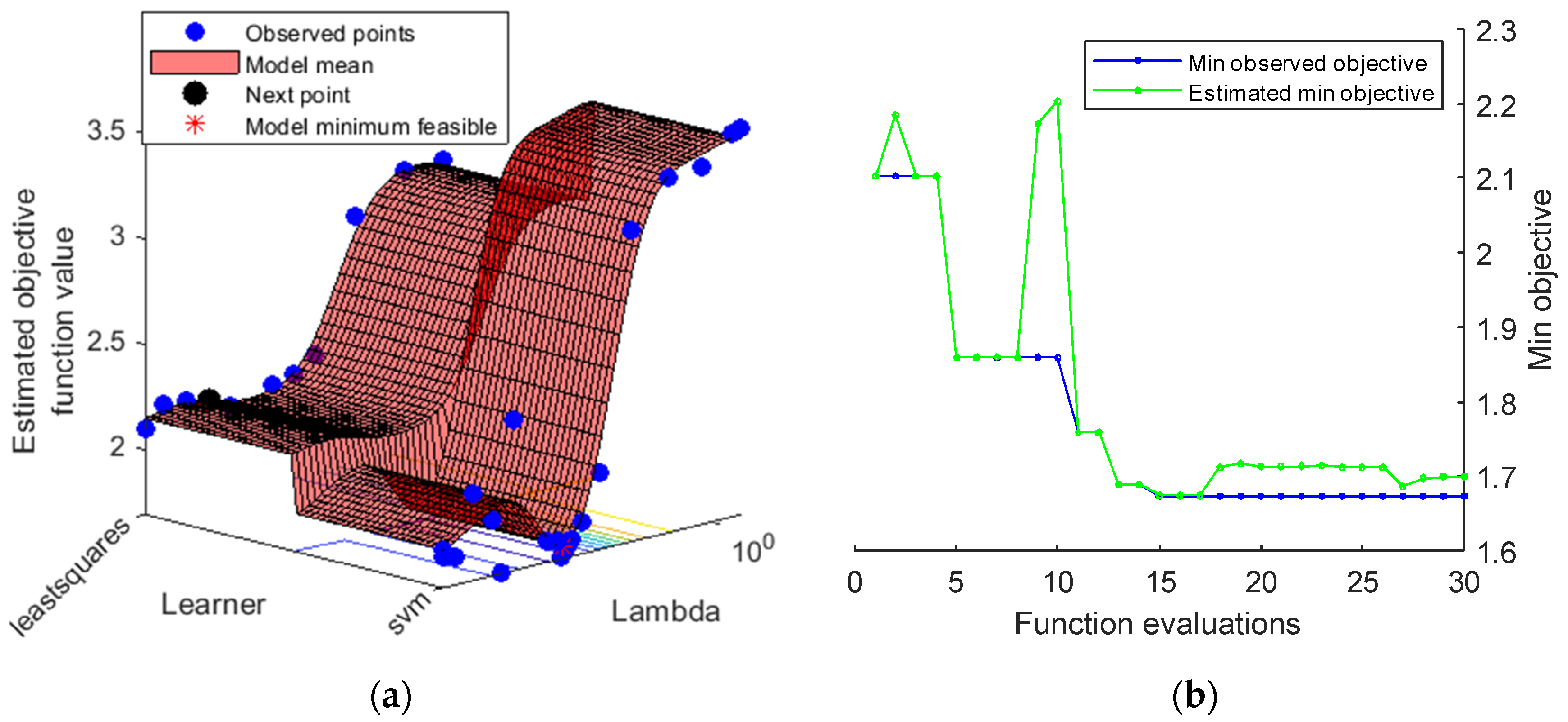
2.3.2. Linear Regression with SVM Learner (LR-SVM)

Linear regression (LR) via support vector machine (SVM) was used to reconstruct the tomographic images [34]. The algorithm was optimized for high-dimensional data. For this reason, a regression model that uses an L1 regularization technique called Lasso was used (Least Absolute Shrinkage and Selection Operator). Lasso adds the “absolute value of magnitude” of coefficient as a penalty component to the loss function. As a “Learner”, a linear regression model based on the SVM method was used [35]. The loss function for the linear regression model type was $f\left(x\right)=x\beta +b$, where $\beta$ is a vector of $p$ coefficients, $x$ is an observation from $p$ predictor variables, and $b$ is the scalar bias. In the implemented algorithm, the mean squared error (MSE) was calculated as a loss function and takes the form of the formula $𝓁\left[y,f\left(x\right)\right]=\max \left[0,\left|y-f\left(x\right)\right|-\epsilon \right]$ where $y\in \left(-\infty ,\infty \right)$ is the reconstructive response value. The Lasso cost function is described by the Equation (5)

$$\underset{{\beta }_0,\beta }{\min }\left(\frac{1}{2N}{\displaystyle \sum }_{i=1}^N{\left(y_i-b-x_i^T\beta \right)}^2+\lambda {\displaystyle \sum }_{j=1}^p\left|{\beta }_j\right|\right)$$

(5)

where $N$ is the number of observations. $x_i^T$ consists of data, a transposed vector of length $p$ at observation $i$. $y_i$ is the reconstruction at observation $i$. $\lambda$ is a non-negative regularization parameter corresponding to the Lambda. In this research Lambda =$1/N$. The parameters $b$ and $\beta$ are respectively a scalar bias and a vector of length $p$. As $\lambda$ increases, the number of non-zero $\beta$ components decreases.

Initial linear coefficient estimates $\beta$, specified as the comma-separated pair consisting of ‘Beta’ and a $p$-dimensional numeric vector or a $p\times L$ numeric matrix. $p$ is the number of predictor variables in $X$ and $L$ is the number of regularization-strength values. If a $p$-dimensional vector is specified, then the algorithm optimizes the objective function $L$ times by the following process. In the first step, the algorithm optimizes using $\beta$ as the initial value and the minimum value of Lambda ($\lambda$) as the regularization strength. In the second step, the software re-optimizes using the resulting score from the previous optimization as a warm start and the next lowest value in $\lambda$ as the regularization strength. Finally, the software repeats the second step until it exhausts all the values in Lambda. In this way, for a vector of non-negative values, the algorithm sequentially optimizes the objective function for each individual value in Lambda in ascending order. Each estimated coefficient of zero maintains its value when the software optimizes with successive values in Lambda. The model returns the coefficient estimates for all optimization iterations.

One of the key subsystems of the LR algorithm used is the objective function minimization technique. This technique is defined as a comma separated pair, consisting of a “Solver” and a character vector or string scalar, an array of strings, or an array of character vectors with the values from that array. In the presented research, the solver was a stochastic gradient descent. For LR-SVM the Bias $b$ is computed as the weighted average of $y$ for training cases.

Learning rate is an important parameter of the learning process. This factor determines how many steps should be taken per iteration. In each iteration, the gradient determines the direction and size of each step. The learning rate was constant for all iterations and was $\gamma =1/\sqrt{{\mathrm{X}}^2+dim}$ where $dim=1$ if the observations compose the columns of $\mathrm{X}$, and $dim=2$ otherwise.

After a truncation run, the algorithm applies a soft threshold to the linear coefficients. This means that after processing l mini batches, the software truncates the estimated coefficient j using Equation (6)

$${\widehat{\beta }}_j^{\ast }=\left\{\begin{array}{c}{\widehat{\beta }}_j-u_t \mathrm{if} {\widehat{\beta }}_j>u_t \\ 0 \mathrm{if} \left|{\widehat{\beta }}_j\right|\ge u_t \\ {\widehat{\beta }}_j+u_t \mathrm{if} {\widehat{\beta }}_j<u_t \end{array}\right.$$

(6)

where ${\widehat{\beta }}_j$ is the estimate of coefficient j after processing l mini-batches, l is truncation period. $u_t=l{\gamma }_t\lambda$ where ${\gamma }_t$ is the learning rate at iteration t. $\lambda$ is the value of Lambda. The weights of all inputs are set to 1 by default, which causes no input to be favored.

The condition for stopping the iteration process is $\parallel \frac{B_t-B_{t-1}}{B_t}\parallel <\varkappa$ where $\varkappa$ is relative tolerance on linear coefficients ${\beta }_t^{\prime }$ and bias term $b_t$, wherein $B_t=\left[{\beta }_t^{\prime },b_t\right]$.

2.3.3. Linear Regression with Least Squares Learner (LR-LS)

Apart from the LR-SVM, another variant of the above-mentioned method was also used in the research. It is the linear regression approach in which the SVM learner has been replaced by the least square model [36]. The algorithm used in the LR-LS method is mostly like the previously described LR-SVM method. Moreover, in this case, the Lasso regression model using the L1 regularization technique was used. Besides using the SVM learner, the main difference is that the loss function is the mean square error (MSE), which takes the form of the formula $𝓁\left[y,f\left(x\right)\right]=\frac{1}{2}{\left[y-f\left(x\right)\right]}^2$ where the response range $y\in \left(-\infty ,\infty \right).$ For LR-LS the Bias $b$ is the weighted median of $y$ for all training processes. To illustrate and compare the functioning of SVN and least squares learners in Lasso linear regression, Figure 8 was generated.

In the presented case, a model was trained for a randomly selected pixel, simultaneously learning two models—SVM and least squares. The training process included 30 iterations. The blue dots in Figure 8a refer to the value of the objective function in individual iterations. The blue dots form the average response surface for the fitness function. The task of the algorithm is the appropriate selection of fitness function hyperparameters in linear regression. The best estimated feasible point (according to models) was found with the use of SVM learner. Estimated fitness function value = 1.752 and Lambda = $1.0342·{10}^{-5}$. Figure 8b shows the minimum values of the fitness function obtained in subsequent iterations. Figure 8c and Figure 7d show the same image as Figure 8a but seen from two opposite sides—from the SVM learner side and from the least squares side.

It should be clearly emphasized that Figure 8 was developed as an example for one of the 7756 pixels that make up a three-dimensional image of a wall. Depending on the pixel, the best values of the fitness function were found using both the SVM and least squared learners.

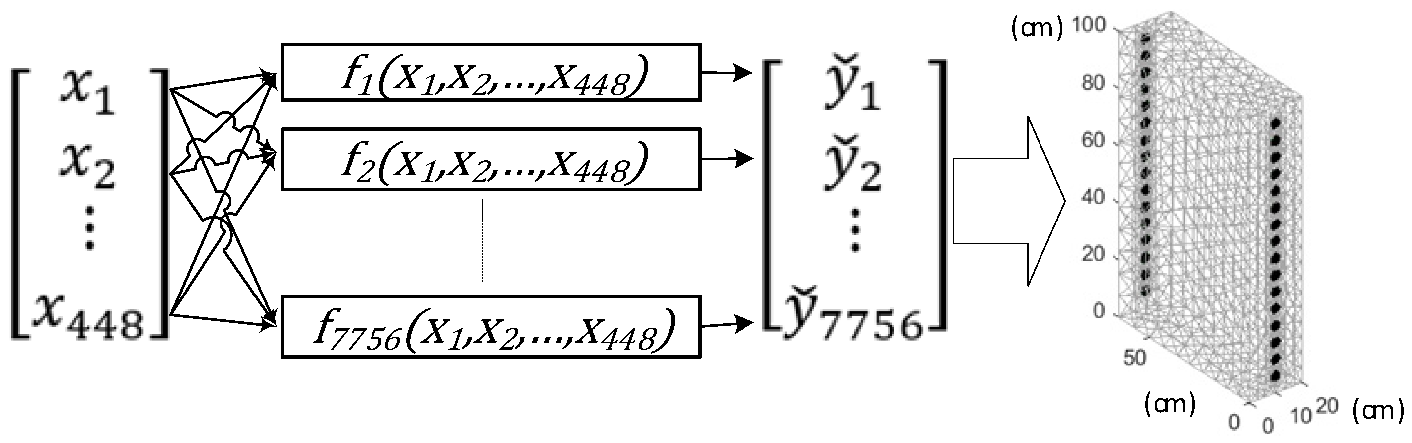
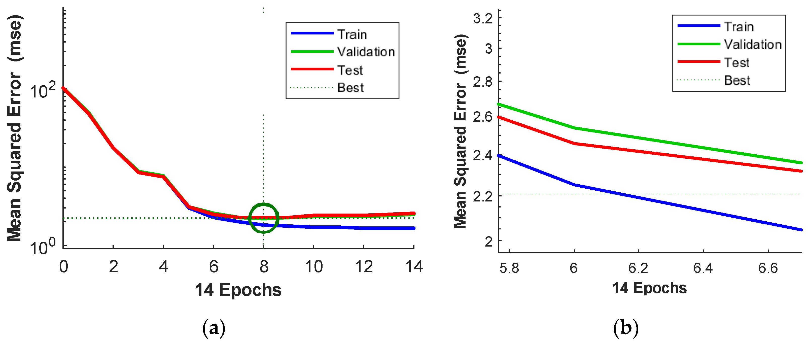
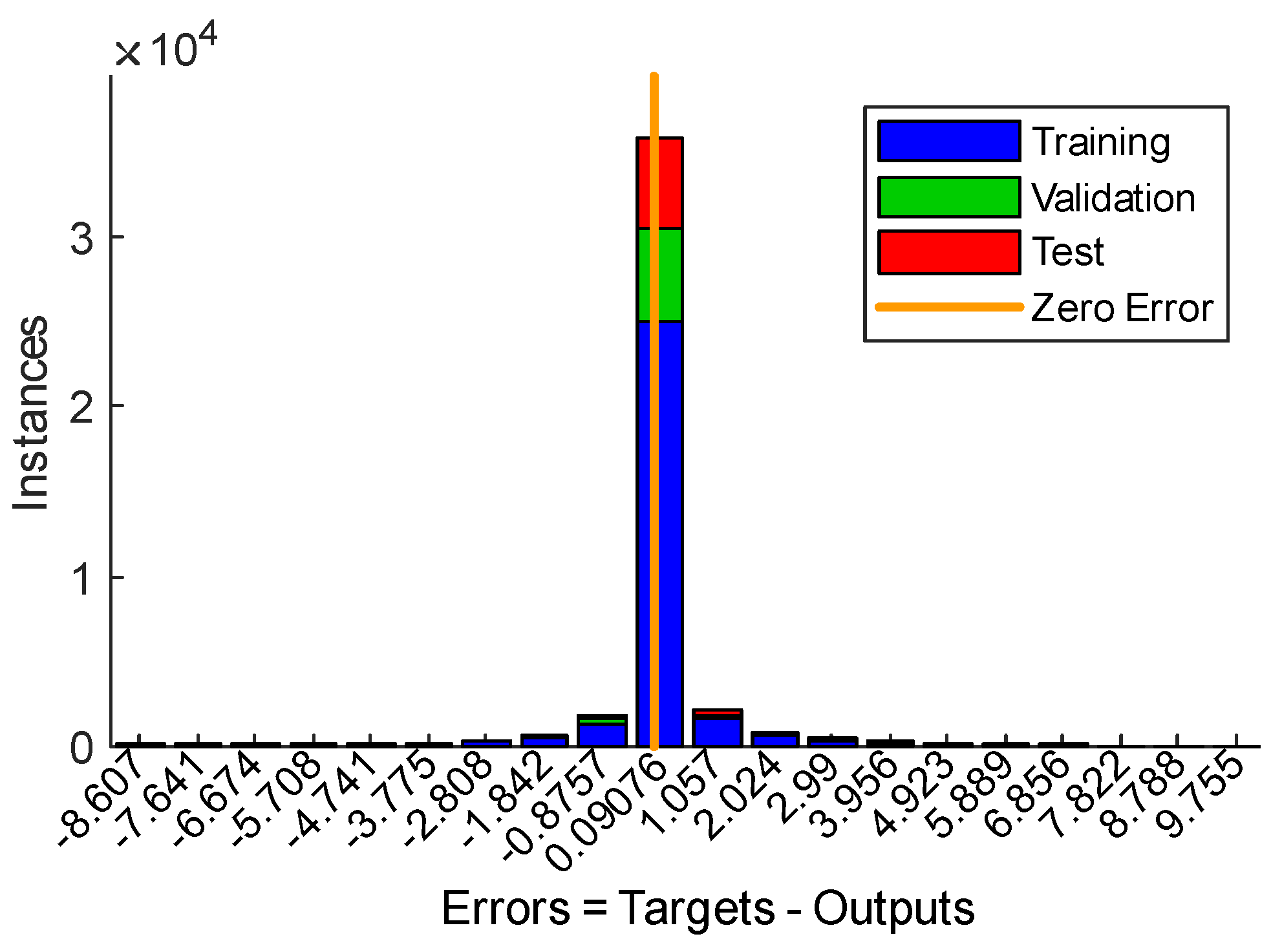
2.3.4. Artificial Neural Network

The research also used artificial neural networks (ANN) in the form of multilayer perceptrons. Since the concept under test involves the use of multiple ANNs, each with a single regression output, there is no reason to overcomplicate the ANNs structure. Each of the applied networks has 448 measurements at the input, 12 neurons in the dictated layer and one neuron in the output layer. Its structure is defined in 448-12-1. In the hidden layer, a hyperbolic tangent $\tanh (x)=\frac{e^{2x}-1}{e^{2x}+1}$ was used as a transfer function, while the output layer uses a linear activation. Neural networks were trained using backward propagation of errors algorithm with conjugate gradients.

The total number of cases used in the network learning process was 44,000. All cases were randomly divided into 3 sets: training (30,800 cases), validation and test (6600 cases each), in the proportions: 70%, 15%, 15%. The training set covers as much as 70% of all cases, because its task is to provide basic information taken into account by transfer functions, on the basis of which the weights and deviation values are determined during the process of learning the artificial neural network (ANN). Cases belonging to the test set and the validation set are not directly involved in the learning process. In the training algorithm used, the task of the validation set was to prevent overfitting, and thus provide the network with the possibility of generalization. Using the early stopping method, the training algorithm computed the MSE error for the validation set. If the validation error increases over the next six epochs, then the network training process is interrupted.

Table 3. The results of the learning process along with the division of data into sets.

Division of Data into Sets	Number of Cases in a Given Set	Mean Square Error (MSE)	Regression (R)
Training set (70%)	30,800	1.80529	0.953182
Validation set (15%)	6600	2.20707	0.942070
Testing set (15%)	6600	2.26530	0.940561

shows the results of the learning process along with the division of data into sets.

Regression R is calculated according to $R\left({\widehat{\delta }}^{\prime }-{\widehat{\delta }}^{\ast }\right)=\frac{cov\left({\widehat{\delta }}^{\prime },{\widehat{\delta }}^{\ast }\right)}{{\widehat{\delta }}_y^{\prime }{\widehat{\delta }}_y^{\ast }}$ where${\widehat{\delta }}_{y^{\prime }}$ is the standard deviation of the reference values and ${\widehat{\delta }}_{y^{\ast }}$ is the standard deviation of the estimated values.

Figure 9a,b show the MSE values calculated for each iteration for the training, validation and test sets. In this case $\mathrm{MSE}=\frac{1}{n}{\displaystyle \sum }_{i=1}^n{\left({\widehat{\delta }}_i^{\prime }-{\widehat{\delta }}_i^{\ast }\right)}^2$ where n is a number of cases in the given set type, ${\widehat{\delta }}_i^{\prime }$ is the reference value of the deviation of the i-th case, and ${\widehat{\delta }}_i^{\ast }$ is the forecast value of the deviation of the i-th case. As can be seen, all three lines are concurrent and have a shape resembling a simple hyperbola, indicating that the ANN is not overfitted. All three lines are very close to each other, which also proves the suitability of network learning. The vertical dashed line indicates the iteration followed by the automatic stop of the learning process. In the analyzed case, learning stops after iteration number 8.

Figure 10 shows a histogram of errors arising in the learning process of the neural network. The shape of the histogram resembles a normal distribution, which is favorable. The greatest number of deviations for all 3 types of sets (training, validation and test) are close to zero. Figure 11 shows the values of the gradient for individual iterations of the validation set in relation to the number of successive increases in MSE for this set. This is important for the overfitting prevention (early stopping method), because after 6 consecutive increases in MSE validation error, the ANN learning process is terminated.

As you can see, iteration 8 is the one after which the MSE has not decreased for 6 consecutive steps. The error gradient decreases for most of the subsequent iterations, and the momentum index has dropped to almost zero after all iterations. The last (lowest) curve of the plot presents 14 epochs, including 6 consecutive epochs that did not improve the validation error. It was assumed that if the validation error does not decrease after the next six epochs, the learning is terminated. Therefore, the learning process ends up in epoch 8. All this confirms the good quality of the network and gives a solid basis for believing that the trained network has achieved a high generalization capacity.

3. Results

This section presents the results of the research on the level of moisture in the internal pillar obtained based on the performed EIT measurements. The first part presents reconstructive images obtained with the use of classical methods and machine learning based on real measurements. The tomographic reconstructions allow a visual comparison of 3D images acquired because of the use of various machine-trained algorithms.

The second part of this chapter presents the ranking of algorithmic methods based on criteria expressed using four objectives, quantitative indicators: root mean square error (RMSE), relative image error (RIE), percentage error (PE), and image correlation coefficient (ICC). For this purpose, simulation measurement data was used. The simulation data allows for assigning the generated reconstruction images to the reference images, which is a necessary condition for supervised training. With reference images and reconstructed images, correlation and deviation ratios can be calculated, which in turn allows the comparison and objective evaluation of algorithmic methods in EIT applications.

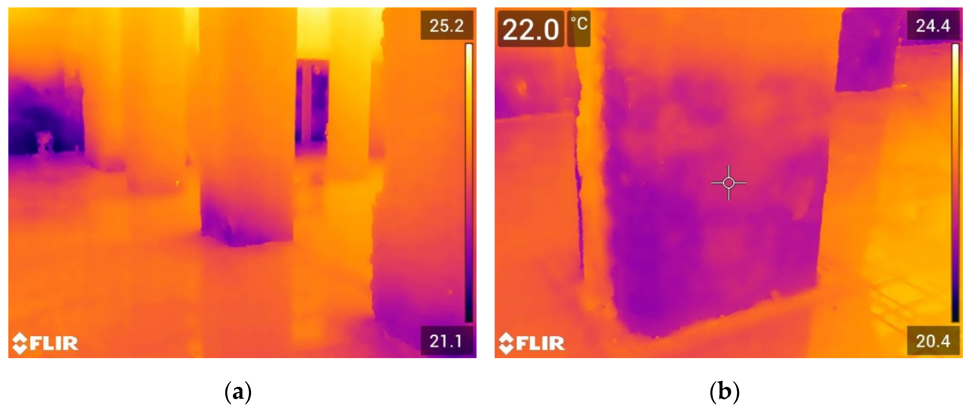
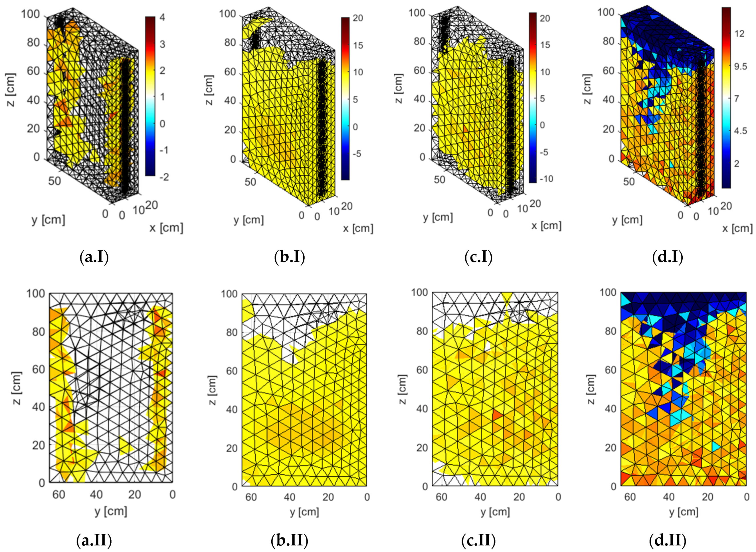
3.1. Visualizations of Real Measurements

Figure 12 shows reconstructive tomographic images of the internal pillar (see Figure 3) obtained by four different methods. All images were created on the basis of the same set of real measurements. Figure 12 consists of 8 individual images. Images (a.I) and (a.II) show the results obtained by using the classical GN algorithm. Images captioned with (*.I) show the 3D views of the tested pillar section, while images captioned with (*.II) show the side views with the electrodes on the right and left. The results obtained with the use of three machine learning methods are presented in a similar way: LR-SVM—images (b.I) and (b.II), LR-LS—images (c.I) and (c.II), ANN—images (d.I) and (d.II).

When comparing the obtained images, it can be seen that the greatest diversity is seen in the reconstructions (d.I) and (d.II) obtained by the ANN method. The highest level of moisture is observed in the lower parts of the pillar, right next to the ground. Moisture remains up to a level of about 80 cm, but only closer to the surface. The inside of the pillar is less damp than its outside, more or less above the level of 40 cm.The reconstructions obtained with the LR-SVM (b.I, b.II) and LR-LS (c.I, c.II) methods look quite similar. They show a large area of moisture from the ground up to the level of about 80 cm. The LR-SVM method is more reliable here because the existence of dry areas close to the ground, as we can see in the images obtained by the LR-LS method, is unlikely.

Reconstruction made with the classical method of GN shows the least amount of damp areas among all tested methods. Moisture areas are located close to the outer surfaces of the pillar (a.I, a.II). The images also show no moisture close to the ground, which seems unlikely.

In the case of tomographic reconstructions obtained based on real measurements [31], there is a problem of the lack of a reference image. Therefore, it is not possible to say with certainty which image is the most reliable. However, in this case, validation studies were performed for the tested pillar section, which is detailed in Section 2.2. Validation studies were carried out using traditional methods, so they were off a point/spot character.

Table 2 shows that the number of measuring points on each side of the pillar was 9 for both the dielectric and microwave methods. In turn, using the gravimetric method, only 2 measurements were made on each side of the pillar. In total, 40-point measurements were made using all 3 methods, of which 36 measurements were made on the surface of the pillar ($U_m^D$ and $U_m^D$) and 4 measurements ($U_m$) a few centimeters below its surface. It is worth noting that the 3D tomographic image consists of 7756 finite elements (pixels) that arise because of the transformation of 448 voltage measurements. It is obvious that 40-point measurements are not enough to get any EIT spatial image. Especially seeing that the measuring points for the dielectric and microwave methods were the same, so the number of measuring points (spots) is limited to 9 ($U_m^D$ and $U_m^D$) + 2 ($U_m$) = 11 on each side of the pillar. On both sides of the pillar (7A and 7B), the total number of measurement points is 22. The classic methods of point measurements make it possible to determine the percentage of masonry moisture at the designated points. However, they do not enable the determination of the spatial distribution of moisture inside the investigated wall section. It should be clarified here that the purpose of the EIT is not to determine the percentage of the water content of the finite elements included in the image mesh. The real objective of the EIT is to visualize the wet areas inside the wall. The reconstruction should primarily indicate zones that are wetter than the background. Background means dry masonry and all values less than or equal to the background (color and value) are also considered dry. Likewise, pixel values higher than the background are considered damp. In EIT, each pixel of the output image is assigned an electrical conductance value, which is reflected by a certain color. With reference measurements that can be easily simulated, there is no problem with determining the background conductance. Most often, colors are calibrated (that is, the conductivity values are assigned to the colors) in such a way that the background moisture is shown in white. The other colors are usually assigned analogously to the colors of the white light spectrum. Yellow, orange and red colors are assigned to higher conductance values. Blue and purple indicate values below the background level.

In the case of images made based on real measurements, the situation is more complicated because we do not have a reference image. Based on 40 validation measurements, it is possible to determine the percentage humidity in 22 points of the tested pillar. By analyzing the information obtained in this way, it is possible to estimate, quite generally, how the humidity of the wall changes depending on the distance from the floor. Due to the lack of reference images and the different purposes of EIT imaging, which is to visualize the spatial distribution of moisture inside the pillar, the use of validation measurements relies on visually comparing the moisture charts (Figure 5) with the EIT images presented in Figure 12. The quantitative assessment of reconstructions, based on quantitative indicators, is presented in Figure 13 and Figure 14, and in

Table 4. Indicators characterizing the quality of reconstruction for individual methods and variants.

Indicator	Methods of Reconstruction
	GN	LR-SVM	LR-LS	ANN
RMSE	4.3799	1.7329	1.8647	0.7428
RIE	0.7944	0.3143	0.3382	0.1347
PE	79%	31%	34%	14%
ICC	0.5542	0.9077	0.8915	0.9836

.

Figure 5 shows that the highest level of humidity was recorded on the ground. Pillar humidity decreases with increasing distance from the floor level. Considering the validation measurements, the reconstructions obtained with the ANN method look the most correct, and the images generated with the GN method the least reliable.

It can be seen that the individual reconstructions have their own colorbars. The lower the numerical value marked on the colorbar, the lower the moisture content. Taking into account the validation measurements, the reconstructions obtained with the ANN method look the most correct, and the images generated with the GN method the least reliable.

The individual reconstructions have their own color scales. This is because each method required individual color calibration for real measurements. Color calibration was performed in order to best visualize wet areas against the background of dry zones. As simulation data were used to train the models that convert the measurements to images, obtaining clear reconstructions based on actual measurements presents a significant challenge. Therefore, individual color calibration turned out to be indispensable.

It is worth noting that the primary purpose of EIT imaging is not to accurately estimate the level of humidity inside the pillar but to identify areas exceeding a certain moisture threshold. To enable the best possible identification of moisture, the color scale was individually selected for each of the four methods.

3.2. Comparison of Methods Based on Simulation Data

Generating simulation data enables the use of machine learning-based methods. In the presented research, three such methods were used: LR-SVM, LR-LS and ANN. Due to a large number of inputs and outputs, successfully training the machine learning models required very large data sets that would be virtually impossible to obtain with manual measurements. In addition, supervised learning requires reference images that are unattainable when performing real measurements. All these arguments prove that in order to train models that work based on machine learning methods, it is necessary to generate a lot of training data first. The method of generating the training data is described in detail in [3].

Generally speaking, a simple problem must first be solved by transforming the conductivity of finite elements distributed over a dense mesh into a voltage measurement vector. Then, the inverse problem should be solved by converting the previously obtained voltages into conductivity values of finite elements distributed on a sparse mesh. As can be seen, two types of finite element mesh need to be developed—dense (for a simple problem) and sparse (for an inverse problem). Both the simple and the inverse problems are solved by the generalized Laplace equation [3].

Figure 13a shows a dense mesh of finite elements with simulated dampness of the pillar from the ground up to 30 cm above floor level.

Figure 13b shows a sparse mesh of finite elements with the same moisture content, while Figure 13c shows a plot of simulated voltages for each of 448 measurements for moisture at a height of 30 cm. Negative measurement voltages result from the different polarity of the electrodes. Figure 14 is analogous to Figure 12. It shows the EIT reconstructions obtained on the basis of simulation measurements for all four tested methods. The pattern image corresponding to the moisture content of the pillar from the floor up to 30 cm are presented in Figure 13a,b. For simulation measurements, all four methods were calibrated in the same color. Therefore, all images refer to a single colorbar. Thanks to this, it is possible to make a fair comparison of methods not only on the basis of quantitative indicators but also taking into account visual, subjective qualitative impressions.

A visual comparative analysis leads to similar conclusions as in the case of reconstructions based on real measurements (see Figure 12). The most similar to the reference image are the reconstructions obtained with the ANN method (d.I, d.II). The image shows a clear border separating the dry zone from the wet zone at a level close to 30 cm on the “z” axis. The reconstructions made with the LR-SVM (c.I, c.II) and LR-LS (c.I, c.II) methods look somewhat decent. The moisture limit here runs over 40 cm. The LR-LS method also generated slight noise, as indicated by artifacts at the level of 100 cm of the “z” axis. The reconstruction made with the classical GN method is definitely the worst. The boundary between the wet and dry zones is jagged, and the wet area is ambiguous.

As mentioned before, the assessment of the quality of the reconstruction based on the images is largely subjective and therefore imprecise. In order to increase the accuracy of the method quality assessment, four popular quantitative indicators were used: root mean square error (RMSE), relative image error (RIE), percentage error (PE), and image correlation coefficient (ICC). The RMSE can be calculated with the use of the Equation (7)

$$\mathrm{RMSE}=\sqrt{\frac{{{\displaystyle \sum }}_{i=1}^N{\left(y_i-{\widehat{y}}_i\right)}^2}{N}}$$

(7)

where: $y_i$—the reference conductivity of i-th pixel, ${\widehat{y}}_i$—the reconstruction conductivity of i-th pixel, N—the number of finite elements in the mesh or resolution of the reference/reconstruction image.

Tomographic images are considered as sets, so their norms can be used to determine the relative error. An example of an indicator that describes a relative error is the RIE. It can be calculated according to Equation (8)

$$\mathrm{RIE}=\frac{\parallel \widehat{g}-g\parallel }{\parallel g\parallel }$$

(8)

where: $g$—the ground-truth (reference) conductivity distribution and $\widehat{g}$—the reconstructed conductivity distribution.

The third indicator used is the relative percentage error that is calculated according to the formula $\mathrm{PE}=\mathrm{RIE}\times 100\%$.

The fourth indicator used to assess the quality of the reconstruction is the ICC. This metric is similar to Pearson’s correlation coefficient. It specifies the similarity between the reference image and the reconstruction and can be calculated according to the Equation (9)

$$\mathrm{ICC}=\frac{{{\displaystyle \sum }}_{i=1}^N\left(y_i-\overline{y}\right)\left({\widehat{y}}_i-\overline{\widehat{y}}\right)}{\sqrt{{{\displaystyle \sum }}_{i=1}^N{\left(y_i-\overline{y}\right)}^2{{\displaystyle \sum }}_{i=1}^N{\left({\widehat{y}}_i-\overline{\widehat{y}}\right)}^2}}$$

(9)

where: $\overline{\widehat{y}}$—the mean conductivity distribution of the reconstructed image, $\overline{y}$—the mean ground-truth conductivity distribution of the reference image.

The smaller the values of the RMSE, RIE, and PE, the better the quality of the tomographic image. ICC = 1 means the perfect correlation of the output image with the reference image, which translates into a more accurate reconstruction. ICC = 0 means no correlation.

Table 4 presents the values of the above indicators calculated for all four algorithmic methods of EIT image reconstruction. It can be noticed that there is a high agreement among all the indicators used, which clearly indicates the highest effectiveness of ANN and the lowest effectiveness of the GN method, which is not included in the group of machine learning methods. An interesting observation is also that all machine learning methods (ANN, LR-SVM and LR-LS) give better results than the classical GN method.

Another observation is the relatively large numerical differences of individual indicators. For example, the RMSE for GN is more than twice as high as for LR-SVM and LR-LS, and almost six times as high as for ANN. The ICC correlation for PE does not exceed 0.6, and for all machine learning methods it is close to 0.9 or in the case of ANN it is close to 1. The conclusions from the analysis of the indicators in Table 4 suggest that machine learning methods have a greater potential for applications in electrical tomography for research humidity of walls than classical mathematical methods, an example of which is the GN method.

4. Conclusions

This article presents research on the effectiveness of the use of machine learning methods to detect the humidity of building walls with the use of EIT electrical tomography. The quality of the four methods was compared. The first of those compared was the Gauss–Newton (GN) method. It represents classical methods that have been known for several dozen years. The next two methods, LR-SVM and LR-LS, are based on linear regression and differed only in the learner used. The last, fourth method, was an artificial neural network (ANN). As you can see, the last three methods are representatives of machine learning.

Thanks to such chosen methods, it was possible to verify the usefulness of machine learning methods in tomographic testing of building humidity, but also to check which of the methods gives the best results, whether models using linear regression are more effective than others, and how machine learning methods fare against the classical GN method. In order to fully answer the above questions, the verification of the methods was carried out on both real measurements and simulation-generated data.

In the presented research, special attention was paid to the verification of the tested methods with the use of real measurements. To make this possible, detailed validation measurements were performed. For this purpose, as many as three conventional methods were used: gravimetric, dielectric and microwave. Thanks to the conducted measurements, line graphs of humidity were developed, which served as a comparison for the reconstruction images obtained on the basis of real measurements. The obtained results indicate that the reconstructions most faithfully reflecting the results obtained thanks to the validation measurements were obtained using the ANN. Linear regression models fare slightly poorer, and the classic GN method the worst.

The same conclusions can be drawn from the analysis of the results of reconstructive experiments based on the simulation data. The use of simulation data made it possible to calculate quantitative indicators, RMSE, RIE and PE errors and ICC regression. All these indicators clearly show that the best simulation reconstructions were also taken with the ANN, and all three tested methods of machine learning are superior to the classical GN method.

It is worth mentioning that in real conditions, an equally important element of an electric tomograph is electronic equipment (tomograph and multiplexer) and properly designed electrodes. Without properly selected current-voltage parameters and the frequency of voltage changes on individual pairs of electrodes, appropriate quality measurements cannot be achieved. All the necessary hardware components that were used in the tests, i.e., the tomograph, multiplexer and electrodes, were designed and made in the Netrix SA laboratory. In this publication, we only deal with algorithmic methods. Hardware issues will be the subject of future publications.

Our future research will concern the verification of models based on various variants of logistic regression. Due to the high non-linearity of transformations accompanying the solution of the inverse problem, we believe that there is a high probability of success in the application of this type of algorithm.

References

1. Rymarczyk, T.; Kłosowski, G.; Kozłowski, E. A Non-Destructive System Based on Electrical Tomography and Machine Learning to Analyze the Moisture of Buildings. Sensors 2018, 18, 2285. [Google Scholar] [CrossRef] [Green Version]
2. Hola, A. Measuring of the moisture content in brick walls of historical buildings-the overview of methods. In IOP Conference Series: Materials Science and Engineering; Institute of Physics Publishing: Bristol, UK, 2017; Volume 251. [Google Scholar]
3. Rymarczyk, T.; Kłosowski, G.; Hoła, A.; Hoła, J.; Sikora, J.; Tchórzewski, P.; Skowron, Ł. Historical Buildings Dampness Analysis Using Electrical Tomography and Machine Learning Algorithms. Energies 2021, 14, 1307. [Google Scholar] [CrossRef]
4. Banasiak, R.; Wajman, R.; Jaworski, T.; Fiderek, P.; Fidos, H.; Nowakowski, J.; Sankowski, D. Study on two-phase flow regime visualization and identification using 3D electrical capacitance tomography and fuzzy-logic classification. Int. J. Multiph. Flow 2014, 58, 1–14. [Google Scholar] [CrossRef]
5. Garbaa, H.; Jackowska-Strumiłło, L.; Grudzień, K.; Romanowski, A. Application of electrical capacitance tomography and artificial neural networks to rapid estimation of cylindrical shape parameters of industrial flow structure. Arch. Electr. Eng. 2016, 65, 657–669. [Google Scholar] [CrossRef]
6. Kryszyn, J.; Smolik, W. Toolbox for 3D modelling and image reconstruction in electrical capacitance tomography. Inform. Control Meas. Econ. Environ. Prot. 2017, 7, 137–145. [Google Scholar] [CrossRef]
7. Kryszyn, J.; Wanta, D.M.; Smolik, W.T. Gain Adjustment for Signal-to-Noise Ratio Improvement in Electrical Capacitance Tomography System EVT4. IEEE Sens. J. 2017, 17, 8107–8116. [Google Scholar] [CrossRef]
8. Majchrowicz, M.; Kapusta, P.; Jackowska-Strumiłło, L.; Sankowski, D. Acceleration of image reconstruction process in the electrical capacitance tomography 3D in heterogeneous, multi-GPU system. Inform. Control Meas. Econ. Environ. Prot. 2017, 7, 37–41. [Google Scholar] [CrossRef]
9. Wajman, R.; Fiderek, P.; Fidos, H.; Jaworski, T.; Nowakowski, J.; Sankowski, D.; Banasiak, R. Metrological evaluation of a 3D electrical capacitance tomography measurement system for two-phase flow fraction determination. Meas. Sci. Technol. 2013, 24, 065302. [Google Scholar] [CrossRef]
10. Duraj, A.; Korzeniewska, E.; Krawczyk, A. Classification algorithms to identify changes in resistance. Przegląd Elektrotechniczny 2015, 1, 82–84. [Google Scholar] [CrossRef]
11. Szczesny, A.; Korzeniewska, E. Selection of the method for the earthing resistance measurement. Przegląd Elektrotechniczny 2018, 94, 178–181. [Google Scholar]
12. Kłosowski, G.; Rymarczyk, T.; Gola, A. Increasing the reliability of flood embankments with neural imaging method. Appl. Sci. 2018, 8, 1457. [Google Scholar] [CrossRef] [Green Version]
13. Yunus, F.R.M.; Azida, N.A.N.; Nor Ayob, N.M.; Pusppanathan, J.; Jumaah, M.F.; Goh, C.L.; Rahim, R.A.; Ahmad, A.; Md Yunus, Y.; Rahim, H.A. Simulation Study of Bubble Detection Using Dual-Mode Electrical Resistance and Ultrasonic Transmission Tomography for Two-Phase Liquid and Gas. Sens. Transducers J. 2013, 150, 97–105. [Google Scholar]
14. Romanowski, A. Contextual Processing of Electrical Capacitance Tomography Measurement Data for Temporal Modeling of Pneumatic Conveying Process. In Proceedings of the 2018 Federated Conference on Computer Science and Information Systems (FedCSIS), Poznan, Poland, 9–12 September 2018; pp. 283–286. [Google Scholar]
15. Soleimani, M.; Mitchell, C.N.; Banasiak, R.; Wajman, R.; Adler, A. Four-dimensional electrical capacitance tomography imaging using experimental data. Prog. Electromagn. Res. 2009, 90, 171–186. [Google Scholar] [CrossRef] [Green Version]
16. Tong, G.; Liu, S.; Liu, S. Computationally efficient image reconstruction algorithm for electrical capacitance tomography. Trans. Inst. Meas. Control 2019, 41, 631–646. [Google Scholar] [CrossRef]
17. Babout, L.; Grudzień, K.; Wiącek, J.; Niedostatkiewicz, M.; Karpiński, B.; Szkodo, M. Selection of material for X-ray tomography analysis and DEM simulations: Comparison between granular materials of biological and non-biological origins. Granul. Matter 2018, 20, 38. [Google Scholar] [CrossRef] [Green Version]
18. Mikulka, J. GPU-Accelerated Reconstruction of T2 Maps in Magnetic Resonance Imaging. Meas. Sci. Rev. 2015, 15, 210–218. [Google Scholar] [CrossRef] [Green Version]
19. Krawczyk, A.; Korzeniewska, E. Magnetophosphenes–history and contemporary implications. Przegląd Elektrotechniczny 2018, 1, 63–66. [Google Scholar] [CrossRef]
20. Soleimani, M.; Adler, A.; Dai, T.; Peyton, A.J. Application of a single step temporal imaging of magnetic induction tomography for metal flow visualisation. Insight Non Destr. Test. Cond. Monit. 2008, 50, 25–29. [Google Scholar] [CrossRef] [Green Version]
21. Kozlowski, E.; Rymarczyk, T.; Klosowski, G. Logistic regression application to image reconstruction in UST. In Proceedings of the 2019 Applications of Electromagnetics in Modern Engineering and Medicine, PTZE, Janow Podlaski, Poland, 9–12 June 2019. [Google Scholar]
22. Rymarczyk, T.; Kozłowski, E.; Kłosowski, G.; Niderla, K. Logistic Regression for Machine Learning in Process Tomography. Sensors 2019, 19, 3400. [Google Scholar] [CrossRef] [PubMed] [Green Version]
23. Kabanikhin, S.I. Definitions and examples of inverse and ill-posed problems. J. Inverse Ill-Posed Probl. 2008, 16, 317–357. [Google Scholar] [CrossRef]
24. Jasiulewicz-Kaczmarek, M.; Antosz, K.; Wyczółkowski, R.; Mazurkiewicz, D.; Sun, B.; Qian, C.; Ren, Y. Application of MICMAC, Fuzzy AHP, and Fuzzy TOPSIS for Evaluation of the Maintenance Factors Affecting Sustainable Manufacturing. Energies 2021, 14, 1436. [Google Scholar] [CrossRef]
25. Kozłowski, E.; Mazurkiewicz, D.; Żabiński, T.; Prucnal, S.; Sęp, J. Assessment model of cutting tool condition for real-time supervision system. Eksploat. I Niezawodn. Reliab. 2019, 21, 679–685. [Google Scholar] [CrossRef]
26. Liu, S.; Jia, J.; Zhang, Y.D.; Yang, Y. Image Reconstruction in Electrical Impedance Tomography Based on Structure-Aware Sparse Bayesian Learning. IEEE Trans. Med Imaging 2018, 37, 2090–2102. [Google Scholar] [CrossRef] [Green Version]
27. Liu, D.; Zhao, Y.; Khambampati, A.K.; Seppänen, A.; Du, J. A Parametric Level set Method for Imaging Multiphase Conductivity Using Electrical Impedance Tomography. IEEE Trans. Comput. Imaging Comput. Imaging 2018, 4, 552. [Google Scholar] [CrossRef]
28. Liu, S.; Wu, H.; Huang, Y.; Yang, Y.; Jia, J. Accelerated Structure-Aware Sparse Bayesian Learning for Three-Dimensional Electrical Impedance Tomography. IEEE Trans. Ind. Inform. 2019, 15, 5033–5041. [Google Scholar] [CrossRef]
29. Liu, S.; Huang, Y.; Wu, H.; Tan, C.; Jia, J. Efficient Multitask Structure-Aware Sparse Bayesian Learning for Frequency-Difference Electrical Impedance Tomography. IEEE Trans. Ind. Inform. 2021, 17, 463–472. [Google Scholar] [CrossRef]
30. Rymarczyk, T.; Kozłowski, E.; Tchórzewski, P.; Kłosowski, G.; Adamkiewicz, P. Applying the logistic regression in electrical impedance tomography to analyze conductivity of the examined objects. Int. J. Appl. Electromagn. Mech. 2020, 64, S235–S252. [Google Scholar] [CrossRef]
31. Rymarczyk, T.; Oleszek, M.; Szumowski, J.; Tchorzewski, P.; Adamkiewicz, P.; Sikora, J. A hybrid tomography system for the analysis of wall dampness. In Proceedings of the 2018 Applications of Electromagnetics in Modern Techniques and Medicine, PTZE, Racławice, Poland, 9–12 September 2018; pp. 220–223. [Google Scholar]
32. Jauhiainen, J.; Kuusela, P.; Seppanen, A.; Valkonen, T. Relaxed gauss-newton methods with applications to electrical impedance tomography. SIAM J. Imaging Sci. 2020, 13, 1415–1445. [Google Scholar] [CrossRef]
33. Jin, B.; Maass, P. An analysis of electrical impedance tomography with applications to Tikhonov regularization. ESAIM Control Optim. Calc. Var. 2012, 18, 1027–1048. [Google Scholar] [CrossRef] [Green Version]
34. Ho, C.H.; Lin, C.J. Large-scale linear support vector regression. J. Mach. Learn. Res. 2012, 13, 3323–3348. [Google Scholar]
35. Hsieh, C.J.; Chang, K.W.; Lin, C.J.; Keerthi, S.S.; Sundararajan, S. A dual coordinate descent method for large-scale linear SVM. In Proceedings of the 25th International Conference on Machine Learning, Helsinki, Finland, 5–9 July 2008; pp. 408–415. [Google Scholar]
36. Xiao, L. Dual averaging methods for regularized stochastic learning and online optimization. J. Mach. Learn. Res. 2010, 11, 2543–2596. [Google Scholar]
Figure 1. Research object—Bastion Sakwowy in Wrocław: (a) lower building (Peristyle Pavilion) where the research was carried out, (b) a research stand with a tomograph in the foreground.
Energies 14 02777 g001
Figure 2. Arrangement of measurement spots on selected elements subjected to humidity tests. The tested pillar is marked in yellow. The arrows and the number-letter symbols indicate the spots and sides of the walls/pillars that were subject to the tests.
Energies 14 02777 g002
Figure 3. The building of the Heimann’s Foundation in Wrocław: internal pillar with EIT electrodes on opposite sides.
Energies 14 02777 g003
Figure 4. Arrangement of measurement points and EIT electrodes for the opposite sides 7A and 7B of the pillar.
Energies 14 02777 g004
Figure 5. Validation of the internal pillar moisture by dielectric, microwave, and mass/invasive methods: (a)—side 7A, (b)—side 7B.
Energies 14 02777 g005
Figure 6. Thermal images of internal pillars: (a)—several pillars, (b)—single pillar.
Energies 14 02777 g006
Figure 7. Model of the multiple EIT system converting electrical signals into 3D image pixel-by-pixel.
Energies 14 02777 g007
Figure 8. Validation of internal pillar moisture content: (a)—objective function model, (b)—Min objective vs. Number of function evaluations.
Energies 14 02777 g008
Figure 9. Validation performance through MSE: (a)—best validation performance MSE = 2.2071 at epoch 8, (b)—close-up of a section of Figure 9a.
Energies 14 02777 g009
Figure 10. Error (MSE) histogram with 20 bins.
Energies 14 02777 g010
Figure 11. Training state through gradient and momentum (mu).
Energies 14 02777 g011
Figure 12. Reconstructions obtained from real measurements: (a.I) and (a.II) refers to GN, (b.I) and (b.II) refers to LR-SVM, (c.I) and (c.II) refers to LR-LS, (d.I) and (d.II) refers to ANN.
Energies 14 02777 g012
Figure 13. Generating simulation data on finite element meshes: (a) dense mesh, (b) sparse mesh, (c) voltage distribution for individual measurements.
Energies 14 02777 g013
Figure 14. Reconstructions obtained from simulation measurements: (a.I) and (a.II) refers to GN, (b.I) and (b.II) refers to LR-SVM, (c.I) and (c.II) refers to LR-LS, (d.I) and (d.II) refers to ANN.
Energies 14 02777 g014