Article

A Wind Energy Supplier Bidding Strategy Using Combined EGA-Inspired HPSOIFA Optimizer and Deep Learning Predictor

1
College of Mechatronics and Control Engineering, Shenzhen University, Shenzhen 518000, China
2
Department of Business Studies, Namal Institute Mianwali, Mianwali 42201, Pakistan
3
School of Engineering, RMIT University, Melbourne 3000, Australia
4
School of Engineering, Macquarie University, Sydney 2019, Australia
5
Department of Electrical and Computer Engineering, COMSATS University Islamabad, Wah Cantonment 47040, Pakistan
6
1 LRIT Laboratory, Faculty of Sciences, Mohammed V University, 10056 Rabat, Morocco
*
Author to whom correspondence should be addressed.
Energies 2021, 14(11), 3059; https://doi.org/10.3390/en14113059
Submission received: 15 April 2021 / Revised: 8 May 2021 / Accepted: 11 May 2021 / Published: 25 May 2021

Abstract

:
As the integration of large-scale wind energy is increasing into the electricity grids, the role of wind energy suppliers should be investigated as a price-maker as their participation would influence the locational marginal price (LMP) of electricity. The existing bidding strategies for a wind energy supplier faces limitations with respect to the potential cooperation, other competitors’ bidding behavior, network loss, and uncertainty of wind production (WP) and balancing market price (BMP). Hence, to solve these problems, a novel bidding strategy (BS) for a wind power supplier as a price-maker has been proposed in this paper. The new algorithm, called the evolutionary game approach (EGA) inspired hybrid particle swarm optimization and improved firefly algorithm (HPSOIFA), has been proposed to handle the bidding issue. The bidding behavior of power suppliers, including conventional power suppliers, has been encoded as one species to obtain the equilibrium where the EGA can explore dynamically reasonable behavior changes of the opponents. Each species of behavior change has been exploited by the HPSOIFA to improve the optimization solutions. Moreover, a deep learning algorithm, namely deep belief network, has been implemented for improving the accuracy of the forecasting results considering the WP and BMP, and the uncertainty revealed in the WP and BMP has been modeled by quantile regression (QR). Finally, the Shapley value (SV) has been calculated to estimate the benefits of cooperative power suppliers. The presented case studies have verified that the proposed algorithm and the established bidding strategy exhibit higher effectiveness.

1. Introduction

With the decline of fossil fuel-generated electricity, people became more and more conscious of the importance of renewable energy. Consequently, welfare policy in recent years that heartens the application of wind energy as a type of renewable resource has been advocated to lessen energy shortage [1,2,3,4]. Under this background, the latest statistics show that the installed capacity of wind energy in certain regions is growing exponentially, and thus it will influence the locational marginal price (LMP) because of the higher percentage and market power of wind suppliers [5]. In response to that, wind power producers’ bidding has been regarded as a price-maker by practical marker operators, such as China’s Gansu province [6], Electric Reliability Council of Texas (ERCOT) [7], Pennsylvania-New Jersey-Maryland Interconnection (PJM) [8], etc.

1.1. Non-Game Approach

To effectively resolve strategic bidding of a price-maker wind power producer, several methods have been researched in recent years. An optimization problem based on a mathematical program with equilibrium constraints has been employed to optimize the BS on the price-maker producer in [9]. The authors in [10], presented a Stackelberg game model, based on a closed-form concept to analyze the bidding behavior of price-maker wind power producers. An optimization model for a wind power producer based on residual demand curves and wind imbalances has been reported in [11] to detect its effect on prices. A robust model based on the uncertainties for wind power and demand response has been reported in [12] to maximize the robust ability while guaranteeing the expected interest. However, most of the past research with BS for wind power producers neglect the adaptive interaction among the power producers [13]. In general, a game-theory-based method is more suitable for using the BS of market participants as price-maker because it concerns the strategic interactions among power suppliers [14].

1.2. Traditional Game Approach

A game-theory-based method could be based on the traditional game approach or evolutionary game approach (EGA) [15]. The traditional game approach aims to find the Nash equilibrium that can be the best strategy between the power suppliers. The authors in [16], the presented technique used a supply function equilibrium for modeling the impacts of bidding behavior of wind power suppliers. The authors in [17], the models assuming conventional suppliers’ bids as a constant was developed to enhance the interests for a wind supplier, and wind production (WP) and BM price (BMP) were predicted by time series methods to reduce the uncertainty risk in the balancing power market. However, conventional power suppliers’ bids are considered a constant that can be completely unrealistic, because other people’s strategies may change. Moreover, the uncertainty exhibited in the WP and the BMP is usually unacceptably enormous, thus it is difficult to extract the inner features and describe the uncertainty for the WP and the BMP based on traditional predict models. Finally, the conventional game methodology neglects to consequently gain the dynamic offering data of various competitors. This suggests that their offering conduct cannot change an exact reflection that they have learned [18]. Therefore, numerous optimization algorithms dependent on EGA were developed innovatively in different domains [19,20].

1.3. Evolutionary Game Approach (EGA)

The evolutionary game approach (EGA) is a combination of interconnection between the traditional game approach and dynamical arguments such as bat algorithm (BA) [21] and genetic algorithm (GA) [15], which will be able to optimize the profits for conventional power suppliers. So far, a number of research works have been published on EGA-based wind energy bidding. The authors in [21], a meta-heuristic bat-inspired optimal algorithm was proposed to maximize the double-layer model. Here, the higher-layer and the lower-layer models are used to maximize conventional power profits and to solve the market-clearing problems of independent system operators, respectively. An evolutionary imperfect information game approach based on a refined genetic algorithm with price-elastic demand bidding strategies was applied in [15]. However, BA and GA can undoubtedly generate immature convergence through equilibrium solutions. Furthermore, as previously mentioned, the literature fails to account for the cooperative presence and network loss.

1.4. Purposes and Contributions of the Paper

It can be seen from the above discussion that there are some limitations to overcome, although several studies have reported wind energy bidding as a price-maker. In the proposed framework, wind power producers cannot only understand and learn the information of other competitors but also automatically cooperate with rivals to enhance their interests. It has been presented in [22] that cooperative behavior in certain domains can improve the interests of all parties. Hence, the cooperative relationship among the wind power producer should be considered, and the benefit allocation is also analyzed for verifying the existence of the collations. Afterward, the bidding models in previous studies neglect the impact of network loss, whereas network losses (NL) for power systems account for 3–5% of the total power consumption [23]. Most of the well-known electricity markets such as PJM, NYISO (New York Independent System Operator), and MISO (Midwest Independent System Operator) have considered the network loss to better represent power flow characteristics. Therefore, to model the practical operation in the well-known power markets, network loss should be considered for wind energy BS. Moreover, current strategies in the dynamic power market have failed to produce equilibrium solutions, which can oscillate in the solution space and fail to converge [24]. Therefore, an advanced evolutionary approach that can produce a reliable equilibrium solution is highly required. Finally, the traditional algorithms cannot extract the nonlinear features and describe the uncertainty for the WP and the BMP. Hence, the identification of a forecasting framework is critical that will improve the forecasting accuracy and reflect the uncertainty for the WP and the BMP [1].
In summary, to address the above-mentioned challenges, a novel BS for the wind power producers with the uncertainty of WP and BMP is proposed in this paper. This paper contributes in the following aspects:
  • Another bi-layer enhancement model for the wind power makers is proposed here. The top layer depicts the helpful connection between customary power providers and a wind provider with the vulnerability of WP and BMP, and the lower-layer model is the independent system operator’s (ISO) improvement considering losses in the network. The model is targeted for enhancing the profits of the wind power producers;
  • An evolutionary game approach based on a hybrid particle swarm optimization and improved firefly algorithm (HPSOIFA) is newly proposed to tackle the bi-layer bidding model. The methodology can produce a more solid balance arrangement contrasted with conventional techniques;
  • A deep belief network (DBN) is introduced and adjusted to comprehensively extract nonlinear features for the WP and BMP. And the uncertainty in the WP and BMP is probabilistically formulated based on the quantile regression (QR).

1.5. Structure of the Paper

The remainder of this paper is organized as follows. The bi-layer model with the network loss and coalition for wind energy bidding is presented in Section 2. The new solving methodology of EGA-inspired HPSOIFA, DBN, and QR-based probabilistic forecasting, and profit distribution by Shapley value (SV) are represented in Section 3. Case studies are reported in detail in Section 4. Finally, conclusions are drawn in Section 5.

2. Wind Energy Suppliers’ Coalition Model

In this section, a bidding problem for the wind energy suppliers will be discussed. Then, a novel bidding model incorporating network loss and coalitions based on the WP and BMP uncertainty will be proposed.

2.1. Problem Description

The wind energy suppliers in the power market have been changed to the price-maker from the price-taker, which shows that wind energy suppliers in the BS seem to be similar to conventional large power suppliers. However, since wind energy has inherent intermittency and fluctuation, the bidding behavior (BB) for wind energy suppliers will become uncertain. To reduce the uncertainty risk in balancing the power market, knowing the information in advance for wind energy suppliers is crucial in day-ahead market bidding, where wind energy suppliers are permitted to submit energy offer curves at each hour. Therefore, this uncertain information, including the WP and BMP, is considered in this paper and integrated into the wind energy suppliers’ profits. Furthermore, the wind supplier, to some extent, can adopt the BB cooperatively alone or with other market participants to improve their bidding performance. Eventually, network loss (NL) should be considered for wind energy suppliers to satisfy the operational requirements of the electricity market.
Hence, this paper proposes a hierarchical model for the wind power suppliers in the day-ahead market. The top-layer model is to boost the power suppliers’ benefits constituted by co-distributor and non-co-distributor with the uncertainty of the WP and BMP and hence obtaining the value of the BS. Although the lower-layer model focuses on minimizing the overall cost for power suppliers considering network loss, that will determine the LMP for each power supplier.

2.2. The Top-Layer Model

The top-layer model is presented as power suppliers’ profits with cooperative existences in a non-cooperative environment. The BS of the electricity power pool consists of conventional power suppliers I and a wind energy supplier w-who submitted to the ISO. If the conventional power suppliers I 2 and a wind energy supplier w decide not to cooperate with conventional power suppliers I 1 ( I 1 = I I 2 ) , the model top-layer model is described as follows,
l F = max { g i n n , [ o O π w , o f w , o + i c I 1 g i c n ] } f w , o = t = 1 T ( ρ w , t q w , t C w , t ρ w , t b , o q w , t b , o ) g i = t = 1 T ( ρ i , t q i , t C i , t ) C i , t = α i q i , t 2 + β i q i , t + γ i C w , t = c w q w , t o O w π w , o = 1 I = I 1 + I 2 i = i n o r i c g i = g i n n o r g i c n i n = 1 , 2 , , I 2 t = 1 , 2 , T ; o = 1 , 2 , , O
where i and ω denote a conventional power supplier and a wind energy supplier, respectively; the superscript/subscript n and c are the non-cooperative behavior and cooperative behavior, respectively; t is the time index; and π ω , o represent a scenario and its probability; g i represents the profits for conventional power supplier i; f w , o represents the profits for wind energy supplier w in scenario o; ρ i , t ( ρ ω , t ) and q i , t ( q ω , t ) are the LMP and the quantity of awarded generation for supplier i ( ω ) at hour t in the upcoming day market.
In Equation (1) ρ w , t b , o and q w , t b , o are the pricing for the market, and the sale/purchase power to/from the BM for supplier w at hour t in scenario o, respectively. C i , t ( C ω , t ) denotes the cost function for power supplier i ( ω ) at hour t. C ω is the cost coefficient for wind energy supplier ω . α i , β i , and γ i are coefficients of cost for conventional power supplier i. In Equation (1), the first and second equality constraints are the total profits for conventional power supplier i and wind energy supplier ω , respectively. The third and fourth equality constraints denote the operating cost for conventional ith power supplier and wind energy supplier ω at hour t, respectively. The sum of all scenarios’ occurrence rate is shown as the fifth equality constraints, is Equation (1).
Hence, the bidding price [22] for power supplier i ( ω ) at the tth hour can be described in Equation (2).
λ z , s , t = k i , t ( 2 α i ω i , s , t + β i ) z = i k w , t c w ω w , s , t z = w
where ω i , s , t and ω w , s , t are the offer amount of sth segment for energy provider i ( ω ) at hour t. k i , t ( k w , t ) , is the BS for the i ( ω ) power supplier at hour t. Overall, the range of the k i , t , and  k w , t is represented by
k z min k i , t , k w , t k z max
where k z m i n and k z m a x in Equation (3) are boundaries of the BS for energy provider z.

2.3. The Lower-Layer Model

The lower-layer model works in according to the NL and the economic dispatch security-constraint, the ISO has been cleared, if the BS from the top-layer model is submitted to the ISO, which is presented as follows:
min t = 1 T i = 1 I s = 1 S i , t λ i , s , t q i , s , t + s = 1 S w t λ w , s , t o q w , s , t o s . t . s = 1 S i , t q i , s , t = q i , t s = 1 S w , t q w , s , t o = q w , t o i = 1 I q i , t + q w , t o b = 1 B q b , t P l o s s , t = 0 q w , t o = q w , t r , o + q w , t b , o P l o s s , t = ( H t ) T ( i = 1 I q i , t + q w , t o b = 1 B q b , t ) + ψ l , t S F l , t ( q i , t + q w , t o q b , t ) = F l , t p i , t p i , t r i max p i , t p i , t r i min q i min q i , t q i max q w min q w , t r , o q w max F l min F l , t F l max ( t = 1 , 2 , . . . T ; o = 1 , 2 , . . . O )
where the system buses and lines number is represented by L and B in Equation (4) respectively; T and O are the aggregations of time and scenarios; S i , t represents the segments for the ith supplier at the tth hour. λ i , s and q i , s , t in the objective function in Equation (4) are the cost and amount for s segment of conventional ith provider at tth hour; λ w , s , t o and q w , s , t o are the price and the awarded amount for segments s of ω wind supplier at the tth hour in the oth scenario; q b , t represents the node voltage at the b bus at the tth hour; q w , t r , o represent the wind power produced by wind supplier ω at hour t in scenario o; q w t b , o is the power purchased from/sold to the market for w wind supplier at the tth hour in the oth scenario; P l o s s , t denotes the system loss at hour t; H t and ψ l , t representing the sensitivity and linearization offset in system loss at tth hour; S F indicate the shifting factor; F l t is line flow through the lth line at the tth hour; q i m i n and q i m a x are the representing the ith supplier minimum and maximum out. r i m i n and r i m a x are the ith supplier minimum and maximum ramp. F l m i n and F l m a x are the real power flow boundary limit for the lth line; The total awarded generation in the tth hour for supplier is shown in the first and second equality constraints in Equation (4). The power balance constraint is shown in the third equality constraint in Equation (4). The fourth equality constraint representing the total generated power through wind plus the power sale/purchase to the balancing market. More details about the mentioned constraints for CNL could be found and explained in [25].
After clearing the network loss with the SCED model, the Kuhn–Tucker Condition is used to mathematically model the LMP for each supplier which is shown as [25],
ρ t = η t e η t P l o s s , t / q i , t + T l , t T ( γ t + γ t )
In Equation (5) η t is addressing the Lagrangian multiplier for the power boundaries at the tth hour; while forward and in reverse Lagrangian multipliers for the line flow constraint at the tth hour is addressed by γ t + and γ t . From Equation (5), it is also obvious that the LMP is consisting of marginal energy costs, marginal loss, and congestion.

3. Solution Method–Novel Hybrid Optimization Model

In this subsection, the novel hybrid optimization algorithm based on the EGA-inspired HPSOIFA is presented to solve the bidding model for a wind energy supplier. Furthermore, for the first time, a forecasting framework comprising a DBN and a QR is introduced in wind energy bidding. At last, a profit model for cooperative power suppliers is employed by SV (Shapley value) [26].

3.1. Evolutionary Game Approach (EGA)

The evolutionary game approach (EGA), as proposed is the combination of the classical approach and the dynamical arguments with objective as a group of a few rational participants. Compared with the conventional game approach, EGA focuses on the behavior of strategic change instead of the idea of strategic balance. Subsequently, the individual information, conviction, and danger inclination of the members are viewed. The EGA has been used in an assortment of various practical applications [27].
This article uses the EGA as the speculative justification for the market balance, and the HPSOIFA is used to dynamically change their contribution behavior. During the time spent information affiliation, each provider is exhibited as is encoded as one flexible individual, and next smooth out their contribution behavior from learning adversaries’ contribution information by the HPSOIFA.

3.2. Hybrid Particle Swarm Optimization and Improved Firefly Algorithm (HPSOIFA)

The given PSO is a kind of mathematical computational calculation with restricted capacity assessments. It was initially inspired by the regularity of birds’ swarm activity that established a simplified optimization model. In PSO, each individual called particle can learn itself by two tracking extremes, where one is called its personal best position (Pbest) found by its particle, and the other is called the global best solution (Gbest) found by the whole particles. Hence, PSO can have advantages of high speed and global exploration to approach complex optimization problems, because each individual tends to make full use of their own experience and group experience [28,29].
However, the fundamental limitation of PSO, particularly in managing the complex multi-modular capacities, is responsible to deliver untimely convergence, which could be essentially credited to the deficiency of variety in the inquiry space [28]. To tackle these issues, various PSO algorithms have been developed to apply in different areas so far and could generally be divided into two categories, which are: (a) the PSO variant based on the mutation operation and (b) the hybrid PSO with other algorithms. The first method is based on study strategies or neighborhood topologies consisting of teaching and peer learning. However, as analyzed in [30,31], if the mutation operation is only added to PSO to improve the local exploitation, however, its global exploration or convergence rate may be damaged.
Consequently, the second strategy in this paper is used to adjust the trade-off between nearby misuse and worldwide investigation. It tends to be observed from the above examination that PSO might be exposed to untimely intermingling when particles are caught in nearby minima. Despite what is generally expected, the firefly calculation (FA), which was proposed in [32,33] is another computational calculation, which can be designed to conquer this disadvantage, then again, it additionally has a few shortcomings, for example, slow convergence because of the absence of information about the individual optimum [34,35]. Accordingly, a novel cross breed calculation consolidating PSO and improved FA (HPSOIFA) is proposed to use the qualities of every one of them. It ought to be noticed that the searching through the behavior of the FA, known as the full fascination model, is controlled by the attractions among fireflies and every firefly that can be pulled in by any remaining more brilliant fireflies. The existence of excessive attractions in the full attraction model may not be able to perform local search completely and might be caught into a local optimum [36]. Under the circumstances, a chaotic-sequence-based theory is introduced to FA, termed as improved firefly algorithm (IFA), which may enhance local search to escape from local minima, because it has the characteristics of periodicity, randomness, and regularity.

3.2.1. Halton Initialization

A reliably scattered introduction more often than not is sensible for restricted sub-streamlining issues while handling collusion balance for the provider in the market since it could not be unconcerned to the ideal area. Nonetheless, a couple of examinations have found that the Halton point set [37] can convey a more uniform scattering to the entire space populace and present a genuine degree of consistency. Additionally, mathematical estimation for the Halton point set showed the possibility of performance improvement of the algorithm [37]. Accordingly, for the initialization process, Halton point set is introduced which is shown as,
k i , j 0 = k i , d m i n + H a l t o n i i , d × k i , d m a x k i , d m i n i = 1 , 2 , , N P ; d = 1 , 2 , , N d
In Equation (6), k i , d 0 , k i , d m i n and k i , d m a x indicate the starting value, the boundaries of BS for ith supplier. Population size and decision variables dimension is represented by N p , pseudo-random worth gained from the Halton code [37] is N d . H a l t o n i ( i , d ) .

3.2.2. Selected Operator

It can be learned, according to the above analysis, that in standard PSO, there are a few benefits for the global investigation and fast convergence, but from the local search perspective, this hindrance can be completely solved by FA because of its adjusting controls in local exploitation. In this way, particles refreshing in nearby exploitation will execute a FA, if the nearby particles position are better than global one, in any case, then it must be refreshed by the PSO. Mathematically, the determination administrator is represented as
θ i i t e r = 0 p i i t e r > g i t e r 1 1 p i i t e r g i t e r 1
In Equation (7), θ i i t e r represents updated choice pattern for particle i in the iteration i t e r , p i i t e r means the current finding for ith particle in the i t e r cycle. The global solution in the ( i t e r 1 ) t h iteration is represented by g i t e r 1 .

3.2.3. PSO Updation

In each cycle, the particle invigorates itself by following two extrema [28]. The first is basically the ideal arrangement obtained by the real particle, which is known as the individual extreme value, and another limit esteem is the ideal arrangement found by the whole populace, which is the worldwide limit esteem. Consequently, populace invigorates with PSO according to the above suspected can be portrayed as follows,
v i i t e r + 1 = w i t e r v i i t e r + c 1 r 1 ( p i i t e r k i i t e r ) + c 2 r 2 ( g i t e r k i i t e r )
k i i t e r + 1 = k i i t e r + v i i t e r + 1
A random number between 0 and 1 is represented by r 1 and r 2 ; c 1 and c 2 in Equations (8) and (9) denote learning factors; the ith particle velocity vector in the i t e r iteration is represented by v i i t e r ; w i t e r is inertia weight which may be used for the enhancement of convergence rate, given by
w i t e r = ( w 1 w 2 ) ( i t e r max i t e r ) / i t e r max + w 2
In Equation (10), initial weight value is indicated by w 1 and w 2 , while the maximum iteration is represented by i t e r m a x .

3.2.4. IFA Updation

At each cycle, the fireflies can use their attractions to invigorate populace areas. Regardless, the pointless existing attractions between fireflies will convey an influencing that separates the close by availability. As shown by [36], a tumultuous grouping-based theory can assist FA with avoiding some close by neighborhood minima and increase the calculation execution. Properly, the update rule of fireflies is numerically addressed as demonstrated in Equation (11).
k i i t e r + 1 = k i i t e r + r 0 e γ r i j 2 ϑ i t ( k j i t e r k i i t e r ) + a i t e r ξ i t e r
where ϑ i t is the chaotic number and a variable which is calculated according to Equations (12) and (13); ζ t is a random value; r 0 represents the starting attractiveness; k j t denote the brighter firefly from any other firefly; absorption coefficient is represented by γ ; distance between any two firefly is given by r i , j which is calculated from Equation (14). From Equation (15), the changed velocity is calculated on the bases previous.
ϑ i i t e r + 1 = μ ( ϑ i i t e r ) 2 sin ( π ϑ i i t e r )
a i t e r = 1 r a n d ( 1 i t e r / t max ) d r
r i j = k i k j = ( x i x j ) 2 + ( y i y j ) 2
v i i t e r + 1 = k i i t e r + 1 k i i t e r
where the chaos behavior can be control through μ ; in Equation (13) d r represent the decay rate.

3.3. DBN-Based Deterministic and Probabilistic Forecasting of WP and BMP

Traditionally, machine learning methods, such as support vector machine [38], boosting method, and shallow back-propagation neural network, are applied to forecast the WP and BMP. But research findings suggest that high variability and nonlinear characteristic of WP and BMP may not be entirely extracted by conventional methods and may reduce the forecasting accuracy [1]. Consequently, a deep learning method, also known as deep belief network, is adopted and adjusted in this paper for improving the forecasting accuracy of the WP and the BMP. The deep belief network is consisted of several layers of stacked restricted Boltzmann machines (RBM) as its generated module and a layer of logistic regression for forecasting output [39], as shown in Figure 1. Furthermore, the uncertainties exhibited in the WP and BMP are probabilistically evaluated using the quantile regression (QR) [40].

3.3.1. DBN-Based Deterministic Forecasting of WP and BMP

(1) Restricted Boltzmann machines
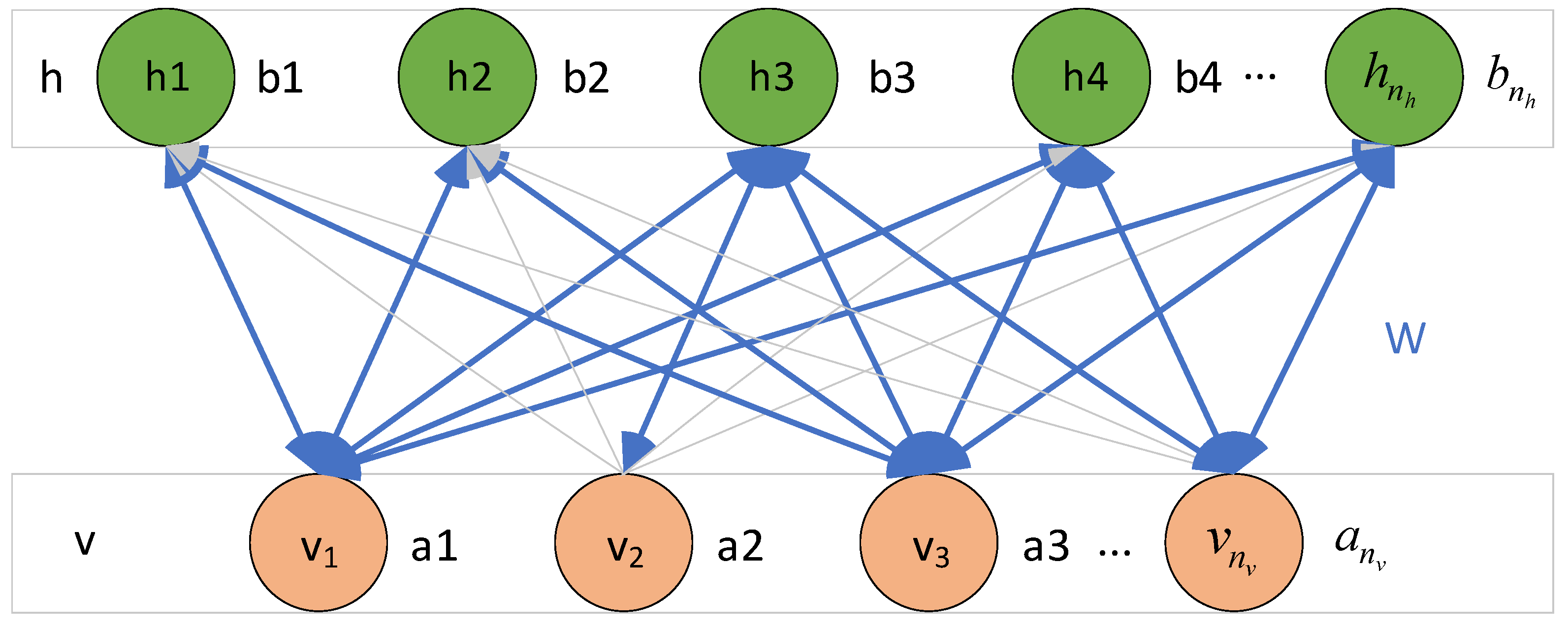
The RBM, as part of the binary DBN network model which includes two layers that are visible layer using accepted inputs and the hidden layer using extracted features. Due to the absence of interconnection among neurons in the hidden layer, while symmetrical connections exist between the neurons in the inter-layer. The advantages are that the values at each hidden unit are uncorrelated if given the visible units, as shown in Figure 2. Hence, the values at each unit are computed simultaneously and in parallel instead of calculated separately. The probability distribution trained by RBM based on an energy function, in this case, would be more effective when compared to the normal Boltzmann machines [41]. The energy function can be mathematically modeled as follows,
E ( v , h ) = a T v b T v h T W
In Equation (16), a and b are the offsets; W is the connection weight. V and h are the states of the visible and hidden layers.
(2) RBM pre-training process
The probability distribution which can be used to produce the samples with the highest probability is the pre-training of RBM. Therefore, the model parameters, including the offsets, a and b, and weights W, should be trained by giving a certain amount of training data to achieve the optimal states, the objective function can be defined as follows,
L θ , S = v S N log ( h E ( v , h ) Z )
where in Equation (17) the partition function is represented by Z. Based on the Bayesian statistics theory [42], the performance metric is maximized by the stochastic gradient method to obtain an RBM with favorable parameters. Therefore, by the derivative of the train function L θ , s , the model parameters a and b, and weights W are updated as follows,
L θ , S L θ , S W W = E P [ h v ] E P * [ h v ]
L θ , S L θ , S a a = v E P * [ v ]
L θ , S L θ , S b b = E P [ h ] E P * [ h ]
where E p [ h v ] and E P * [ h v ] in Equations (18)–(20) are the expected operation for probabilities of the original-data-driving and the reconstructed-data-driving over visible layer v. Nevertheless, the expectation calculations for reconstructed-data-driving probabilities would be difficult to handle because of its expectation distribution learned by the RBM. Recent research finds that an alternative faster method, named contrastive divergence algorithm, is developed to evaluate reconstructed-data-driving probabilities. This algorithm can obtain the expectations of the prediction model with Gibbs sampled process with multiple iterations using each iteration of trained data [42], and the model usually can be fulfilled within an iteration. Therefore, the updated rule for model parameters a , b , and W can be deduced from Equations (21)–(23), as follows,
W t s + 1 = W t s + η P ( h | v ) v T P ( h * | v * ) ( v * ) T
a t s + 1 = a t s + η ( v v * )
b t s + 1 = b + η { p ( h | v ) P ( h * | v * ) }
where the time step and the learning rate are represented by the superscript t s , and  η . The activation probabilities for v given h is P ( h | v ) and h given v is P ( v | h ) .
(3) DBN-based deterministic forecasting framework
The training and learning process of DBN usually divided into two stages: a pre-training process with unsupervised learning using a greedy layer-by-layer form and fine-tuning process with supervised learning using back-propagation (BP). The former means that the output of the hidden layer found on the RBM above is taken as the input of the RBM below, once the states of the above RBM are learned by the pre-training process. The latter is to adjust and optimize parameters of the overall DBN, because each RBM after the pre-training process of DBN cannot be satisfied with the global optimum for the whole RBM, only to the local optimum at its own RBM. More detailed information concerning the BP in DBN can be found and expressed in [43]. Once the model parameters for DBN will be terminally optimized after a certain cycle, the DBN model will be used in the forecasting for WP and BMP.

3.3.2. DBN-Based Probabilistic Forecasting of WP and BMP

Deterministic forecasts will be incapable of evaluating the uncertainties relative to given forecasting of WP and BMP, though a DBN is introduced to improve the forecasting accuracy. However, this uncertainty that can be depicted by probabilistic forecasting plays a very important role in reducing the bidding risk of wind energy suppliers [44]. Generally, traditional solutions for modeling probabilistic WP and BMP from a set of deterministic forecasting may be improper based on an artificial hypothesis in which the acquired errors obey a certain distribution, i.e., Gaussian distribution. Hence, in this paper, quantile regression ( Q R ) [45] without any hypothesis is introduced and estimated via a minimization function, as follows,
min β τ R j ρ τ ( y j x j β τ r )
In Equation (24), y j and x j denote the forecasting and real value for sample j, respectively. β τ is an optimal vector according to τ (quantile value); ρ τ is a piecewise linear loss function, which is defined in Equation (25).
ρ τ = τ r i f r > 0 ( 1 τ ) r o t h e r w i s e
Thereupon, the uncertainty for W P and BMP can be evaluated through Equation (26), once β τ is obtained, as follows,
y τ = β 0 , τ + β 1 , τ

3.4. Shapley Value

The profit distribution of cooperative power suppliers is a crucial problem, which directly affects the stability of long-term cooperative suppliers. The authors in [26], used SV S v z to distribute power suppliers’ profits which is summarized in Equation (27).
S v z = S S c ! ( Z 1 1 S c ) ! Z 1 ! m z ( v )
where S c , in Equation (27) denote a sub-coalition consisting of cooperative power suppliers. m z ( v ) denotes the marginal contribution for power supplier z, defined as follows,
m z ( v ) = v ( S c { z } ) v ( S c )
In Equation (28), v ( S c ) represents the profits for sub-coalition S c . SV S v z can be applied to the profit distribution of cooperative power suppliers with the next two requirements,
z Z 1 S v z = v ( P )
S v z f z n
In Equation (29), the sum of the Shapley values S v z is equal to distributing total profits for cooperative suppliers. It means that cooperative suppliers need to meet the demand of Pareto distribution. In Equation (30), the cooperative profits S v z for power supplier should be greater than non-cooperative profit f z n .

3.5. Proposed Solution Model

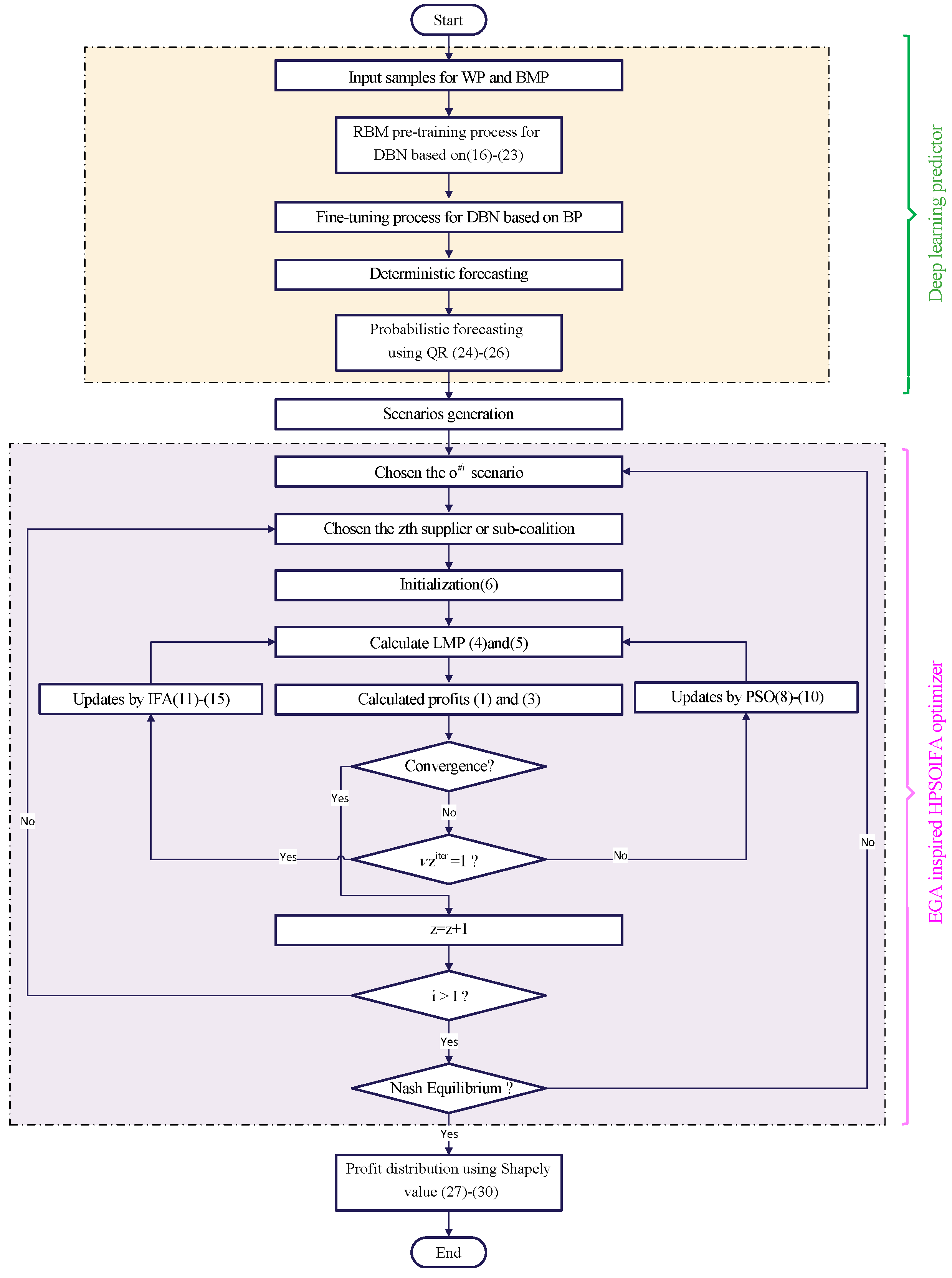
In this article, a bi-layer framework for a power supplier as a price-maker is proposed and the supplier-based BS is modeled as one species. Then, HPSOFAEGA is consists of the EGA, and HPSOIFA is used for the solution of given bidding model. Additionally, a forecasting framework comprising the DBN and QR is introduced to reduce the uncertainty. At last, the benefits of the agreeable suppliers are appropriated by Shapley value. Taking everything into account, the stream diagram for addressing the offering model appears in Figure 3. The Pseudocode the given framework is shown in Algorithm 1.

4. Empirical Results and Discussion

4.1. Experimental Settings

The modified version of the standard IEEE 30 bus system serving as a system model is made up of, 41 transmission lines, 24 load buses, and 6 generators (a wind power supplier and 5 conventional power suppliers), and the grid topology is shown in [46]. Furthermore, a wind power supplier with 45 MW (G1) rated capacity is fixed at bus 1. The remaining conventional power suppliers (G2, G3, G4, G5, and G6) are connected at bus 2, bus 5, bus 8, bus 11, and bus 13, respectively, their corresponding capacity is set to 58 MW, 65 MW, 60 MW, 62 MW, and 60 MW. The wind energy penetration is approximately 14.8% of the installed capacity throughout in the system. This penetration of wind energy is a perfect reflection in the real grid, such as most state systems in the USA. The second-order cost coefficients for conventional power suppliers, which assume that the constant terms are set as 0, are individually set to 0.18, 0.5, 0.067, 0.2, and 0.2, and their corresponding first-order cost coefficients are 14, 9, 26, 24, and 20, respectively. Additionally, the cost coefficient for wind suppliers is set to 8.15. This is obviously below other conventional suppliers with exorbitant marginal costs.
From reference [31], we can obtain the PSO parameters for the HPSOIFA. The underlying weight value of w 1 and w 2 are fixed at 2 and the learning factors c 1 and c 2 is assigned as 3.1 and 2.1 Local searching ability mainly depends upon the parameters of the IFA, i.e., r 0 , γ , μ , and  d r . From [47], the initial attraction distance, i.e.,  r 0 , is assigned a value of 1. The retention coefficient, γ , decides the difference in allure over the long haul. A bigger estimation of γ would slant the unsteadiness of the algorithm and a more modest estimation of γ would slow down the convergence rate. Our investigations show that γ = 1 is more appropriate for the cases introduced in this paper. The chaos behavior is controlled by setting the value of μ as 2.1. The decay rate is decided by the value of d r , i.e., 0.95. The value of N p and i t e r m a x would be ranges from 30 to 60 and 20 to 60, respectively. These values depend on the problem complication, and its value affects the convergence rate.
Algorithm 1 Pseudocode of the wind power producers’ market bidding algorithm
DBN
  • Input:RBM(V, W, H), training and testing set (X, y), the learning rate η , quantile value τ
  • Output:Output: the connection weight, and the uncertainty of WP and BMP Initialize V, W, H=0
1:
for V=1:S do
2:
    V(0)=V
3:
    for ts=0:T do
4:
       Update the connection weights, and the states of the visible and hidden layers using Equations (16)–(23)
5:
    end for
6:
end for
7:
Save the connection weights
8:
Initialize the biases
9:
for V=1:S do
10:
    Fine-tuning process for DBN based on BP(Update the connection weights and biases)
11:
end for
12:
Save the predicted values for training and testing sets
13:
Initialize the optimal vector β τ
14:
for V=1:S do
15:
    Update the optimal vector β τ using Equations (24)–(26)
16:
end for
  • Producer EGA-inspired HPSOIFA
  • Input:the scenario of WP and BMP, the cooperative way
  • Output:the bidding strategy, the cooperative profit
1:
for z=1:all-supplier do
2:
    for i=1:I do
3:
      Initialize velocity V i , d o and position K i , d o for particle i using Equation (6)
4:
      Evaluate profits of particle i using Equations (4) and (5) and Equations (1)–(3)
5:
      for iter=1: i t e r m a x  do
6:
        if θ i i t e r =1 then
7:
          Update velocity V i , d o and position K i , d o for particle i using Equations (11)–(15);
8:
          else
9:
          Update velocity V i , d o and position K i , d o for particle i using Equations (8)–(10);
10:
         Evaluate profits of particle i using Equations (4) and (5) and Equations (1)–(3);
11:
        end if
12:
      end for
13:
    end for
14:
end for
15:
Save Nash Equilibrium
16:
Calculate profit distribution using Shapely value using Equations (27)–(30)
Therefore, our simulations show in this paper that N p and i t e r m a x are set to 40 and 30, respectively. In the DBN, we choose two different regions to simplify the case study, wind production data obtained from Shangchuan Island wind farm in Guangdong Province from January 2013 to October 2013 in 1-h intervals are used in the WP forecasting on September and October 2013, and wind data are then transformed into these values ranged from 0 MW to 45 MW. The market price data obtained from the AECO zone in PJM from January 2018 to October 2018 in 1-h intervals are implemented in the BMP forecasting in September and October 2018 [12]. Please note that the obtained data in the last two months in both cases are applied to test the forecasting accuracy. The DBN-based deterministic and probabilistic forecasting for WP and BMP can be exploited to multi-step forecasts. However, the forecasting for the day-ahead WP and BMP is generally useful for the optimal power suppliers’ bidding in the market. Hence, a 24-h ahead prediction task is selected for forecasting the WP and BMP, which means that a sample consisting of several inputs are the time series of the WP and BMP in the previous 24-h ahead steps. The DBN-based forecasting model with ten layers, where each layer has a different number of neurons, i.e., 20, 65, 30, 45, 15, 60, 10, 20, 15, and 1. Then, the uncertainties of the WP and BMP can be probabilistically represented by the QR.

4.2. Case 1: Performance Evaluation of Prediction Model and Optimization Algorithm

To analyze the cooperative bidding, we first need to know the data of WP and BMP. Hence, the DBN-based deterministic and probabilistic forecasting model for WP and BMP is evaluated to generate a certain range of scenarios. Afterward, an efficient optimization framework is required to solve the two-layer optimization problem. Hence, we can assume that a sub-coalition-based stochastic model of completely cooperative bidding (CB) is established to verify the optimal performance of the HPSOIFA.

4.2.1. Forecasting Performance Evaluation and Scenarios Generation

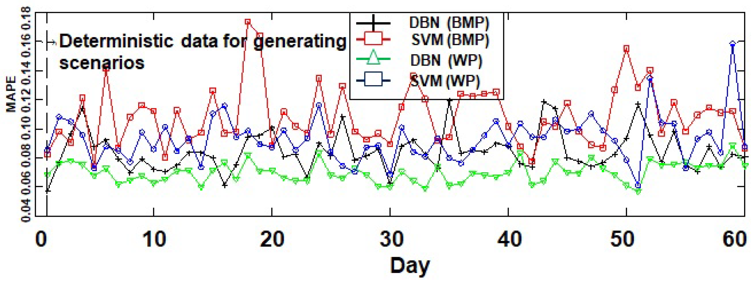
To validate the performance of the deterministic forecasting model based on DBN, the forecasting results of WP and BMP for two months are conducted, and SVM is used for comparison. The mean absolute percentage error (MAPE) [1] of forecasting results are shown in Figure 4. Our simulations reveal that the MAPE for BMP by exploiting the established DBN forecasting model ranges from 0.0571 to 0.1194 with an average of 0.0844 and that of SVM for BMP ranges from a minimum of 0.0743 to a maximum of 0.1732 with an average of 0.1086. Moreover, the average of DBN and SVM for WP are 0.06971 and 0.09283, respectively. The established forecasting model for BMP and WP is superior to the SVM with a higher average of MAPE. The greater accuracy of the established forecasting model is mainly because of the deep neural network structure that designs to appropriately optimize the inherent nonlinear features and hidden invariant architecture. Hence, the irregularity, dynamic complexity, and high non-linearity in BMP and WP data can be easily obtained.
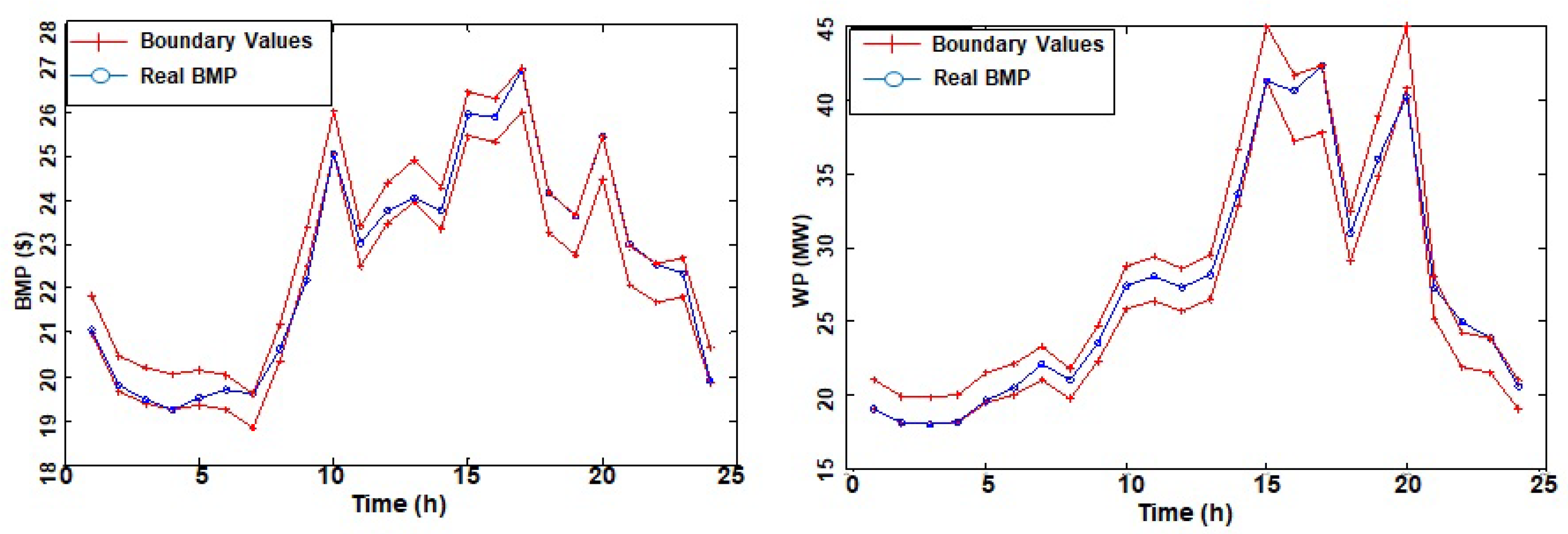
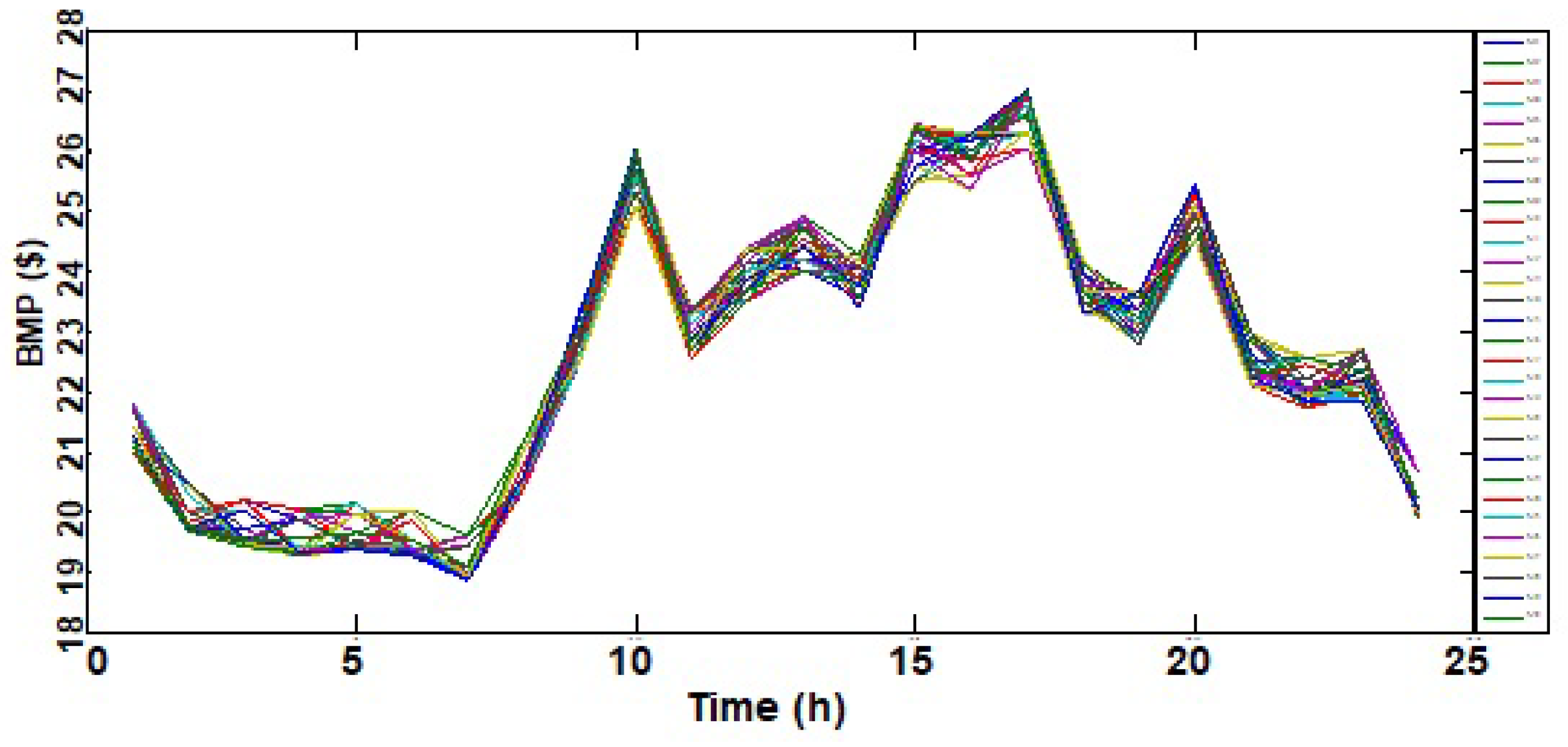
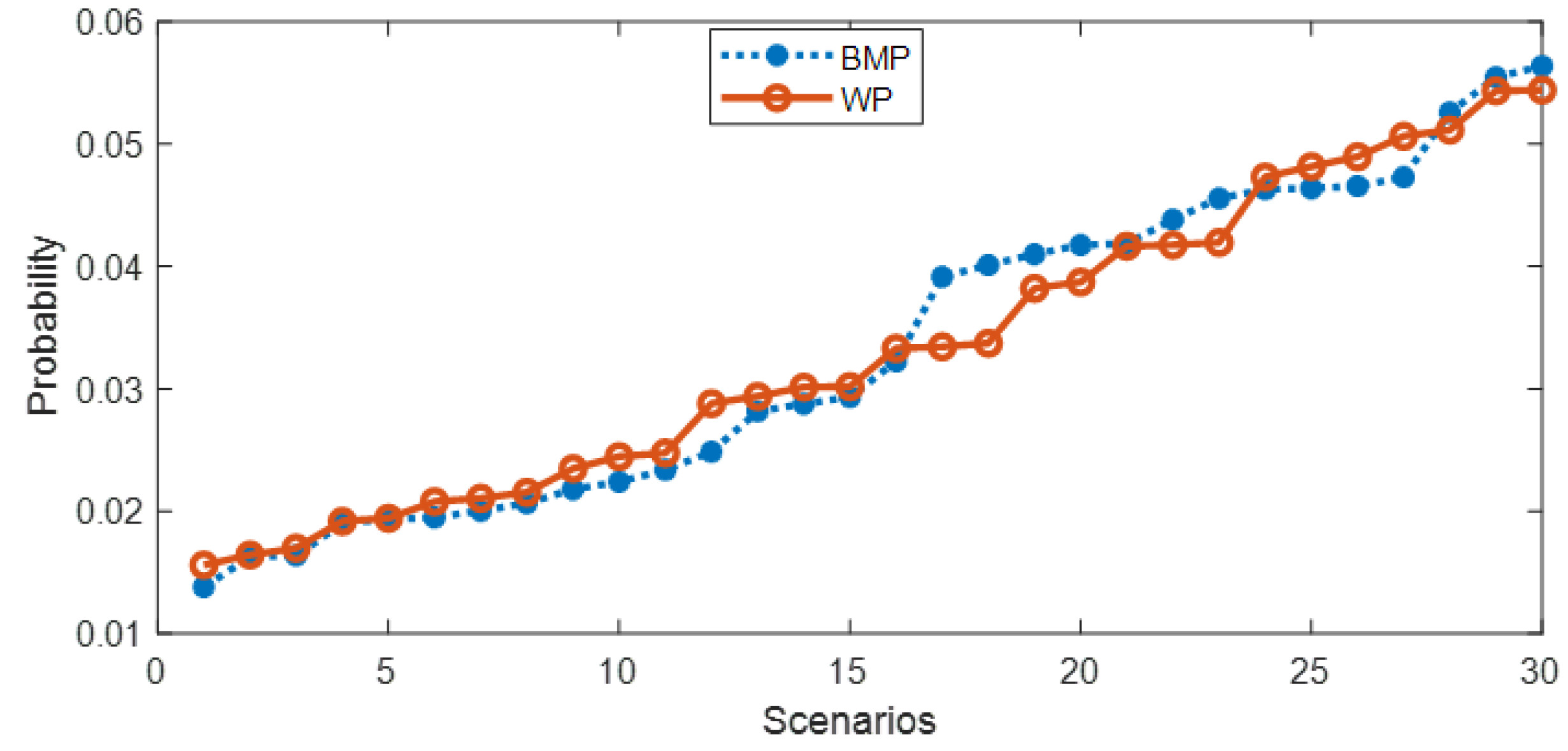
Generally, DBN-based deterministic forecasting for WP and BMP not directly applied to the optimal strategy of wind supplier, because DBN-based forecasting error could be only decreased but not be removed. Therefore, the QR is introduced in this paper to model the uncertainty related to WP and BMP. The trained dataset via an ensemble of deterministic forecasts will remain unchanged as before. And the BMP data on 1 September 2018, and the WP data on 1 September 2013 are individually selected and predicted to validate the performance. Figure 4 and Figure 5 graphically illustrate the constructed prediction interval (PI) with the predicted nominal interval confidence (PINC) 95% obtained by the predefined approach as well as the actual BMP data and WP data. It can be seen that the real data for WP and BMP are within the lower and upper bound, respectively, and their corresponding average coverage error (ACE) are individually 3.33% and 7.5%. This is because the errors acquired from the deterministic forecast for BMP have fewer uncertainties in comparison to WP data, as shown in Figure 5. Therefore, quantile regression ranging from 5% to 95% in 10% intervals are conducted by various confidence intervals and then generated every possible scenario based on the Monte Carlo simulation method [48,49]. Moreover, scenario reduction techniques [47] are also adopted to decrease to 30 scenarios simultaneously, because an enormous stochastic model would be less efficient, and a small stochastic model would not be reflecting the original scenarios. Figure 6 and Figure 7 depicts a set of 30 scenarios of WP and BMP for one day. Therefore, each scenario can describe the uncertainty and then be implemented in optimizing the BS of wind suppliers.

4.2.2. Optimal Performance Evaluation of an HPSOIFA

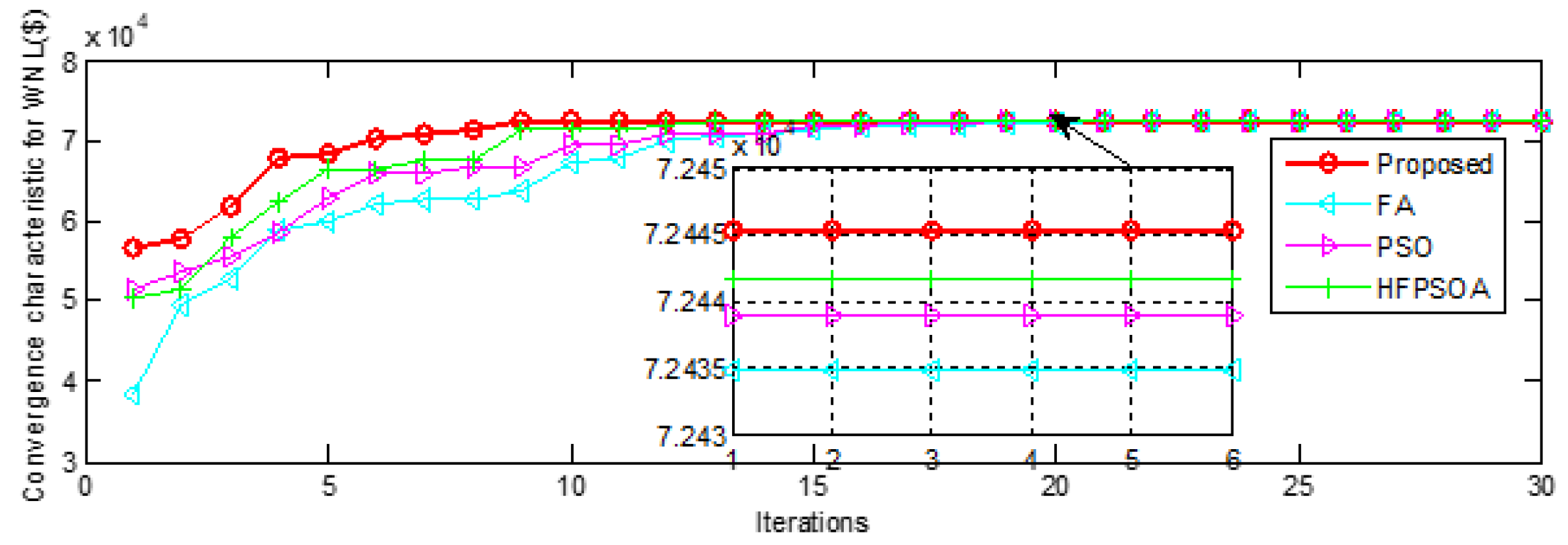
This subsection shows the effectiveness of the proposed HPSOIFA optimal algorithm. Sub-coalitions model S63 of a coalition (G1, G2, G3, G4, G5, and G6) expressing as complete cooperation was picked to exhibits the plausibility of the convergence performance. Additionally, the intelligent optimization algorithm with various problems represents different evolutionary performance, the optimization model without network loss (WNL) thus was used to validate the algorithm performance. Meanwhile, this performance is measured and evaluated by comparing the stability and convergence characteristics to hybrid firefly, PSO, and HFPSOA [29].
Table 1 shows the stability of the algorithm for WNL or CNL, while Figure 8 and Figure 9 shows the convergence characteristic. Figure 9 and Figure 10, shows that the proposed model has higher searching precision and fast convergence than PSO, FA, and HFPSOA. The mentioned scenarios are credited to the methods that are used in the blend of overall investigation with the PSO and local use with the IFA.
It is particularly important that the convergence attribute of the HFPSOA is slower compared to the given model. The chaotic sequence theory can keep it from starting at the local optimum. From the outcomes, it is evident that the proposed model has better results than PSO, FA, and HFPSOA, shown in Figure 9 and Figure 10. The algorithm performance is increased by using the characters of Halton initiation.
The performance of FA and the PSO will change with different parametric boundaries. Therefore, to confirm the solidness of the proposed calculation, the proposed calculation and differentiation techniques, such as FA, the PSO, and the HPSOFA are rehashed multiple times. For WNL, the combinations with HPSOIFA, FA, PSO, and HPSOFA are changed from U S D 72,442.65 to U S D 72,445.37, from U S D 72,429.67 to U S D 72,434.88, from U S D 72,432.29 to U S D 72,438.93, and from U S D 72,438.11 to U S D 72,441.67, individually, and their relating differences are 0.6821, 2.5027, 4.6050, and 1.1685, separately. For CNL, the proposed calculation moderately ( U S D 73,325.26) met with a fluctuation of 0.4213. The normal assembly of the FA, PSO, and HPSOFA are U S D 73,295.34 with a change of 3.9833, U S D 73,316.60 with a difference of 4.4631, and U S D 73,320.86 with a fluctuation of 0.7394. Thus, these outcomes likewise show from the point of view of the precision and solidness that the proposed calculation fundamentally beat the ordinary calculations.

4.3. Case 2: Investigations of CB Results

In this subsection, the issue due to loss in the network on the power suppliers’ BB is presented, and how to distribute the profits among the cooperative power suppliers. Then, the bi-layer CB model with different combinations for the wind energy suppliers is simulated and analyzed.

4.3.1. Impact Analysis on Network Loss and Profit Distribution by Shapley Value

The motivation behind this part is to explore the impact of network loss and how to disseminate benefits among helpful influence suppliers. To work on the conversation here, a totally agreeable offering model is chosen and examined at hour 8. For the above alliance, the trademark work an incentive as demonstrated in Figure 11 is determined in various sub-alliances Sc that is made out of S1, S2, S63, which decide the SV for every provider introduced in Table 2.
From Figure 6, the trademark works on incentive for completely cooperative offering at hour 8 displays their unanimity among WNL and CNL, as expected. This is on the grounds that network loss represents a little extent of the complete load. As can be found in Table 2, when 0.97, 1.60, 0.86, 1.40, 0.66, and 2.00 times of every provider marginal expense respectively, are finally chosen for BS dependent on WNL, the summation of Svz for power provider is USD 1991.5, and for CNL, when each power provider decide to offer at 1.53, 1.60, 1.32, 1.25, 1.49 and 1.98 times their minimal expense respectively, the summation of Svz for power provider are USD 2132.8. The outcomes show that the BS can change somewhat in light of the network loss. In any case, the benefits of the provider G4 are lower than zero in the two cases at hour 8. This does not accord to realities, which show that a totally agreeable offering may prompt disappointment.

4.3.2. Cooperative Bidding Results for a Wind Power Supplier

The purpose of this part is to search for the best cooperative BS for wind power suppliers. In general, cooperative power suppliers will be fixed within one day, when the sub-coalitions of CB are formed. We assumed that the wind power supplier (G1) collaborates with one conventional power supplier (Gc) against individual bidding members that are constituted of the remaining power suppliers. Therefore, a wind supplier exists five possible combinations (T1, T2, T3, T4, T5), which are (G1, G2), G3, G4, G5, G6, (G1,G3), G2, G4, G5, G6, (G1,G4), G2, G4, G5, G6, (G1,G5), G2, G4, G5, G6 and (G1,G6), G2, G4, G5, G6, respectively. Moreover, the SV is exploited to the profit distribution for cooperative suppliers, as illustrated above. Meanwhile, the individual bidding profits for six power suppliers can be obtained by Equation (1) (e.g., cooperative power supplier is not existing) to calculate the additional cooperative profits. Based on the situation above, different market profits of G1 suppliers at a different time under completely non-CB for six power suppliers are carried out and the results are presented in Figure 12. Furthermore, Table 3 presents the power suppliers’ profits of five combinations in different bidding types.
From Figure 13, it can be observed that the profits of the wind energy supplier in the day-ahead market stay almost the same. This result is due to the market power where the BM does not have great enough to influence the day-ahead LMP. The total profits of the wind energy suppliers have shown a wide range of fluctuation from 14 h to 20 h. This is due to the high production of wind energy compared with other times. As shown in Figure 11, the profits in the BM have increased from 14 h to 20 h. Statistical results shown form Table 3 that the profits of the wind energy suppliers for each combination are varied from U S D 11,389 to U S D 10,238, from U S D 11,389 to U S D 11,956, from U S D 11,389 to U S D 9685, from U S D 11,389 to U S D 11,772, and from U S D 11,389 to U S D 14,792, respectively, with the corresponding extra profits U S D −1976, U S D 567, U S D −1704, U S D 383, and U S D 3403. The cooperative profits of conventional suppliers for each combination are U S D 15,861 with an extra profit of U S D 5778, U S D 9140 with an extra profit of U S D 1810, U S D 2556 with an extra profit of U S D −1272, U S D 9335 with an extra profit of U S D 492, and U S D 22,565 with an extra profit of U S D 2998. These data suggest that the wind energy supplier may be more active and cooperative with conventional power suppliers (G3, G5, or G6). Therefore, we can summarize that CB for wind energy suppliers may improve its profits. To some extent, this is due to the CB can reduce its congestion and non-cooperative power suppliers’ profits.

5. Conclusions

A novel bidding model incorporating NL and coalition formation based on the WP and BMP uncertainty quantification has been newly proposed in this paper, to improve the wind energy suppliers’ benefit. Then, a solver, including an evolutionary game approach (EGA), hybrid PSO, and an improved FA is proposed to efficiently tackle the bidding challenges. Moreover, the combination of a deep belief network (DBN) forecasting framework and quantile regression (QR) is employed to reduce the wind energy bidding uncertainty. Finally, the distribution of the cooperative benefits is exploited by Shapley value (SV). The bidding model and proposed algorithms under a modified IEEE 30-bus system have been proved to be feasible and effective.
The statistical results demonstrate that a solver can obtain a wonderful solution when compared with the standard one. It is because of the novel BS that has adopted overall exploration with PSO, nearby exploitation with FA, and chaotic-sequence-based approach. At the same time, the result shows that a predictor can reduce the uncertainty of wind production and BM price when compared to the routine method. This is because the inner structures and features can primly be extracted using a deep belief algorithm. In the end, the numerical results from the CB exhibit that the CB of the wind energy suppliers may increase their profit; however, there is a chance of collation collapse. The influence of the network loss (NL) on the power suppliers’ bidding behavior (BB) is also investigated. The established model and the proposed algorithms offer significant benefits for the wind energy suppliers’ bidding.
There are some important considerations which have not been included in this research, such as (1) the consideration of the demand-side bidding in the proposed model, as it may also affect the market equilibrium; and (2) a balance between the simulation accuracy and computational efficiency of the methods, which may a concern for large-scale power system simulation. Hence, the future work will consider implementing the demand-side bidding and accuracy-efficiency mapping of the model to test and demonstrate its suitability for a wide range of scenarios.

Author Contributions

Conceptualization, R.Z., S.A. (Saddam Aziz) and M.U.F.; methodology and formal analysis, R.Z., S.A. (Saddam Aziz); software, data curation and validation, R.Z.; writing—original draft preparation, K.N.H., N.M., S.A. (Saddam Aziz) and N.I.; writing—review and editing, R.Z., S.A. (Sadiq Ahmad), M.U.F., K.N.H., S.A. (Saddam Aziz) and N.M.; visualization, R.Z., S.A. (Sadiq Ahmad); supervision, S.A. (Saddam Aziz); project administration, S.A. (Saddam Aziz), R.Z.; funding acquisition, S.A. (Saddam Aziz), N.M. All authors have read and agreed to the published version of the manuscript.

Funding

This work is supported by Foundation of Shenzhen Science and Technology Committee, worth of project funding by Govt of China.

Conflicts of Interest

The authors declare no conflict of interest.

Abbreviations

The following abbreviations are used in this manuscript:
LMPlocational marginal price
WPwind production
BMbalancing market
BMPbalancing market price
BSbidding strategy
EGAevolutionary game approach
PSOparticle swarm optimization
FAfirefly algorithm
HPSOIFAhybrid particle swarm optimization and improved firefly algorithm
QRquantile regression
SVShapley value
ISOindependent system operator’s
DBNdeep belief network

References

  1. Wang, H.; Liu, Y.; Zhou, B.; Li, C.; Cao, G.; Voropai, N.; Barakhtenko, E. Taxonomy research of artificial intelligence for deterministic solar power forecasting. Energy Convers. Manag. 2020, 214, 112909. [Google Scholar] [CrossRef]
  2. Aziz, S.; Wang, H.; Liu, Y.; Peng, J.; Jiang, H. Variable universe fuzzy logic-based hybrid LFC control with real-time implementation. IEEE Access 2019, 7, 25535–25546. [Google Scholar] [CrossRef]
  3. Zhang, H.; Liu, X.; Ji, H.; Hou, Z.; Fan, L. Multi-Agent-Based Data-Driven Distributed Adaptive Cooperative Control in Urban Traffic Signal Timing. Energies 2019, 12, 1402. [Google Scholar] [CrossRef] [Green Version]
  4. Yang, W.; Wang, M.; Aziz, S.; Kharal, A.Y. Magnitude-Reshaping Strategy for Harmonic Suppression of VSG-Based Inverter Under Weak Grid. IEEE Access 2020, 8, 184399–184413. [Google Scholar] [CrossRef]
  5. Baringo, L.; Conejo, A.J. Strategic Offering for a Wind Power Producer. IEEE Trans. Power Syst. 2013, 28, 4645–4654. [Google Scholar] [CrossRef]
  6. The Gansu Power Trading Center Official Website. Available online: https://pmos.gs.sgcc.com.cn (accessed on 14 September 2020).
  7. The ERCOT Website. Available online: https://www.tklaw.com/services/ercot (accessed on 21 September 2020).
  8. The PJM Official Website. Available online: https://www.pjm.com/markets-and-operations/data-dictionary.aspx/ (accessed on 11 September 2020).
  9. Zugno, M.; Morales, J.M.; Pinson, P.; Madsen, H. Pool Strategy of a Price-Maker Wind Power Producer. IEEE Trans. Power Syst. 2013, 28, 3440–3450. [Google Scholar] [CrossRef] [Green Version]
  10. Xiao, Y.; Wang, X.; Wang, X.; Dang, C.; Lu, M. Behavior analysis of wind power producer in electricity market. Appl. Energy 2016, 171, 325–335. [Google Scholar] [CrossRef]
  11. de la Nieta, A.A.S.; Contreras, J.; Muñoz, J.I.; O’Malley, M. Modeling the Impact of a Wind Power Producer as a Price-Maker. IEEE Trans. Power Syst. 2014, 29, 2723–2732. [Google Scholar] [CrossRef]
  12. Li, Y.; Xue, W.; Wu, T.; Wang, H.; Zhou, B.; Aziz, S.; He, Y. Intrusion detection of cyber physical energy system based on multivariate ensemble classification. Energy 2021, 218, 119505. [Google Scholar] [CrossRef]
  13. Banaei, M.; Buygi, M.O.; Zareipour, H. Impacts of Strategic Bidding of Wind Power Producers on Electricity Markets. IEEE Trans. Power Syst. 2016, 31, 4544–4553. [Google Scholar] [CrossRef]
  14. Wang, Y.; Wang, D.; Zhang, H.; Zhang, K. Optimal Bidding of Price-Maker Retailers With Demand Price Quota Curves Under Price Uncertainty. IEEE Access 2020, 8, 120746–120756. [Google Scholar] [CrossRef]
  15. Wang, J.; Zhou, Z.; Botterud, A. An evolutionary game approach to analyzing bidding strategies in electricity markets with elastic demand. Energy 2011, 36, 3459–3467. [Google Scholar] [CrossRef]
  16. Shafie-Khah, M.; Heydarian-Forushani, E.; Golshan, M.E.H.; Moghaddam, M.P.; Sheikh-El-Eslami, M.K.; Catalao, J.P.S. Strategic Offering for a Price-Maker Wind Power Producer in Oligopoly Markets Considering Demand Response Exchange. IEEE Trans. Ind. Inform. 2015, 11, 1542–1553. [Google Scholar] [CrossRef]
  17. Dai, T.; Wei, Q. Optimal Bidding Strategy of a Strategic Wind Power Producer in the Short-Term Market. IEEE Trans. Sustain. Energy 2017, 6, 707–719. [Google Scholar] [CrossRef]
  18. Stanford Encyclopedia of Philosophy. Available online: http://plato.stanford.edu/entries/game-evolutionary/ (accessed on 6 September 2019).
  19. Wang, D.; Li, B. Behavioral Selection Strategies of Members of Enterprise Community of Practice—An Evolutionary Game Theory Approach to the Knowledge Creation Process. IEEE Access 2020, 8, 153322–153333. [Google Scholar] [CrossRef]
  20. Wen, X.; Peng, J.; Aziz, S.; Jiang, H. PCC Voltage Compensation Scheme of MMC-MTDC System for Transient Stability Enhancement Under Communication Delay. IEEE Access 2020, 8, 187713–187720. [Google Scholar] [CrossRef]
  21. Niknam, T.; Sharifinia, S.; Azizipanah-Abarghooee, R. A new enhanced bat-inspired algorithm for finding linear supply function equilibrium of GENCOs in the competitive electricity market. Energy Convers. Manag. 2013, 76, 1015–1028. [Google Scholar] [CrossRef]
  22. Peng, X.; Tao, X. Cooperative game of electricity retailers in China’s spot electricity market. Energy 2018, 145, 152–170. [Google Scholar] [CrossRef]
  23. Soliman, M.A.; Hasanien, H.M.; Azazi, H.Z.; El-Kholy, E.E.; Mahmoud, S.A. Hybrid ANFIS-GA-based control scheme for performance enhancement of a grid-connected wind generator. IET Renew. Power Gener. 2018, 12, 832–843. [Google Scholar] [CrossRef]
  24. Li, T.; Shahidehpour, M. Strategic Bidding of Transmission-Constrained GENCOs with Incomplete Information. IEEE Trans-Actions Power Syst. 2005, 20, 437–447. [Google Scholar] [CrossRef]
  25. Litvinov, E.; Zheng, T.; Rosenwald, G.; Shamsollahi, P. Marginal Loss Modeling in LMP Calculation. IEEE Trans. Power Syst. 2004, 19, 880–888. [Google Scholar] [CrossRef]
  26. Stern, A.; Tettenhorst, A. Hodge decomposition and the Shapley value of a cooperative game. Games Econ. Behav. 2019, 113, 186–198. [Google Scholar] [CrossRef] [Green Version]
  27. Ma, Z.; Guo, S.; Xu, G.; Aziz, S. Meta Learning-Based Hybrid Ensemble Approach for Short-Term Wind Speed Forecasting. IEEE Access 2020, 8, 172859–172868. [Google Scholar] [CrossRef]
  28. Jana, B.; Mitra, S.; Acharyya, S. Repository and Mutation based Particle Swarm Optimization (RMPSO): A new PSO variant applied to reconstruction of Gene Regulatory Network. Appl. Soft Comput. 2019, 74, 330–355. [Google Scholar] [CrossRef]
  29. Aydilek, İ.B. A Hybrid Firefly and Particle Swarm Optimization Algorithm for Computationally Expensive Numerical Problems. Appl. Soft Comput. 2018, 66, S1568494618300. [Google Scholar] [CrossRef]
  30. Ruan, J.; Wang, H.; Aziz, S.; Wang, G.; Zhou, B.; Fu, X. Interval state estimation based defense mechanism against cyber attack on power systems. In Proceedings of the 2017 IEEE Conference on Energy Internet and Energy System Integration (EI2), Beijing, China, 26–28 November 2017; pp. 1–5. [Google Scholar]
  31. Kiran, M.S.; Gunduz, M. A recombination-based hybridization of particle swarm optimization and artificial bee colony al-gorithm for continuous optimization problems. Appl. Soft Comput. 2013, 13, 2188–2203. [Google Scholar] [CrossRef]
  32. Aziz, S.; Peng, J.; Wang, H.; Jiang, H. ADMM-Based Distributed Optimization of Hybrid MTDC-AC Grid for Determining Smooth Operation Point. IEEE Access 2019, 7, 74238–74247. [Google Scholar] [CrossRef]
  33. Yang, X.S.; He, X. Firefly Algorithm: Recent Advances and Applications. Int. J. Swarm Intell. 2013, 1, 36–50. [Google Scholar] [CrossRef] [Green Version]
  34. Wang, H.; Cai, R.; Zhou, B.; Aziz, S.; Qin, B.; Voropai, N.; Gan, L.; Barakhtenko, E. Solar irradiance forecasting based on direct explainable neural network. Energy Convers. Manag. 2020, 226, 113487. [Google Scholar] [CrossRef]
  35. Wang, H.; Wang, W.; Zhou, X.; Sun, H.; Zhao, J.; Yu, X.; Cui, Z. Firefly algorithm with neighborhood attraction. Inform. Sci. 2017, 382–383, 374–879. [Google Scholar] [CrossRef]
  36. Caponetto, R.; Fortuna, L.; Fazzino, S.; Xibilia, M. Chaotic sequences to improve the performance of evolutionary algorithms. IEEE Trans. Evol. Comput. 2003, 7, 289–304. [Google Scholar] [CrossRef]
  37. Liu, Y.; Jiang, H.; Peng, J.; Aziz, S. A Grouping-Based Frequency Support Scheme for Wind Farm Under Cyber Uncertainty. IEEE Access 2020, 8, 178044–178054. [Google Scholar] [CrossRef]
  38. Xiang, L.; Deng, Z.; Hu, A. Forecasting Short-Term Wind Speed Based on IEWT-LSSVM Model Optimized by Bird Swarm Algorithm. IEEE Access 2019, 7, 59333–59345. [Google Scholar] [CrossRef]
  39. Marir, N.; Wang, H.; Feng, G.; Li, B.; Jia, M. Distributed Abnormal Behavior Detection Approach Based on Deep Belief Network and Ensemble SVM Using Spark. IEEE Access 2018, 6, 59657–59671. [Google Scholar] [CrossRef]
  40. Awange, J.L.; Paláncz, B.; Lewis, R.H.; Völgyesi, L. Quantile Regression; Springer: Cham, Switzerland; New York, NY, USA, 2018. [Google Scholar]
  41. Le Roux, N.; Bengio, Y. Representational Power of Restricted Boltzmann Machines and Deep Belief Networks. Neural Comput. 2008, 20, 1631–1649. [Google Scholar] [CrossRef] [PubMed]
  42. Hinton, G.E.; Osindero, S.; Teh, Y.W. A Fast Learning Algorithm for Deep Belief Nets. Neural Comput. 2006, 18, 1527–1554. [Google Scholar] [CrossRef]
  43. Lei, Z.; Wang, H.; Wen, X.; Meng, A.; Aziz, S. Wind Power Forecasting Based on Echo State Network. In Proceedings of the 2019 IEEE Sustainable Power and Energy Conference (iSPEC), Beijing, China, 21–23 November 2019; pp. 268–272. [Google Scholar]
  44. Sun, S.; Fu, J.; Wei, L.; Li, A. Multi-Objective Optimal Dispatching for a Grid-Connected Micro-Grid Considering Wind Power Forecasting Probability. IEEE Access 2020, 8, 46981–46997. [Google Scholar] [CrossRef]
  45. Zhang, R.; Li, G.; Ma, Z. A Deep Learning Based Hybrid Framework for Day-Ahead Electricity Price Forecasting. IEEE Access 2020, 8, 143423–143436. [Google Scholar] [CrossRef]
  46. Shahidehpour, M.; Wang, Y. Appendix C: IEEE-30 Bus System Data. In Communication and Control in Electric Power Systems; Wiley-IEEE Press: Hoboken, NJ, USA, 2005. [Google Scholar]
  47. Wang, H.; Zhang, R.; Peng, J.; Wang, G.; Liu, Y.; Jiang, H.; Liu, W. GPNBI-inspired MOSFA for Pareto operation optimization of integrated energy system. Energy Convers. Manag. 2017, 151, 524–537. [Google Scholar] [CrossRef]
  48. Camal, S.; Teng, F.; Michiorri, A.; Kariniotakis, G.; Badesa, L. Scenario generation of aggregated Wind, Photovoltaics and small Hydro production for power systems applications. Appl. Energy 2019, 242, 1396–1406. [Google Scholar] [CrossRef] [Green Version]
  49. Li, T.; Shahidehpour, M.; Li, Z. Risk-Constrained Bidding Strategy With Stochastic Unit Commitment. IEEE Trans. Power Syst. 2007, 22, 449–458. [Google Scholar] [CrossRef]
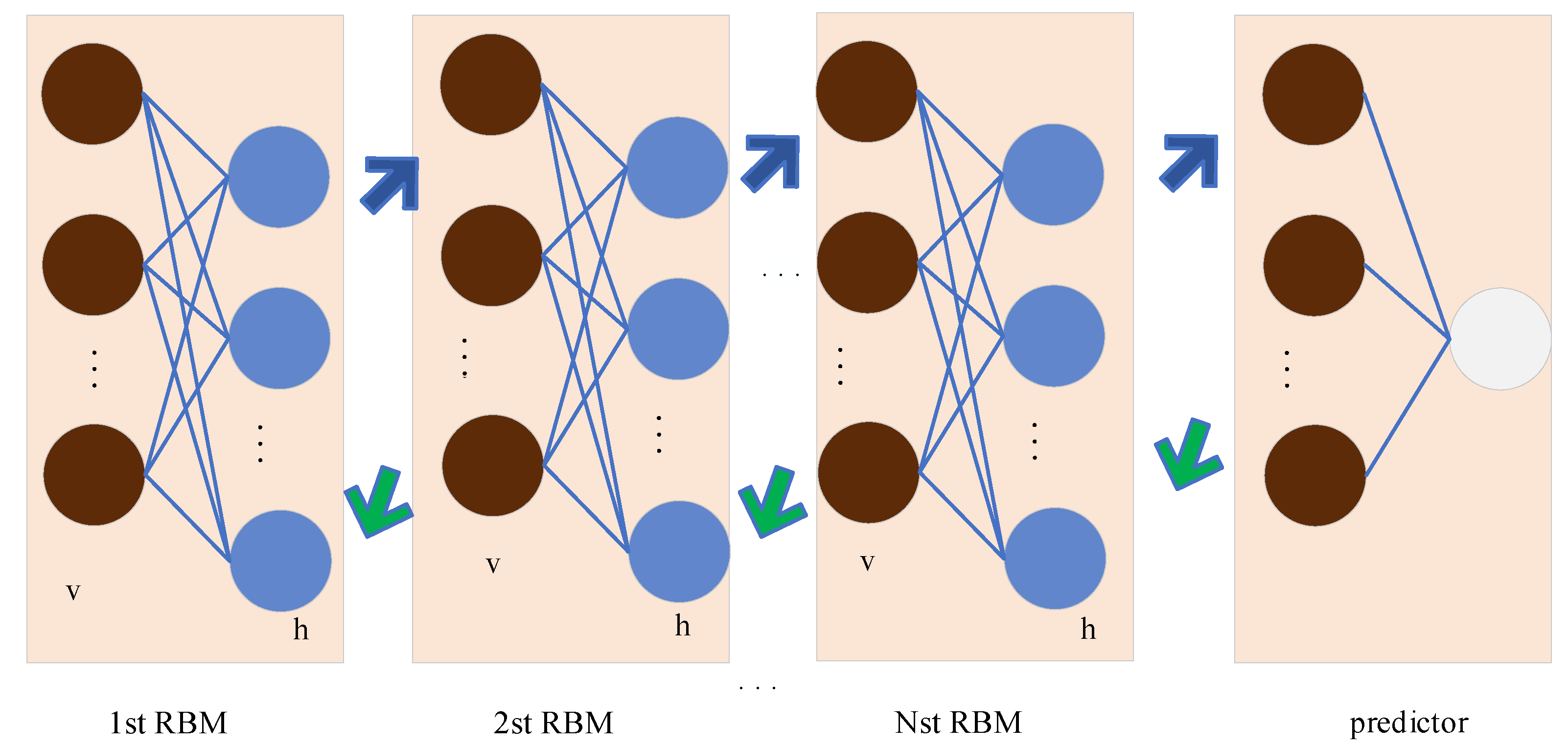
Figure 1. The Deep Belief Network (DBN) architecture.
Energies 14 03059 g001
Figure 2. The restricted Boltzmann machine (RBM) architecture.
Energies 14 03059 g002
Figure 3. Flowchart of the wind energy suppliers’ market bidding algorithm.
Energies 14 03059 g003
Figure 4. The MAPE statistics of WP and BMP.
Energies 14 03059 g004
Figure 5. BMP and WP of PIs with PINC 95%.
Energies 14 03059 g005
Figure 6. The BMP with 30 alternative scenarios.
Energies 14 03059 g006
Figure 7. The WP with 30 alternative scenarios.
Energies 14 03059 g007
Figure 8. The probability of BMP and WP for 30 alternative scenarios.
Energies 14 03059 g008
Figure 9. The convergence characteristic for the WNL.
Energies 14 03059 g009
Figure 10. The convergence characteristic for the CNL.
Energies 14 03059 g010
Figure 11. The characteristic function value of v(Sc) for completely CB at hour 8.
Energies 14 03059 g011
Figure 12. Different market profits of G1 supplier under completely individual bidding.
Energies 14 03059 g012
Figure 13. (a) The profit of wind power supplier under the coalition. (b) The profit of cooperative power suppliers under the coalition.
Energies 14 03059 g013
Table 1. Statistical convergence metrics of various algorithms.
KindAlgorithmsBest (USD)Worst (USD)Mean (USD)Var.
WNLProposed72,445.3772,442.6572,444.890.6821
FA72,434.8872,429.6772,432.992.5027
PSO72,438.9372,432.2972,435.614.6050
HFPSOA72,441.6772,438.1172,439.891.1685
CNLProposed73,326.3873,324.2873,325.260.4213
FA73,298.7973,292.3273,295.343.9833
PSO73,320.2573,313.4173,316.604.4631
HFPSOA73,322.3473,319.5673,320.860.7394
Table 2. Optimal BS and SV of each power provider for completely CB at hour 8.
TypeNoG1G2G3G4 G5G6
WNLK0.971.600.861.400.662.00
Sv(USD)611.964.8474.0−1066.1895.51011.3
CNLk1.531.601.321.251.491.98
Sv (USD)440.53582.4243.6−888.4682.71072
Table 3. Comparison of profits with and without considering coalitions.
CombinationsT1(USD)T2(USD)T3(USD)T4(USD)T4(USD)
Profit without coalition for G111,38911,38911,38911,38911,389
Profit considering coalition for G110,23811,956968511,77214,792
Extra profit for G1−1976567−17043833403
Profit without coalition for Gc10,08373303828884319,567
Profit considering coalition for Gc15,86191402556933522,565
Extra profit for Gc57781810−12724922998
Publisher’s Note: MDPI stays neutral with regard to jurisdictional claims in published maps and institutional affiliations.