Use of Concentric Hele-Shaw Cell for the Study of Displacement Flow and Interface Tracking in Primary Cementing


Abstract
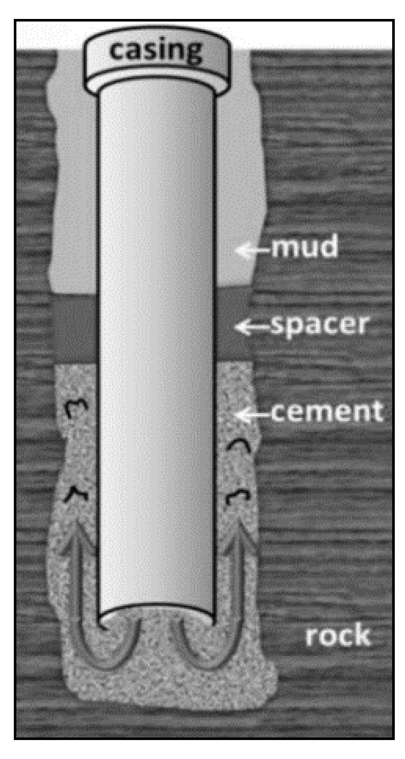
1. Introduction
2. Experimental Description
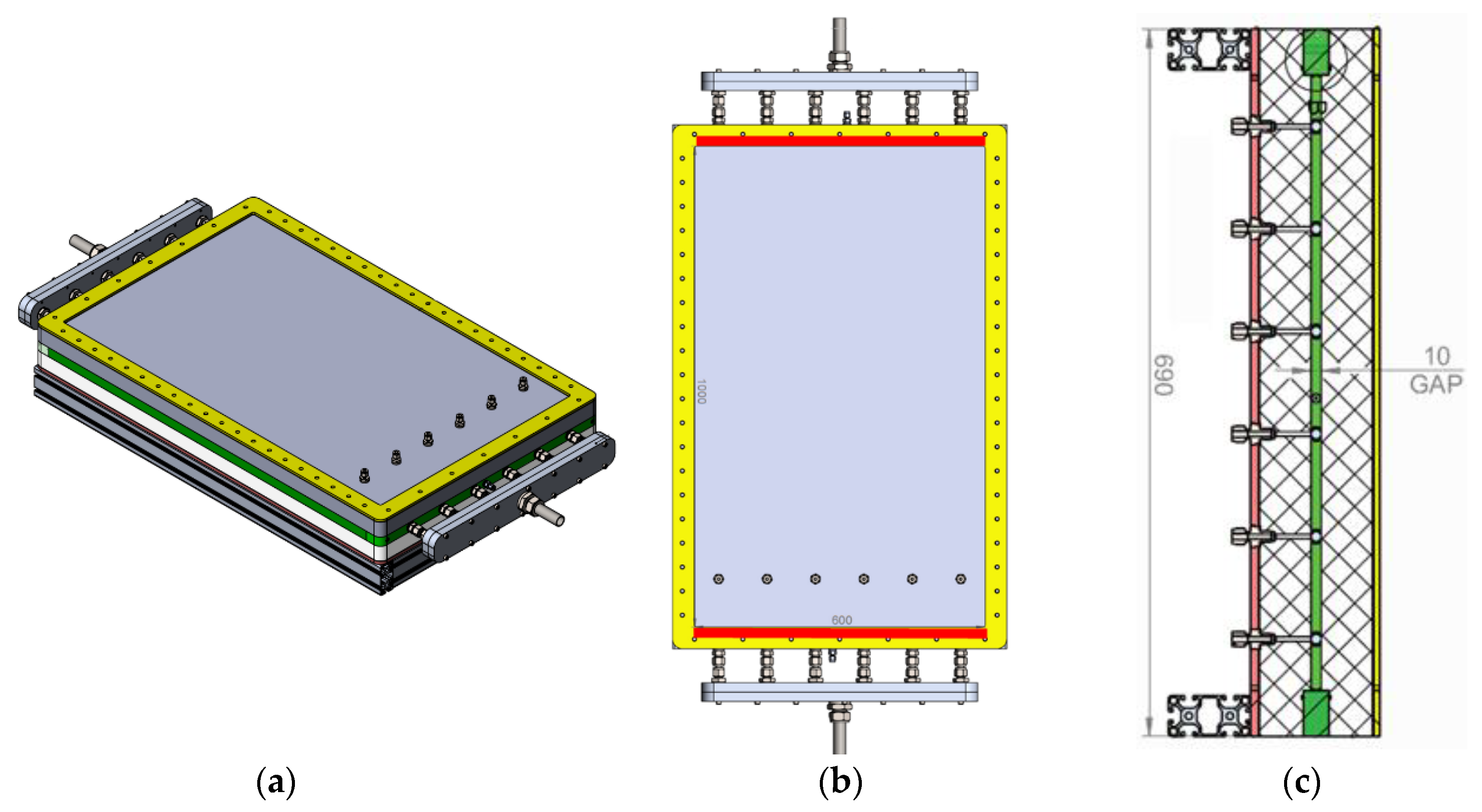
2.1. Experimental Design
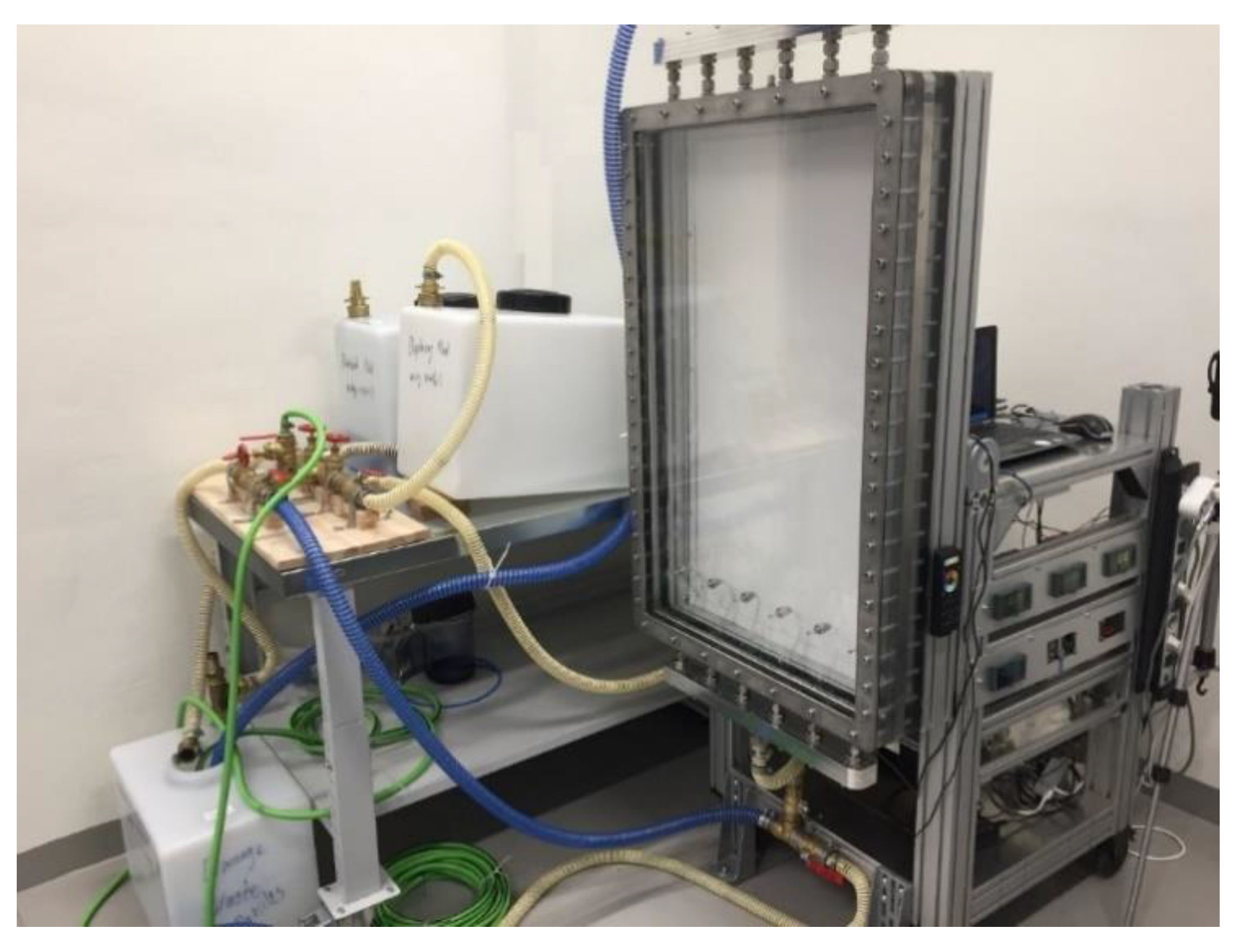
2.2. Experimental Set-Up and Procedure
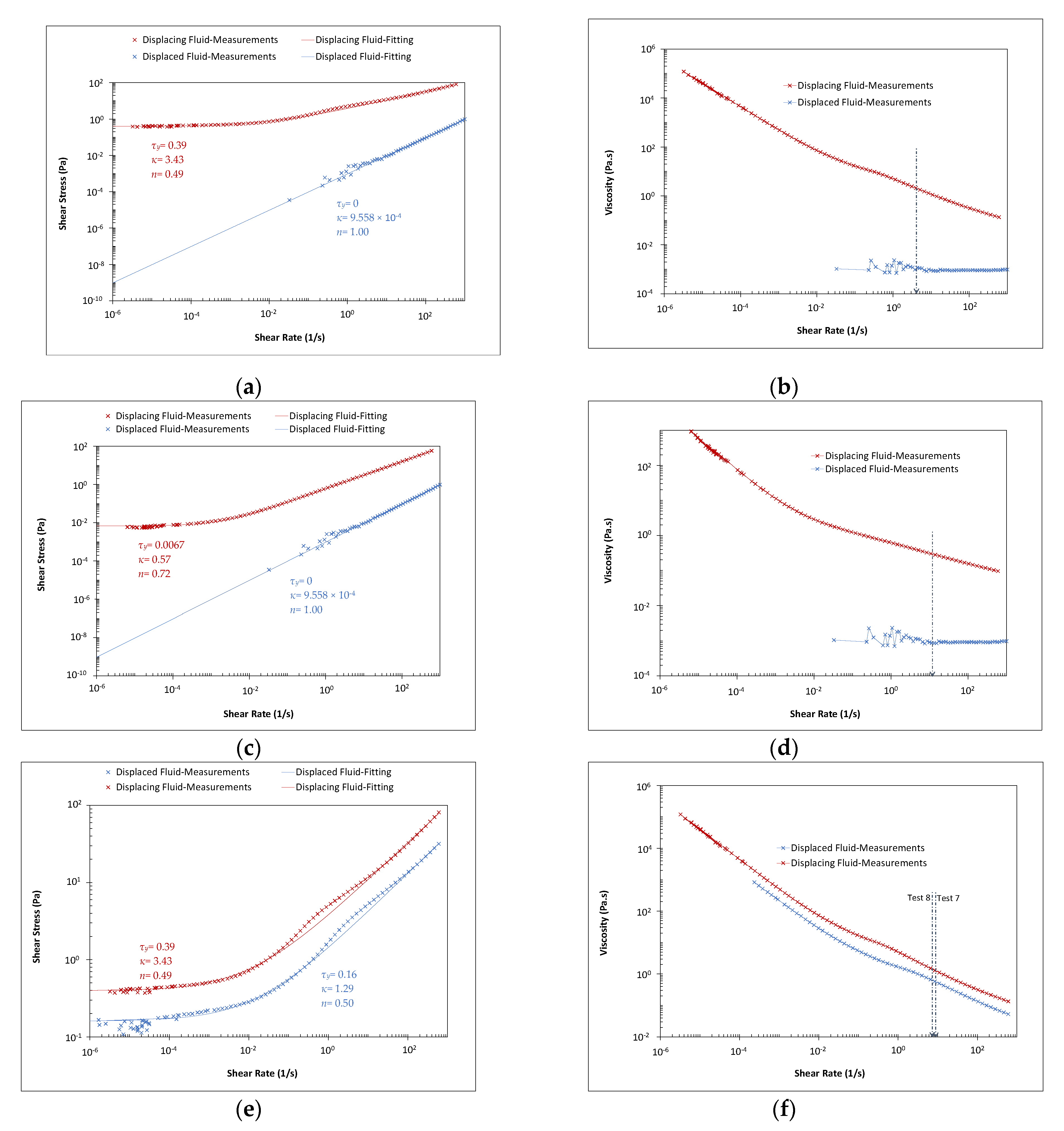
2.3. Fluid Preparation and Property Measurement
2.4. Experimental Overview
3. Experimental Results and Discussion
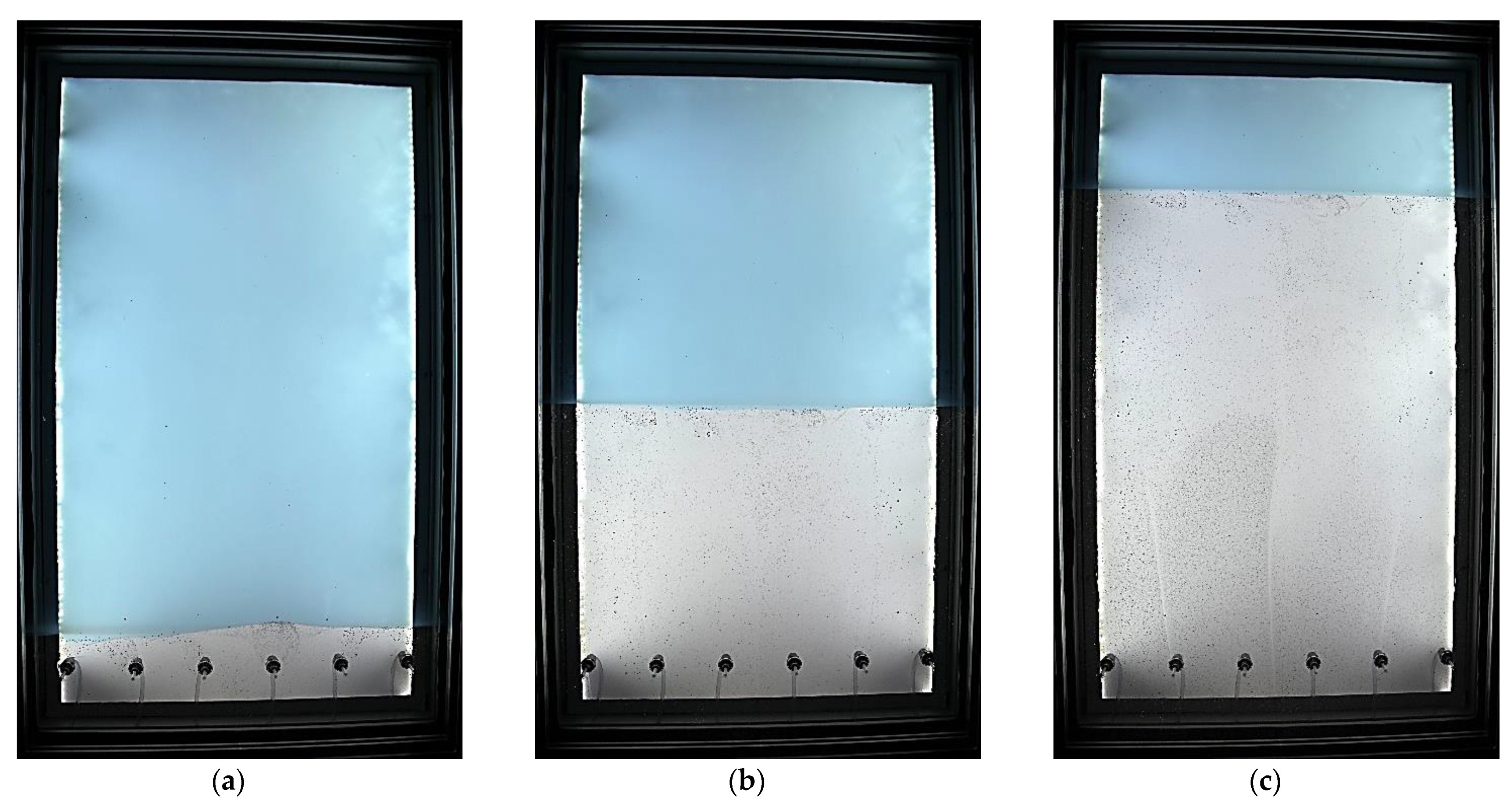
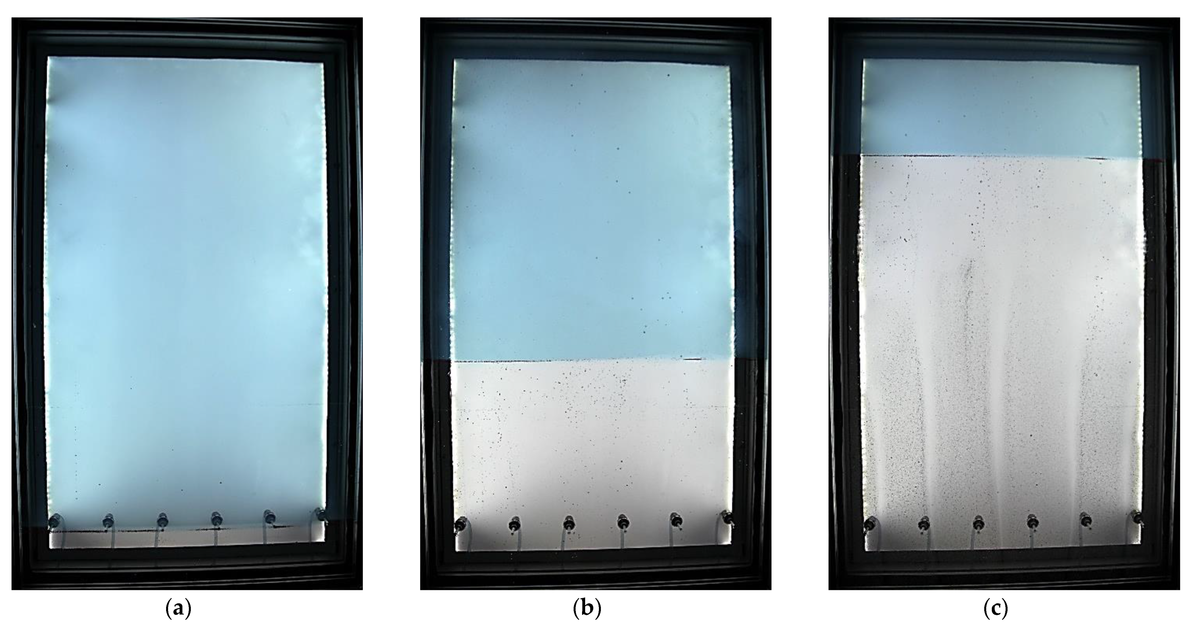
3.1. Stable Displacement
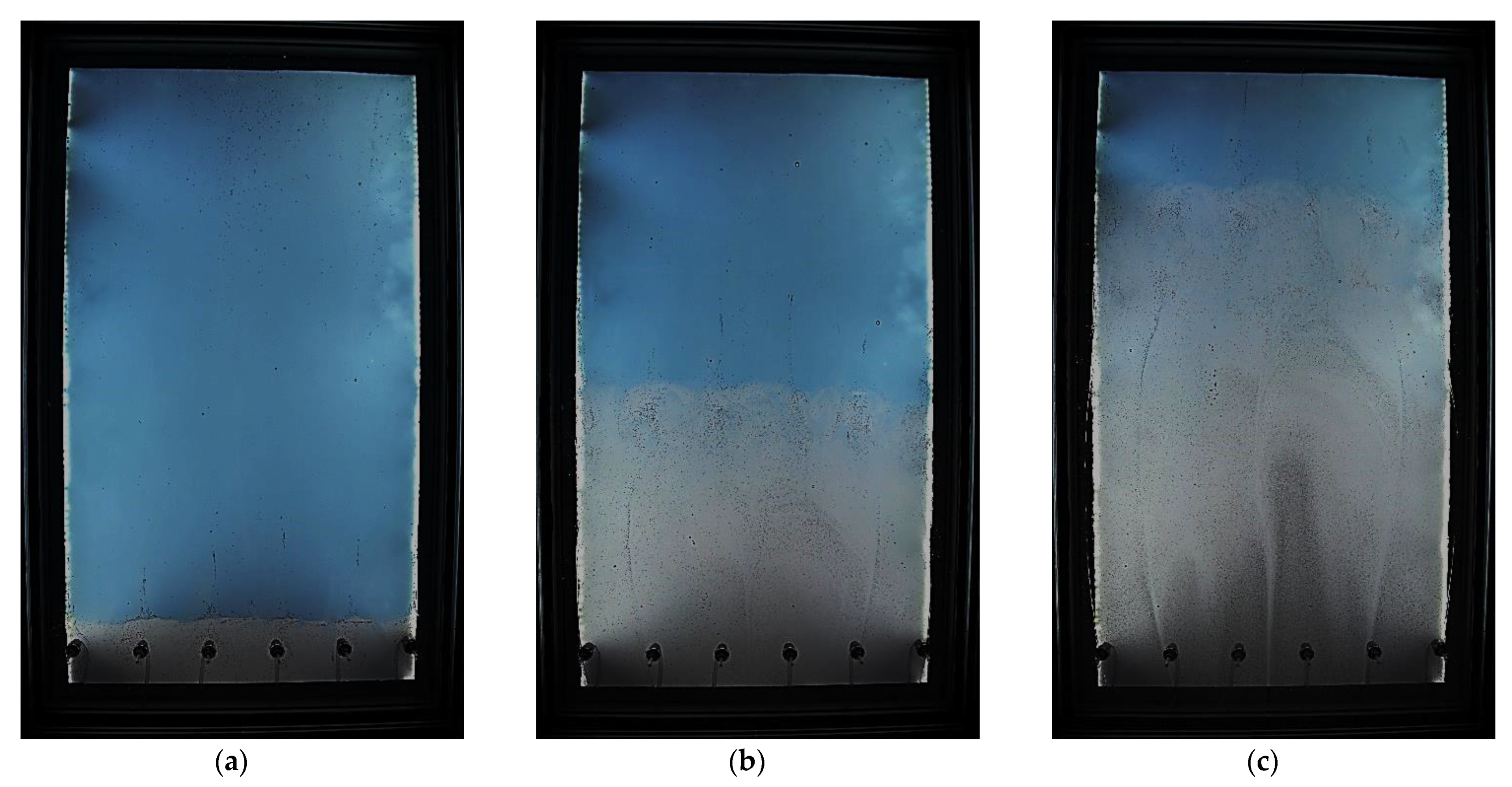
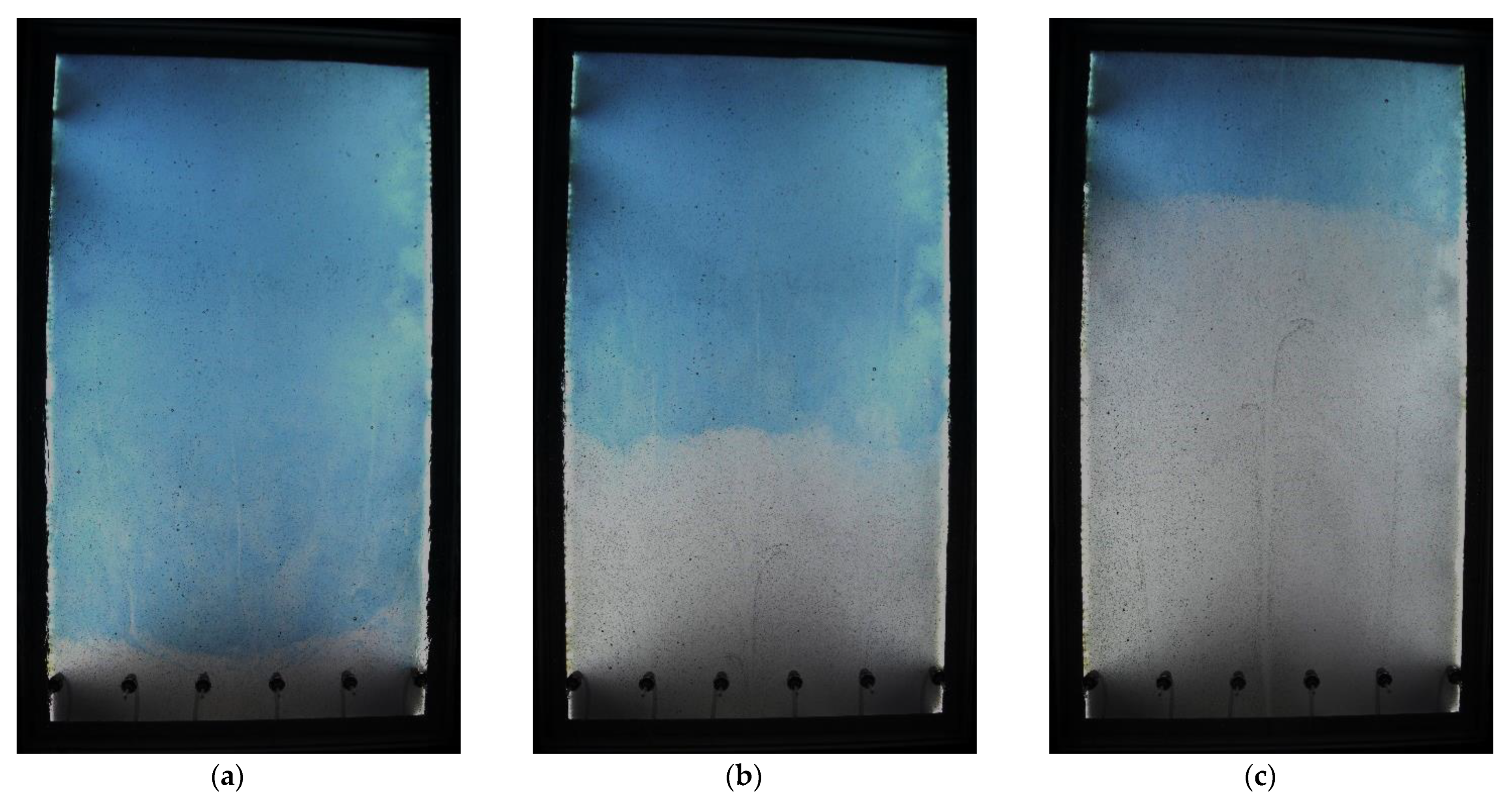
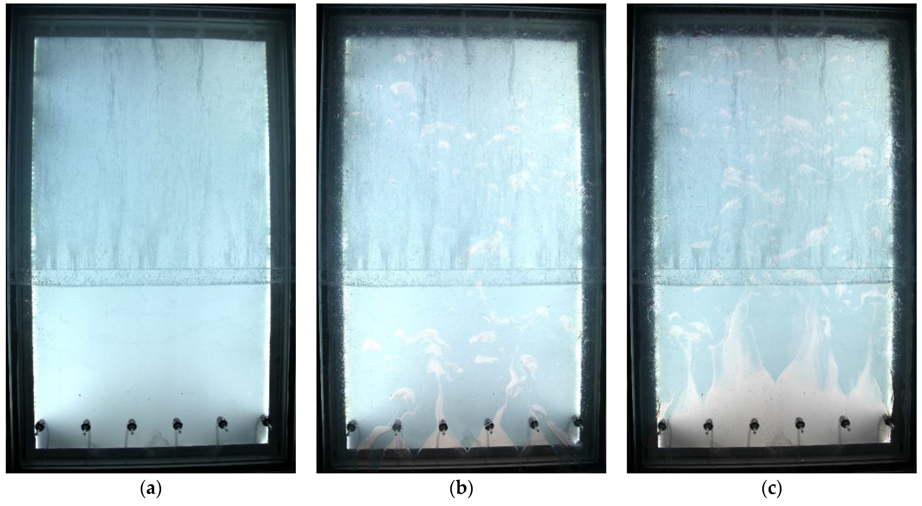
3.2. Unstable Displacement
4. Conclusions
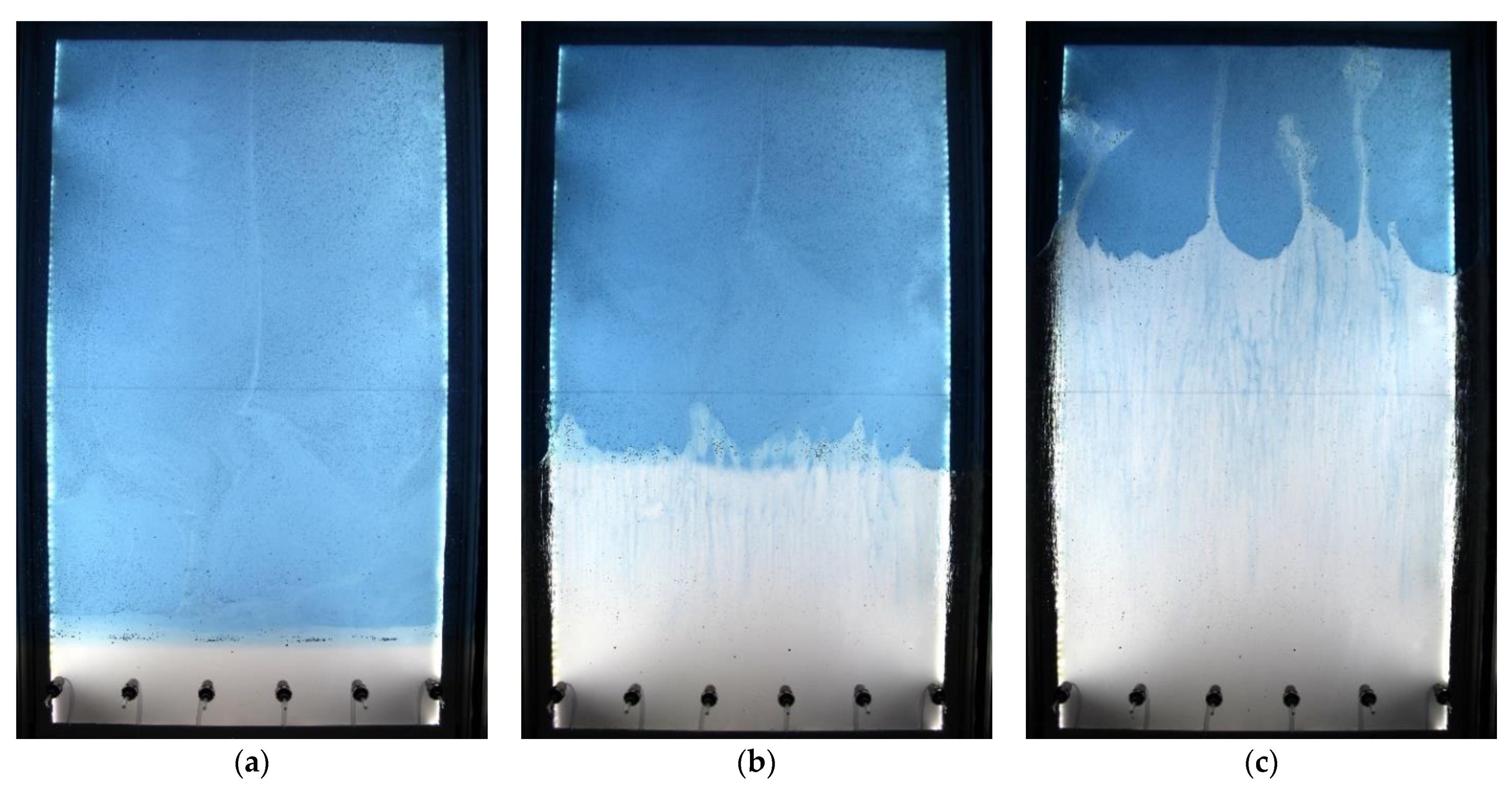
- Our qualitative results confirm that while the vertical displacement of a fluid by another with higher density and viscosity is stable with a flat interface, the displacement of a fluid with another one with lower equivalent viscosity causes viscous fingering and unstable displacement. Viscous fingering increases by increasing the displacement flow rate and the difference of equivalent viscosities of the two fluids. Moreover, displacement of a fluid with another one with lower density causes bubble flow and extremely poor displacement.
- Bypassing of pockets of the displaced yield-stress fluid by the displacing fluid has been another observed phenomenon in the experiments. This bypassing has also been observed in stable displacement cases and increases by decreasing displacement efficiency and increasing viscous fingering. Displacement of a yield-stress fluid by another yield-stress fluid decreases the bypassing of the pockets of yield-stress displaced fluid, and its possibility is decreased when the two fluids have close yield-stresses.
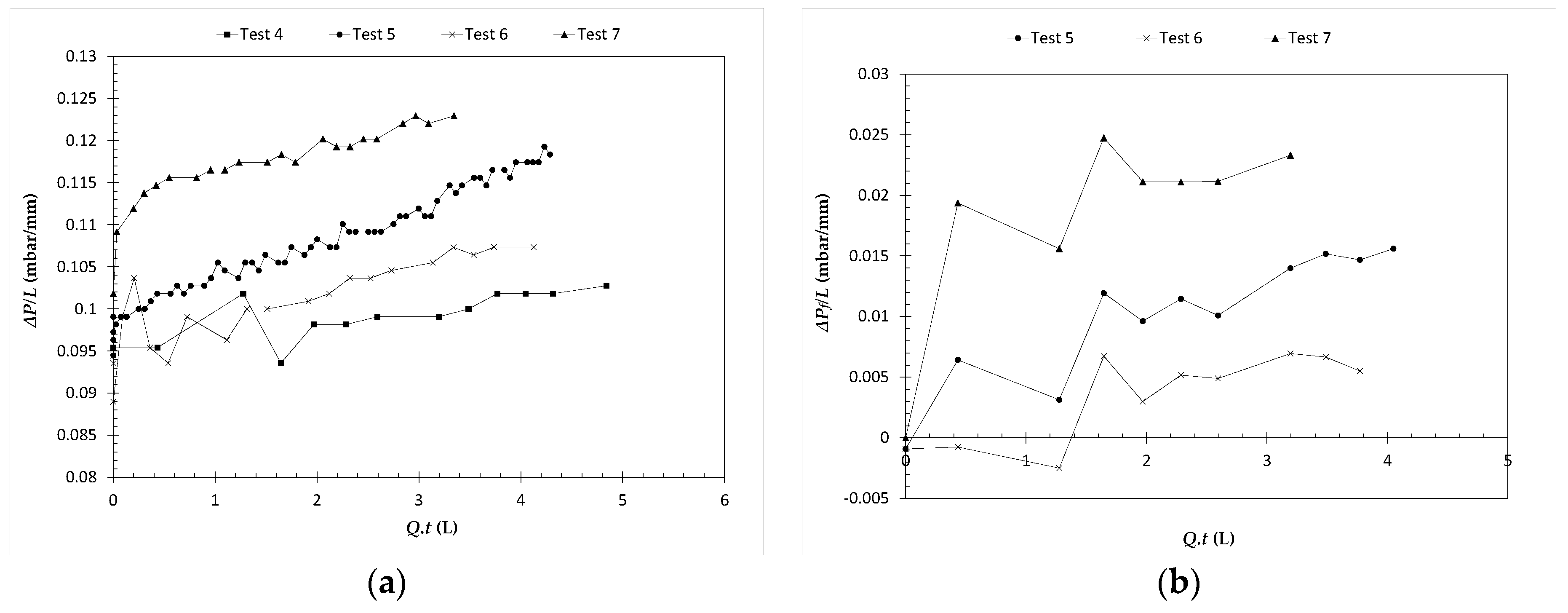
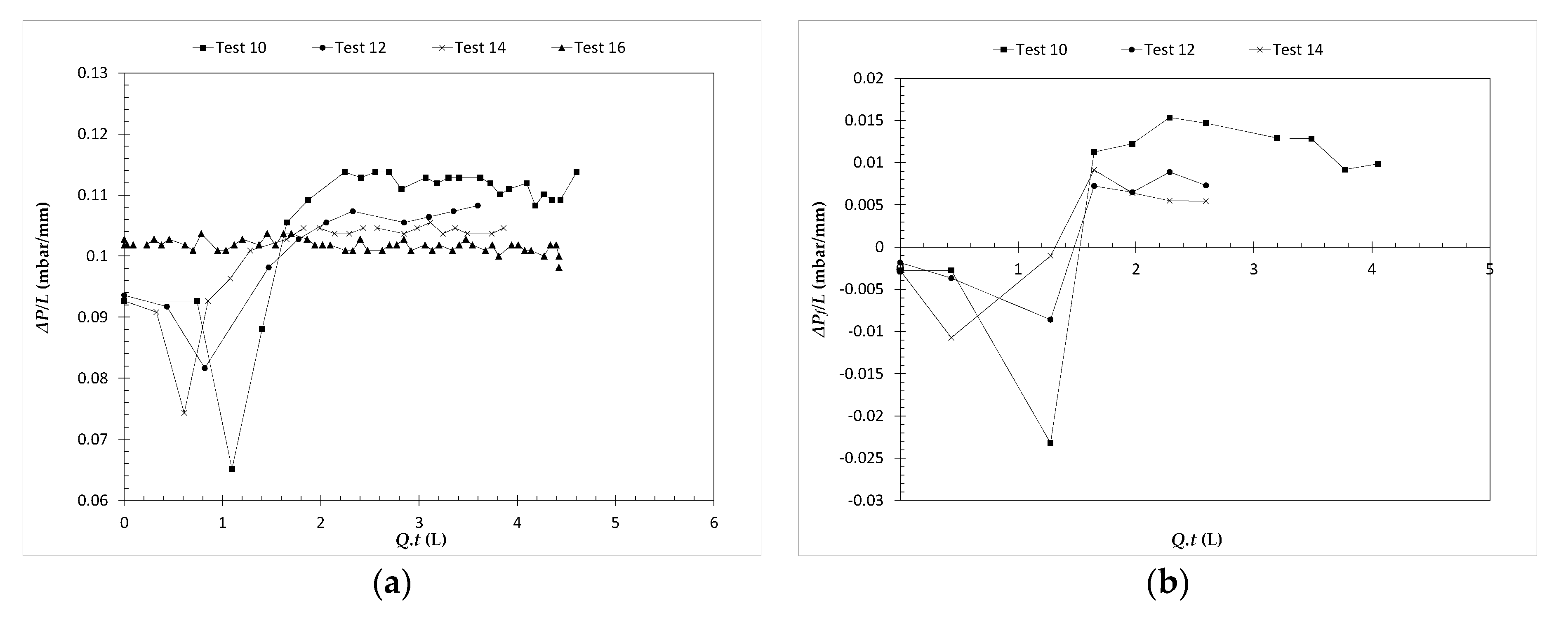
- While measured pressure gradients show an increasing trend for the whole period of the tests in the stable displacement tests, they initially increase in all unstable displacement cases and then become constant and continue due to the viscous fingering. The calculated frictional pressure gradients show increasing trends for stable displacement tests and increasing trends followed by decreasing trends for unstable displacement tests. A constant pressure gradient is observed in the whole period of the test with the bubble flow.
- In all cases consisting of stable and unstable displacements, proper tracking of the interface and fingers by the particles were observed. Tracing particles with different sizes and with intermediate densities on the interface always track the interface and move by it.
- Wetting of displaced fluid wall with the displacing fluid and changing the properties of front and back boundaries and the existence of side boundaries have no significant effect on the displacement pattern and efficiency.
Author Contributions
Funding
Institutional Review Board Statement
Informed Consent Statement
Data Availability Statement
Acknowledgments
Conflicts of Interest
References
- Nelson, E.B.; Guillot, D. Well Cementing; Schlumberger: Houston, TX, USA, 2006. [Google Scholar]
- Bishop, M.; Moran, L.; Stephens, M.; Reneau, W. A robust, field friendly, cement spacer system. In Proceedings of the AADE Fluids Conference and Exhibition, Houston, TX, USA, 8–9 April 2008. AADE-08-DF-HO-07. [Google Scholar]
- Lavrov, A.; Torsæter, M. Physics and Mechanics of Primary Well Cementing; Springer: Berlin/Heidelberg, Germany, 2016. [Google Scholar]
- Mitsuishi, N.; Aoyagi, Y. Non-newtonian fluid flow in an eccentric annulus. J. Chem. Eng. Jpn. 1973, 6, 402–408. [Google Scholar] [CrossRef]
- Jakobsen, J.; Sterri, N.; Saasen, A.; Aas, B.; Kjosnes, I.; Vigen, A. Displacements in eccentric annuli during primary cementing in deviated wells. In Proceedings of the SPE Production Operations Symposium, Oklahoma City, OK, USA, 7–9 April 1991. SPE Paper no. 21686. [Google Scholar]
- Nouri, J.M.; Umur, H.; Whitelaw, J.H. Flow of Newtonian and non-Newtonian fluids in concentric and eccentric annuli. J. Fluid Mech. 1993, 253, 617–641. [Google Scholar] [CrossRef]
- Nouri, J.M.; Whitelaw, J.H. Flow of Newtonian and non-Newtonian fluids in an eccentric annulus with rotation of the inner cylinder. Int. J. Heat Fluid Flow 1997, 18, 236–246. [Google Scholar] [CrossRef]
- Tehrani, A.; Ferguson, J.; Bittleston, S. Laminar displacement in annuli: A combined experimental and theoretical study. In Proceedings of the SPE Annual Technical Conference and Exhibition, Washington, DC, USA, 4–7 October 1992. SPE-24569-MS. [Google Scholar]
- Tehrani, A.; Bittleston, S.H.; Long, P.J.G. Flow instabilities during annular displacement of one non-Newtonian fluid by another. Exp. Fluids 1993, 14, 246–256. [Google Scholar] [CrossRef]
- Escudier, M.P.; Gouldson, I.W.; Jones, D.M. Flow of shear-thinning fluids in a concentric annulus. Exp. Fluids 1995, 18, 225–238. [Google Scholar] [CrossRef]
- Escudier, M.P.; Oliveira, P.J.; Pinho, F.T.; Smith, S. Fully developed laminar low of non-Newtonian liquids through annuli: Comparison of numerical calculations with experiments. Exp. Fluids 2002, 33, 101–111. [Google Scholar] [CrossRef]
- Malekmohammadi, S.; Carrasco-Teja, M.; Storey, S.; Frigaard, I.A.; Martinez, D.M. An experimental study of laminar displacement flows in narrow vertical eccentric annuli. J. Fluid Mech. 2010, 649, 371–398. [Google Scholar] [CrossRef]
- Kim, Y.; Han, S.; Woo, N. Flow of Newtonian and non-Newtonian fluids in a concentric annulus with a rotating inner cylinder. Korea Aust. Rheol. J. 2013, 25, 77–85. [Google Scholar] [CrossRef]
- Ytrehus, J.D.; Taghipour, A.; Werner, B.; Opedal, N.; Saasen, A. Experimental study of cuttings transport efficiency of water based drilling fluids. In Proceedings of the 33th International Conference on Ocean, Offshore and Arctic Engineering (OMAE2014), San Francisco, CA, USA, 8–13 June 2014; OMAE Paper no. 2014–23960. [Google Scholar]
- Ytrehus, J.D.; Taghipour, A.; Sayindla, S.; Lund, B.; Werner, B.; Saasen, A. full scale flow loop experiments of hole cleaning performances of drilling fluids. In Proceedings of the 34th International Conference on Ocean, Offshore and Arctic Engineering (OMAE2015), St. John’s, NL, Canada, 31 May–5 June 2015. OMAE Paper no. 2015–41901. [Google Scholar]
- Sayindla, S.; Lund, B.; Taghipour, A.; Werner, B.; Saasen, A.; Gyland, K.R.; Ibragimova, Z.; Ytrehus, J.D. Experimental investigation of cuttings transport with oil based drilling fluids. In Proceedings of the 35th International Conference on Ocean, Offshore and Arctic Engineering (OMAE2016), Busan, Korea, 19–24 June 2016. OMAE Paper no. 2016-54047. [Google Scholar]
- Bittleston, S.; Ferguson, J.; Frigaard, I.A. Mud removal and cement placement during primary cementing of an oil well-Laminar non-Newtonian displacements in an eccentric annular Hele-Shaw cell. J. Eng. Math. 2002, 43, 229–253. [Google Scholar] [CrossRef]
- Pelipenko, S.; Frigaard, I.A. On steady state displacements in primary cementing of an oil well. J. Eng. Math. 2004, 46, 1–26. [Google Scholar] [CrossRef]
- Pelipenko, S.; Frigaard, I.A. Two-dimensional computational simulation of eccentric annular cementing displacements. IMA J. Appl. Math. 2004, 69, 557–583. [Google Scholar] [CrossRef]
- Pelipenko, S.; Frigaard, I.A. Visco-plastic fluid displacements in near-vertical narrow eccentric annuli: Prediction of travelling-wave solutions and interfacial instability. J. Fluid Mech. 2004, 520, 343–377. [Google Scholar] [CrossRef]
- Iyoho, A.W.; Azar, J.J. An accurate slot-flow model for non-newtonian fluid flow through eccentric annuli. Soc. Pet. Eng. J. 1981, 21, 565–572. [Google Scholar] [CrossRef]
- Hele-Shaw, H.S. The flow of water. Nature 1898, 58, 33–36. [Google Scholar]
- Paterson, L. Radial fingering in a Hele Shaw cell. J. Fluid Mech. 1981, 113, 513–529. [Google Scholar] [CrossRef]
- Thome, H.; Rabaud, M.; Hakim, V.; Couder, Y. The Saffman–Taylor instability: From the linear to the circular geometry. Phys. Fluids Fluid Dyn. 1989, 1, 224–240. [Google Scholar] [CrossRef]
- Chen, J. Growth of radial viscous fingers in a Hele-Shaw cell. J. Fluid Mech. 1989, 201, 223–242. [Google Scholar] [CrossRef]
- Cardoso, S.S.S.; Woods, A.W. The formation of drops through viscous instability. J. Fluid Mech. 1995, 289, 351–378. [Google Scholar] [CrossRef]
- Miranda, J.; Widom, M. Radial fingering in a Hele-Shaw cell: A weakly nonlinear analysis. Phys. D 1998, 120, 315–328. [Google Scholar] [CrossRef]
- Praud, O.; Swinney, H.L. Fractal dimension and unscreened angles measured for radial viscous fingering. Phys. Rev. E 2005, 72, 011406. [Google Scholar] [CrossRef]
- Li, S.; Lowengrub, J.; Leo, P.H. A rescaling scheme with application to the long-time simulation of viscous fingering in a Hele–Shaw cell. J. Comput. Phys. 2007, 225, 554–567. [Google Scholar] [CrossRef]
- Fontana, J.; Dias, E.; Miranda, J. Controlling and minimizing fingering instabilities in non-Newtonian fluids. Phys. Rev. E 2014, 89, 013016. [Google Scholar] [CrossRef]
- Kondic, L.; Palffy-Muhoray, P.; Shelley, M.J. Models of non-Newtonian Hele-Shaw flow. Phys. Rev. E 1996, 54, 4536–4539. [Google Scholar] [CrossRef] [PubMed]
- Kondic, L.; Shelley, M.J.; Palffy-Muhoray, P. Non-Newtonian Hele-Shaw flow and the Saffman-Taylor instability. Phys. Rev. Lett. 1998, 80, 1433–1436. [Google Scholar] [CrossRef]
- Founargiotakis, K.; Kelessidis, V.C.; Maglione, R. Laminar, transitional and turbulent flow of herschel–bulkley fluids in concentric annulus. Can. J. Chem. Eng. 2008, 86, 676–683. [Google Scholar] [CrossRef]
- Maleki, A.; Frigaard, I.A. Tracking fluid interfaces in primary cementing of surface casing. Phys. Fluids 2018, 30, 093104. [Google Scholar] [CrossRef]
- Frigaard, I.A.; Maleki, A. Tracking fluid interface in carbon capture and storage cement placement application. In Proceedings of the 37th International Conference on Ocean, Offshore and Arctic Engineering (OMAE2018), Madrid, Spain, 17–22 June 2018. OMAE Paper no. 2018–77630. [Google Scholar]
- Taheri, A.; Ytrehus, J.D.; Taghipour, A.; Lund, B.; Lavrov, A.; Torsæter, M. Use of tracer particles for Tracking fluid interfaces in primary cementing. In Proceedings of the 38th International Conference on Ocean, Offshore and Arctic Engineering (OMAE2019), Glasgow, UK, 9–14 June 2019. OMAE Paper no. 2019–96400. [Google Scholar]
- Taheri, A.; Ytrehus, J.D.; Taghipour, A.; Lund, B.; Lavrov, A.; Torsæter, M. Experimental study of the use of particles for tracking the interfaces in primary cementing of concentric and eccentric wells. In Proceedings of the SINTEF Proceedings, Trondheim, Norway, 17–19 June 2019; pp. 91–99, ISSN 2387-4295. [Google Scholar]
- Qwabe, L.; Pare, B.; Jonnalagadda, S.B. Mechanism of oxidation of brilliant cresyl blue with acidic chlorite and hypochlorous acid. A kinetic approach. S. Afr. J. Chem. 2005, 58, 86–92. [Google Scholar]


| Parameters | Real Data | Down-Scaled Data |
|---|---|---|
| Length of the Cementing Section (l), m | 500 | 1 |
| Wellbore Size, inch | 16 1/2 | ---- |
| Casing Size, inch | 13 3/8 | ---- |
| Wellbore Radius (ro), m | 0.2096 | 0.05274 |
| Casing Radius (ri), m | 0.1699 | 0.04275 |
| Gap (h), m | 0.0397 | 0.01 |
| Pump Rate (Q), m3/s | 0.02 | 3 × 10⁻⁴ |
| Mean Flow Velocity (), m/s | 0.42 | 0.10 |
| Density of Displaced Fluid (ρ1), kg/m3 | 1440 | 1000 |
| Density of Displacing Fluid (ρ2), kg/m3 | 1800 | 1150 |
| Yield-Stress of Displaced Fluid (τy1), Pa | 4.79 | 0.16 |
| Yield-Stress of Displacing Fluid (τy2), Pa | 7.05 | 0.39 |
| Consistency Index of Displaced Fluid (κ1), Pasn | 0.02 | 1.29 |
| Consistency Index of Displacing Fluid (κ2), Pasn | 0.03 | 3.43 |
| Flow Behavior Index of Displaced Fluid (n1), dimensionless | 0.7 | 0.5 |
| Flow Behavior Index of Displacing Fluid (n2), dimensionless | 1 | 0.49 |
| Effective Shear Rate (γe), s−1 | 42.61 | 40.04 |
| Effective Viscosity of Displaced Fluid (µe1), Pas | 0.1189 | 0.2078 |
| Effective Viscosity of Displacing Fluid (µe2), Pas | 0.1955 | 0.5321 |
| Aspect ratio of circumferential and radial length scales (δ) | 0.033 | 0.033 |
| Aspect ratio of length and width scales (η) | 12598 | 100 |
| Reynolds Number (Re2) | 309.05 | 4.32 |
| Buoyancy Number (Bu) | 67.25 | 2.76 |
| Length of the Model (l), m | Width of the Model (d), m | Gap (h), m | Pump Rate (Q), m3/s | |
|---|---|---|---|---|
| 1 | 0.3 | 0.01 | 3 × 10⁻⁴ | 0.10 |
| Test | Fluid Type | pH | ρ (g/cc) | Carbopol (wt/wt %) | NaOH (wt/wt %) | Sucrose (wt/wt %) | NaCl (wt/wt %) | Glycerol (wt/wt %) | Blue Dye (wt/wt %) |
|---|---|---|---|---|---|---|---|---|---|
| 1 | Displaced | ----- | 1.00 | 0 | 0 | 0 | 0 | 0 | 0.000230 |
| Displacing | ----- | 1.15 | 0 | 0 | 35 | 0.0325 | 0 | 0.000000 | |
| 2 | Displaced | ----- | 1.00 | 0 | 0 | 0 | 0 | 0 | 0.000230 |
| Displacing | ----- | 1.15 | 0 | 0 | 35 | 0.0325 | 0 | 0.000000 | |
| 3 | Displaced | ----- | 1.00 | 0 | 0 | 0 | 0 | 0 | 0.000230 |
| Displacing | ----- | 1.15 | 0 | 0 | 35 | 0.0325 | 0 | 0.000000 | |
| 4 | Displaced | ----- | 1.00 | 0 | 0 | 0 | 0 | 0 | 0.000230 |
| Displacing | ----- | 1.15 | 0 | 0 | 35 | 0.0325 | 0 | 0.000000 | |
| 5 | Displaced | ----- | 1.00 | 0 | 0 | 0 | 0 | 0 | 0.000000 |
| Displacing | 7.40 | 1.15 | 0.1 | 0.035 | 35 | 0.0004 | 0 | 0.000000 | |
| 6 | Displaced | ----- | 1.00 | 0 | 0 | 0 | 0 | 0 | 0.000230 |
| Displacing | 7.00 | 1.16 | 0.1 | 0.030 | 0 | 0.0061 | 60 | 0.000000 | |
| 7 | Displaced | 7.80 | 1.00 | 0.08 | 0.032 | 0 | 0 | 0 | 0.000230 |
| Displacing | 7.40 | 1.15 | 0.1 | 0.035 | 35 | 0.0004 | 0 | 0.000000 | |
| 8 | Displaced | 7.80 | 1.00 | 0.08 | 0.032 | 0 | 0 | 0 | 0.000230 |
| Displacing | 7.40 | 1.15 | 0.1 | 0.035 | 35 | 0.0004 | 0 | 0.000000 | |
| 9 | Displaced | 7.50 | 1.00 | 0.1 | 0.039 | 0 | 0 | 0 | 0.000230 |
| Displacing | ----- | 1.15 | 0 | 0 | 35 | 0.0325 | 0 | 0.000000 | |
| 10 | Displaced | 7.50 | 1.00 | 0.1 | 0.039 | 0 | 0 | 0 | 0.000230 |
| Displacing | ----- | 1.15 | 0 | 0 | 35 | 0.0325 | 0 | 0.000000 | |
| 11 | Displaced | 8.00 | 1.00 | 0.08 | 0.039 | 0 | 0 | 0 | 0.000230 |
| Displacing | ------ | 1.15 | 0 | 0 | 35 | 0.0325 | 0 | 0.000000 | |
| 12 | Displaced | 8.00 | 1.00 | 0.08 | 0.039 | 0 | 0 | 0 | 0.000230 |
| Displacing | ------ | 1.15 | 0 | 0 | 35 | 0.0325 | 0 | 0.000000 | |
| 13 | Displaced | 8.00 | 1.00 | 0.08 | 0.039 | 0 | 0 | 0 | 0.000230 |
| Displacing | ------ | 1.15 | 0 | 0 | 35 | 0.0325 | 0 | 0.000000 | |
| 14 | Displaced | 8.00 | 1.00 | 0.08 | 0.039 | 0 | 0 | 0 | 0.000230 |
| Displacing | ------ | 1.15 | 0 | 0 | 35 | 0.0325 | 0 | 0.000000 | |
| 15 | Displaced | 7.10 | 1.00 | 0.1 | 0.032 | 0 | 0 | 0 | 0.000229 |
| Displacing | 6.50 | 1.15 | 0.1 | 0.032 | 35 | 0.0010 | 0 | 0.000000 | |
| 16 | Displaced | ------ | 1.14 | 0 | 0 | 35 | 0 | 0 | 0.000150 |
| Displacing | 7.00 | 1.00 | 0.1 | 0.032 | 0 | 0.0007 | 0 | 0.000000 |
| Test | ρ1 (g/cc) | ρ2 (g/cc) | τy1 (Pa) | τy2 (Pa) | κ1 (Pasn) | κ2 (Pasn) | n1 | n2 |
|---|---|---|---|---|---|---|---|---|
| 1 | 1.00 | 1.15 | 0.00 | 0.00 | 9.56 × 10⁻⁴ | 3.17 × 10⁻³ | 1.00 | 1.00 |
| 2 | 1.00 | 1.15 | 0.00 | 0.00 | 9.56 × 10⁻⁴ | 3.17 × 10⁻³ | 1.00 | 1.00 |
| 3 | 1.00 | 1.15 | 0.00 | 0.00 | 9.56 × 10⁻⁴ | 3.17 × 10⁻³ | 1.00 | 1.00 |
| 4 | 1.00 | 1.15 | 0.00 | 0.00 | 9.56 × 10⁻⁴ | 3.17 × 10⁻³ | 1.00 | 1.00 |
| 5 | 1.00 | 1.15 | 0.00 | 0.39 | 9.56 × 10⁻⁴ | 3.43 | 1.00 | 0.49 |
| 6 | 1.00 | 1.16 | 0.00 | 0.007 | 9.56 × 10⁻⁴ | 0.57 | 1.00 | 0.72 |
| 7 | 1.00 | 1.15 | 0.16 | 0.39 | 1.29 | 3.43 | 0.50 | 0.49 |
| 8 | 1.00 | 1.15 | 0.16 | 0.39 | 1.29 | 3.43 | 0.50 | 0.49 |
| 9 | 1.00 | 1.15 | 1.32 | 0.00 | 3.50 | 3.17 × 10⁻³ | 0.44 | 1.00 |
| 10 | 1.00 | 1.15 | 1.32 | 0.00 | 3.50 | 3.17 × 10⁻³ | 0.44 | 1.00 |
| 11 | 1.00 | 1.15 | 0.26 | 0.00 | 1.43 | 3.17 × 10⁻³ | 0.47 | 1.00 |
| 12 | 1.00 | 1.15 | 0.26 | 0.00 | 1.43 | 3.17 × 10⁻³ | 0.47 | 1.00 |
| 13 | 1.00 | 1.15 | 0.26 | 0.00 | 1.43 | 3.17 × 10⁻³ | 0.47 | 1.00 |
| 14 | 1.00 | 1.15 | 0.26 | 0.00 | 1.43 | 3.17 × 10⁻³ | 0.47 | 1.00 |
| 15 | 1.00 | 1.15 | 0.80 | 0.078 | 2.99 | 1.37 | 0.47 | 0.50 |
| 16 | 1.14 | 1.00 | 0.00 | 0.23 | 3.67 × 10⁻³ | 1.69 | 1.00 | 0.51 |
| No. | Particle Name | dp (µm) | ρp(g/cc) |
|---|---|---|---|
| 1 | Fluorescent Red Polyethylene Microspheres | 425–500 | 1.086 |
| 2 | Fluorescent Green Polyethylene Microspheres | 710–850 | 1.025 |
| 3 | Grey Polyethylene Microspheres | 850–1.0 | 1.05 |
| 4 | White Polystyrene Polymer Spheres | 2960 +/− 50 | 1.05 |
| Test | Displaced Fluid | Displacing Fluid | dp (µm) | Q (L/min) | (s−1) | Re2 | Bu |
|---|---|---|---|---|---|---|---|
| 1 | Water | Water + Sugar | 500 | 11.17 | 12.41 | 224.92 | 1520.55 |
| 2 | Water | Water + Sugar | 1000 | 12.48 | 13.87 | 251.30 | 1360.94 |
| 3 | Water | Water + Sugar | 500 | 16.01 | 17.79 | 322.38 | 1060.87 |
| 4 | Water | Water + Sugar | 1000 | 16.43 | 18.26 | 330.84 | 1033.75 |
| 5 | Water | Carbopol + Sugar | 1000 | 3.71 | 4.12 | 0.13 | 8.29 |
| 6 | Water | Carbopol + Glycerin | 500 | 11.81 | 13.12 | 2.74 | 17.67 |
| 7 | Carbopol | Carbopol + Sugar | 500 | 7.86 | 8.73 | 0.42 | 5.68 |
| 8 | Carbopol | Carbopol + Sugar | N/A | 6.46 | 7.18 | 0.31 | 6.23 |
| 9 | Carbopol | Water + Sugar | N/A | 12.02 | 13.36 | 242.04 | 1370.37 |
| 10 | Carbopol | Water + Sugar | N/A | 6.68 | 7.42 | 134.51 | 2465.84 |
| 11 | Carbopol | Water + Sugar | 500 | 15.46 | 17.18 | 311.31 | 1065.45 |
| 12 | Carbopol | Water + Sugar | 1000 | 15.17 | 16.86 | 305.47 | 1085.82 |
| 13 | Carbopol | Water + Sugar | 500 | 11.01 | 12.23 | 221.70 | 1496.08 |
| 14 | Carbopol | Water + Sugar | 1000 | 7.95 | 8.83 | 160.08 | 2071.93 |
| 15 | Carbopol | Carbopol + Sugar | N/A | 4.23 | 4.70 | 0.42 | 18.92 |
| 16 | Water + Sugar | Carbopol | N/A | 4.31 | 4.79 | 0.29 | −13.95 |
Publisher’s Note: MDPI stays neutral with regard to jurisdictional claims in published maps and institutional affiliations. |
© 2020 by the authors. Licensee MDPI, Basel, Switzerland. This article is an open access article distributed under the terms and conditions of the Creative Commons Attribution (CC BY) license (http://creativecommons.org/licenses/by/4.0/).
Share and Cite
Taheri, A.; Ytrehus, J.D.; Lund, B.; Torsæter, M. Use of Concentric Hele-Shaw Cell for the Study of Displacement Flow and Interface Tracking in Primary Cementing. Energies 2021, 14, 51. https://doi.org/10.3390/en14010051
Taheri A, Ytrehus JD, Lund B, Torsæter M. Use of Concentric Hele-Shaw Cell for the Study of Displacement Flow and Interface Tracking in Primary Cementing. Energies. 2021; 14(1):51. https://doi.org/10.3390/en14010051
Chicago/Turabian StyleTaheri, Amir, Jan David Ytrehus, Bjørnar Lund, and Malin Torsæter. 2021. "Use of Concentric Hele-Shaw Cell for the Study of Displacement Flow and Interface Tracking in Primary Cementing" Energies 14, no. 1: 51. https://doi.org/10.3390/en14010051
APA StyleTaheri, A., Ytrehus, J. D., Lund, B., & Torsæter, M. (2021). Use of Concentric Hele-Shaw Cell for the Study of Displacement Flow and Interface Tracking in Primary Cementing. Energies, 14(1), 51. https://doi.org/10.3390/en14010051