Abstract
In this paper, a nonlinear controller is proposed to manage the rotational speed of a full-variable Squirrel Cage Induction Generator wind turbine. This control scheme improves upon tractional vector controllers by removing the need for a rotor flux observer. Additionally, the proposed controller manages the performance through turbulent wind conditions by accounting for unmeasurable wind torque dynamics. This model-based approach utilizes a current-based control in place of traditional voltage-mode control and is validated using a Lyapunov-based stability analysis. The proposed scheme is compared to a linear vector controller through simulation results. These results demonstrate that the proposed controller is far more robust to wind turbulence than traditional control schemes.
1. Introduction
As concerns over the use of fossil fuels rise, renewable energy generation has received increased attention. In particular, wind energy conversion systems (WECS) have been growing in popularity for many years. The use of wind turbines to generate electricity has been increasing rapidly worldwide for multiple decades, with an estimated over 500 MW of installed capacity in 2018 [1].
Early iterations of wind turbine topologies, namely Type 1 configurations, employed simplified generator connections to the grid such that control of the systems was non-existent. Type 1 WECS typically involve the utilization of a SCIG with direct electrical connection to the grid with no ability for control. The descendants of these, Type 2 configurations, replaced the SCIG machine with a Wound Rotor Induction Generator, which through a rotor-connected resistor allows for slight speed control. Type 3 WECS typically incorporate Doubly-Fed Induction Generators alongside power converters to allow for improved speed control than that of a Type 2 or Type 1 [2]. However, these power converters only control the power that moves through the rotor of the machine. Recent iterations of wind turbine systems utilize the Type 4 configuration, which connects the generator to the grid through a pair of power electronic converters: a rectifier and an inverter, typically both controlled. The advantage these configurations have over their predecessors is that all power must go through these converters, meaning that they are 100% controllable [3]. Type 3 configurations only allow about 20% deviation from the synchronous speed of the grid they are connected to, which weakens their ability to be controlled. While these systems have traditionally employed the use of Permanent Magnet Synchronous Generators, recently designs are replacing them with Squirrel Cage Induction Generators (SCIG), which are much cheaper to produce than their counterparts [4]. A typical Type 4 SCIG system diagram is shown in Figure 1.
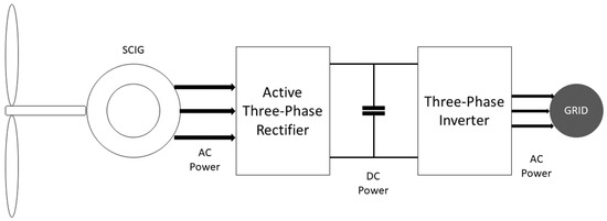
Figure 1.
Typical Type 4 SCIG configuration.
While Type 4 configurations utilizing SCIG are relatively new, the control of induction machines (IM) for motoring applications has been widely studied. Particularly, it is well known that two dynamics must be managed while controlling the speed of these machines: current and flux.
Early methods of speed management in IM, called scalar or volts-hertz control, involve providing three-phase voltages of a certain magnitude and frequency to the IM. The IM then rotates near the frequency of the voltages, and the magnitude manages the rotor flux [5,6].
As with most uncontrolled systems, open-loop scalar control suffers from large inaccuracies. From this, linear methods have been used to manage the synchronous speed provided to IM. Typically called slip control, these methods provide increased accuracy using proportional-integral (PI) control schemes [7]. In IM applications, the slip refers to the difference between the rotor and synchronous speeds, and by managing the slip, the synchronous speed is managed. These types of controllers can also be referred to as direct torque control (DTC), as controlling the slip ultimately serves to manage the electromagnetic torque of the IM.
However, even these slip control methods struggle due to their reliance on a single integrator to manage the speed. Hence, the electrical dynamics of IM influences a form of control known as vector control, in which a pair of cascaded PI controllers are used to manage the speed and flux separately. Vector control is performed in the rotating (dq) reference frame, so that the flux objective is met through the d-axis current and voltage and the speed objective is met through the q-axis current and voltage [8].
Notably, the ability to manage the flux in vector control is not trivial, as it is impractical to measure rotor flux in an IM in real time. Therefore, vector control heavily relies on the need for an accurate flux observer to maintain performance. Typically, these observers also provide a synchronous speed observation, which is needed to transform the dq voltages to the standard three-phase frame.
While vector control is popular even today, there are still issues with the linear control scheme it employs. While the cascading nature of vector control spreads the mathematical load across multiple controllers, PI-based control typically suffers from slow response times and difficulty with managing system nonlinearities.
To improve upon the aforementioned difficulties with both scalar and vector control, various improvements have been developed. A common improvement employs the use of fuzzy logic to better handle nonlinearities during operation. Fuzzy logic treats analog signals as continuously digital in nature, and categorically determines control inputs based on these “fuzzified” measurements. This strategy has been employed as a front-end scheme that determines the objectives for either scalar [9,10] or vector [11,12] PI controllers.
Another method used to improve vector control employs feedback linearization techniques. These schemes look to linearize nonlinear systems about a known operating point and control within that space [13]. While this greatly simplifies the mathematical model for control, it also makes the control less effective in any other operating point.
Another strategy for improving upon linear methods is the use of neural network control. This form of control attempts to estimate nonlinear functions that are unknown through repetitive learning algorithms [14].
Additionally, model-based methods have become more commonly used to manage parameter uncertainties and system nonlinearities. One nonlinear method that has been used is adaptive controls, which use model dynamics and measurable system states to estimate parameter uncertainties. Adaptive methods have been utilized for the purposes of both speed control [15,16,17] and flux observation [18,19].
Another nonlinear method that has been utilized for IM applications is sliding mode control (SMC). In SMC, the system is forced to slide along a cross-section of the system’s normal behavior using a model-based approach. These control schemes have been used similarly to both slip [20] and vector [21,22] objectives. While these controllers are typically good at managing parameter uncertainty, they also suffer from high computation time to function.
Yet another method for managing IM systems is model predictive control, in which parts of the mathematical model utilized for SMC or adaptive schemes are treated as unknown. These schemes predict changes in systems states based on measurable changes, which can compensate for system uncertainties [23,24].
As previously mentioned, Type 4 SCIG wind turbines have been studied little in comparison to other wind turbine systems. Some studies employ scalar control [25] or open-loop performance validation [26,27]. These studies ignored the control aspects of the system and instead focused on hardware validation. While these systems are not necessarily efficient, they successfully prove that SCIG are valid options for WECS.
A more recent application of SCIG as a wind turbine employs DTC and is validated using hardware in loop (HIL), which can accurately simulate real-time machinery [28]. This method tests the control scheme for various types of wind inputs, such as wind steps and turbulent wind profiles.
Most WECS systems thus far have employed some form of vector control to manage the rotational speed, as is typical in motoring applications. Due to the nature of wind speeds creating varying load torques, the selection of desired speeds and fluxes can be critical to operation. For this reason, some of these experiments utilize strategies that determine optimal desired flux values to minimize motor losses [29,30]. However, other experiments have shown that operation is possible without such an addition [31,32].
To improve upon the performance of traditional vector controllers, recent studies have used fuzzy logic to determine more optimal speed and flux trajectories [33,34,35]. These control schemes tend to focus on maximizing electrical power output rather than internal motor efficiency, which can potentially account for model or parameter inaccuracies.
Some more recent designs have used SMC to further improve the fidelity of the system control [36,37]. Wind turbines in particular present difficulty in ascertaining mechanical parameters, such as inertia and friction, due to the size and complexity of the mechanical subsystem. SMC is well-known for its ability to manage parameter uncertainty to improve performance.
Typically, all of the control methods mentioned thus far utilize voltage dynamics as the control input to the SCIG. However, there are numerous studies that exploit current dynamics instead using current-source converters (CSC). While the power electronic interface is relatively the same, working in a current-mode operation has some advantages, such as higher horsepower operation and reduced stator terminal stress [38,39].
In this paper, a model-based nonlinear controller is proposed to manage the rotational speed of a SCIG using a CSC. This controller is able to maintain high fidelity control through unknown wind torque characteristics. Turbulent wind speeds add high nonlinearity to speed control endeavors. The proposed controller also manages the potential for inaccurate mechanical parameters by utilizing adaptive measures to compensate for that uncertainty. It is commonplace in IM applications for mechanical inertia and friction to vary from the environment and wear. Additionally, the proposed scheme is able to manage the generator flux without the need for an observer, which presents a large advantage over vector control schemes.
The paper is organized as follows. Section 2 gives an overview of the mathematical system model. Section 3 provides the proposed controller framework with stability analysis. Section 4 provides test results using a simulation platform. Section 5 gives concluding remarks, and the last part includes references.
2. System Model
The rotational dynamics of a SCIG wind turbine can be modeled in the stationary () reference frame [37] as
where is the rotational velocity (in rad/s) of the wind turbine shaft, is the total turbine inertia, is the mechanical load torque, is the generator stator current, is the generator rotor flux, is a skew-symmetric matrix, and where is the number of generator pole pairs, is the generator mutual inductance, and is the generator rotor inductance. The definition of can be found as
where is the power of the wind captured at the turbine. This can be found through [37]
where is the density of the air, is the swept area of the turbine blades, is the wind velocity, and is the power coefficient of the turbine. This coefficient is analogous to the blade efficiency that has a maximum value equal to the Betz Limit, and is a function of the blade angle and the tip speed ratio (TSR) , which is defined as [37]
where is the radius of each turbine blade. The power coefficient, , is highly nonlinear and unmeasurable, but its behavior has been estimated [40,41]. Though there is variation in the exact expression used, the general mathematical form is largely agreed upon, as shown in Figure 2 [42].
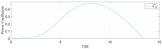
Figure 2.
Example of the power coefficient as a function of the TSR.
The electrical dynamics for a SCIG system can be modelled in the stationary reference frame as [37]
where is the generator stator voltage, , is the generator rotor resistance, is the generator stator inductance, and is the generator stator resistance.
3. Proposed Controller
The objective of this controller is to manage the rotational velocity, , of the wind turbine shaft such that it follows the desired speed trajectory, . This speed regulation is accomplished by managing the frame currents at the output of the SCIG. Ultimately, the goal of this system is to achieve maximum power output, which can be accomplished through the choice of speed trajectory.
Hence, the purpose of the proposed control scheme is to manage such that , which, based on the selection of , implies that , where is the maximum power able to be mechanically extracted from the wind.
This should be accomplished alongside the following assumptions.
Assumption 1.
The turbine torque
is an unknown time-varying quantity that is bounded by a known function , where is continuously differentiable. It is assumed that .
Assumption 2.
The generator flux
is assumed to be an unknown time-varying quantity.
Assumption 3.
The electrical parameters andare known a priori and are assumed to be constant with respect to time.
Assumption 4.
The mechanical turbine inertia
is assumed to be unknown and slowly time-varying such that .
Assumption 5.
The wind speed is assumed to be unknown. However, an upper bound for the wind speed,, is assumed to be known a priori and constant with respect to time.
Assumption 6.
The desired speed trajectory and flux magnitude and their derivatives,
, are assumed to be known and bounded (i.e., ).
Assumption 7.
The rotational velocity,
, of the turbine shaft is measurable.
To begin, an error signal is defined as
where is the desired speed trajectory. From this, a filtered error signal can be defined as
where is a positive constant. From the form of (8) it is clear that as , . Therefore, the goal of this controller is that remains bounded as .
As previously mentioned, a crucial piece to SCIG control is management of the generator flux . Therefore, a flux tracking error is also defined as
where the goal of the controller is for is bounded as . Additionally, the desired flux is defined as
where is a known desired flux magnitude and is the subsequently designed function for the synchronous angle of the SCIG.
The current command (i.e., the control signal to the SCIG) is implemented as
where are the subsequently designed equivalent currents in the rotating reference frame, as transformed about . By rearranging (10) and substituting dynamics from (9), the current can be rewritten as
3.1. Speed Error Dynamics
The control development begins by taking the time derivative of (7) and multiplying through by to obtain
which, after substituting the derivative of (6), can be rewritten as
Substituting (1) into (13) yields
Rearranging (8) and then substituting into (14) yields
where
is the desired torque of the SCIG. Based on the form of (16), the q-axis current can be defined as
To implement the above, the desired torque is defined as
where is a positive control gain, is a small constant, is a subsequently designed observer for the turbine inertia, and is defined as
where is the known upper bound of the wind speed and is the known upper bound of the mechanical friction.
Remark 1.
The term is a robust high-gain term designed to compensate for the unknown dynamics of . The function is chosen as an upper bound for the torque , which is inferred from (2). Since is an efficiency of the wind captured by the turbine blades, removing it from provides the power of the wind itself, which, alongside an upper bound for the wind speed, can be used as an upper bound on . The second term is added to compensate for potential friction dynamics in the generator.
After substituting the desired torque, the closed-loop mechanical dynamics become
3.2. Flux Error Dynamics
To obtain the d-axis current , the flux dynamics of the system are used. Taking the derivative of (8) yields
which can be further rewritten by substituting in (5) as
where
After substituting in dynamics from (8) and (9), (22) can be rewritten as
where
Substituting (10) and (17) into (24) yields
Here, the d-axis current and synchronous speed can be defined as
Substituting these back into (27) and thoroughly rearranging, the closed-loop flux dynamics become
A summary of the nonlinear controller is illustrated as a flow diagram in Figure 3.
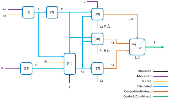
Figure 3.
Nonlinear control diagram.
3.3. Stability Analysis
Theorem 1.
The controlled currents implemented by (17), (28), and (29) ensure thatare Globally Uniformly Ultimately Bounded (GUUB).
Proof of Theorem 1.
The stability of the closed-loop system presented by the combination of (20) and (30) can be shown through a non-negative Lyapunov function , defined as
where is a positive control gain and
is the inertia observer error. Taking the derivative of (31) yields
Substituting (20) and (30) into (33) and simplifying yields
where
From this, the adaptive update law for the unknown turbine inertia can be defined as
Substituting this update law back into (34) yields
which from Assumption 1 can be upper bounded as
Upon inspection of the term, there become two possible cases. If , then (38) simplifies to
which is negative for all time. However, if , then (38) simplifies to
which requires further analysis.
Should (38) simplify to (40), the errors must be vectorized as
From this definition, can be redefined as
which, by using the Raleigh inequality, can be bounded as
where
From this, (40) can be rewritten as
where
Rearranging (46) yields the first order differential equation
where . Solving this differential equation yields
which from (43) can be rewritten as
Solving (50) for then yields
which will reduce to as .
The following signal chasing analysis will identify bounded signals in the closed-loop system. In this mathematical analysis, a term that belongs to is bounded.
From (51), it can be shown that . As stated in Assumption 6, and . Based on the definition of (7), it can be seen that . Then, from the form of (8), it is apparent that . From (19) it can be determined that . Then, it is apparent from (19) that . Then, the form of (17) indicated that . From (28) and (29), it can be shown that , respectively, and by extension . From the form of (9) and (10), it is apparent that , respectively. This utilization of standard signal chasing arguments shows that all signals in the closed-loop system remain bounded. Therefore, the system is Globally Uniformly Ultimately Bounded. □
Note that a closed-loop system that is GUUB infers boundedness for all time, with a magnitude of boundedness that is independent of time .
4. Simulation Results
The proposed controller has been tested and compared to a linear control scheme using PLECS simulation software. The parameters used for the SCIG WECS [28] is presented in Table 1.

Table 1.
System parameters for simulation platform of SCIG WECS.
4.1. Linear Controller Implementation
The linear controller used for comparison in this experiment is a cascaded Proportional-Integral (PI) controller [29], as shown in Figure 4. This is a voltage-mode vector control scheme, as is popularly used in IM and SCIG applications.
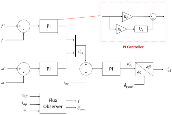
Figure 4.
Vector control architecture.
In the control scheme above, two separate control loops are used to manage the flux magnitude, , and the speed, , which output the desired dq current values, respectively. Note that all variables in Figure 3 with an asterisk are desired values. The vectorized current trajectory is then sent to a third control loop, which outputs a dq voltage.
The linear controller shown above has been appropriately tuned for optimal performance with respect to rotational speed control. In the case of these gains, the primary goal is minimization of response time. While it is theoretically possible for faster response time from linear controllers such as this, these gains reflect the fastest response whilst maintaining controller stability. As faster response time is achieved, the typical trade-off is larger overshoots, which when compounded with rapidly changing system conditions can cause controller instability. With this in mind, the control gains used are shown in Table 2.
Table 2.
Control gains for linear controller.
4.2. Experimental Methods
The proposed controller and the above vector controller have been tested for two experimental conditions. For the purposes of these experiments, the desired speed trajectory is calculated using a rearrangement of (4) as
where is a desired TSR. Note that the use of (52) does not override Assumption 5, as the controller itself doesn’t require knowledge of . The control objective values can be found in Table 3.
Table 3.
Desired values for SCIG control.
The first test utilizes a step in wind speed from 3 to 6 m/s. While an instantaneous step in wind speed does not occur realistically, this presents a worst-case scenario for the purposes of comparing each controller’s ability to respond to changes in operating point. This experiment illustrates the response time of each controller.
The second experiment involves a more realistic turbulent wind speed profile applied to each controller. As the wind speed changes, the controllers need to constantly adapt, which is a common occurrence in some locations. The goal of this test is to expose the average error of each controller over extended period of time.
4.3. Results
The parameters used in the nonlinear controller can be found in Table 4.
Table 4.
Control gains for nonlinear controller.
The results of the wind step test can be seen in Figure 5. It is evident from this that as the operating point shifts abruptly, the nonlinear controller is about 75 times faster than the vector controller. This illustrates that the proposed controller is better able to adapt to changing conditions. As previously mentioned, such a scenario as this is impossible is reality, but this highlights the ability of each controller to manage a sudden change in operation.

Figure 5.
Response of a vector controller (above) and nonlinear controller (below) to a step in wind speed.
Additionally, the illustrate the convergence of all error signals from Section 3, the error signals from the proposed controller are displayed in Figure 6, Figure 7 and Figure 8 during the same wind step experiment. Note that the flux error is not a realizable signal due to Assumption 2 but is available for viewing in a simulation environment here. It is evident from these figures that all errors in the closed-loop system for the nonlinear controller quickly converge to a near-zero value.
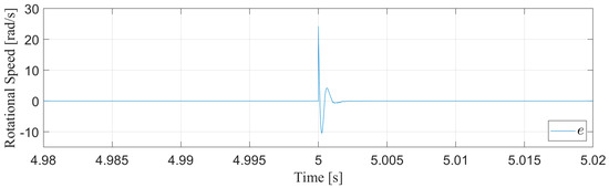
Figure 6.
Speed error during wind step.
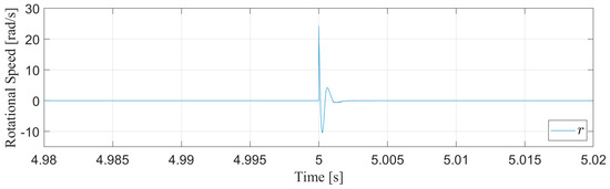
Figure 7.
Filtered speed error during wind step.
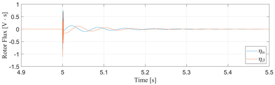
Figure 8.
Flux error during wind step.
It is also pertinent to show that the adaptive inertia term converges to a steady-state value. This can be shown for the wind step experiment in Figure 9. Note that the accuracy of this adaptive term is not a primary control objective.
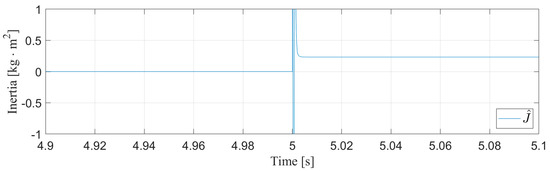
Figure 9.
Adaptive inertia observer during wind step.
The turbulent wind speed profile used for the second test is shown in Figure 10.
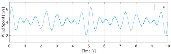
Figure 10.
Turbulent wind speed used for controller comparison.
As described by (52), this profile creates a desired speed trajectory as shown in Figure 11.
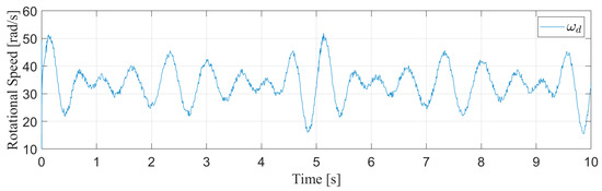
Figure 11.
Desired speed trajectory based on turbulent wind speed profile.
The results of applying this turbulence to each controller is displayed in Figure 12 in the form of the controller error . The RMS error of each controller indicates that the proposed scheme is about 250 times more precise than the vector control scheme. This illustrates that, in a realistic environment where turbulent wind speeds constantly ebb and flow, a SCIG control scheme must be able to manage the system to the desired trajectory through consistent disruption. These results clearly indicate that the proposed control scheme is superior to the performance of a typical linear controller.
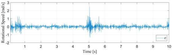
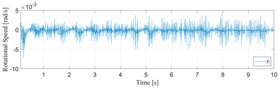
Figure 12.
Speed control errors of a vector controller (above) and nonlinear controller (below) in response to wind turbulence.
5. Conclusions
A nonlinear controller is proposed to increase the mechanical efficiency of a SCIG wind turbine system. The proposed scheme is compared to a traditional vector controller in simulation. Two comparative experiments are performed to evaluate the response time and average error of each controller. Results show that the proposed scheme is significantly faster and more precise than the traditional controller.
Beyond the performance results, this nonlinear controller also greatly simplifies the software implementation of a SCIG control. This method eliminates the need for voltage and current measurements, which are typically utilized in linear schemes. Additionally, the use of a linear flux observer (or any flux observation method) is not necessary with this approach. Instead, the only measurement necessary to implement the proposed controller is the rotational speed of the SCIG.
These results indicate the mathematical nature of this nonlinear controller is superior to typical linear control methods. However, this work does not illustrate a circuit-level implementation of this control system. As previously mentioned, this control assumes the utilization of a current–source converter to accurately apply the control signal (i.e., time-varying current) to the induction machine. Additional circuitry and mathematical analysis is needed to incorporate this power conversion method with the proposed nonlinear controller. Future work will investigate the integration of a current-source converter with this control scheme.
Author Contributions
Conceptualization, N.H. and M.L.M.; methodology, N.H. and M.L.M.; software, N.H. and B.B.; validation, N.H., B.B., and M.L.M.; formal analysis, N.H., B.B., and M.L.M.; investigation, N.H.; resources, M.L.M.; data curation, N.H. and B.B.; writing—original draft preparation, N.H.; writing—review and editing, B.B. and M.L.M.; visualization, N.H.; supervision, M.L.M.; project administration, M.L.M.; funding acquisition, M.L.M. All authors have read and agreed to the published version of the manuscript.
Funding
This research received no external funding.
Institutional Review Board Statement
Not applicable.
Informed Consent Statement
Not applicable.
Data Availability Statement
Data sharing not applicable.
Conflicts of Interest
The authors declare no conflict of interest.
References
- R.E.A. (IRENA). Wind Energy. 2018. Available online: irena.org/wind (accessed on 17 November 2019).
- Chen, Z.; Guerrero, J.M.; Blaabjerg, F. A review of the state of the art of power electronics for wind turbines. IEEE Trans. Power Electron. 2009, 24, 1859–1875. [Google Scholar] [CrossRef]
- Fateh, F.; White, W.N.; Gruenbacher, D. A Maximum power tracking technique for grid-connected DFIG-based wind turbines. IEEE J. Emerg. Sel. Top. Power Electron. 2015, 3, 957–966. [Google Scholar] [CrossRef]
- Goudarzi, N.; Zhu, W.D. A review on the development of wind turbine generators across the world. Int. J. Dyn. Control. 2013, 1, 192–202. [Google Scholar] [CrossRef]
- Srilad, S.; Tunyasrirut, S.; Suksri, T. Implementation of a scalar controlled induction motor drives. In Proceedings of the 2006 SICE-ICASE International Joint Conference, Institute of Electrical and Electronics Engineers (IEEE), Busan, Korea, 18–21 October 2006. [Google Scholar]
- Pena, J.M.; Diaz, E.V. Implementation of V/f scalar control for speed regulation of a three-phase induction motor. In Proceedings of the 2016 IEEE ANDESCON, Arequipa, Peru, 19–21 October 2016; pp. 1–4. [Google Scholar]
- Bechar, M.; Hazzab, A.; Habbab, M. Real-Time scalar control of induction motor using rt-lab software. In Proceedings of the 2017 5th International Conference on Electrical Engineering-Boumerdes (ICEE-B); Institute of Electrical and Electronics Engineers (IEEE): Boumerdes, Algeria, 2017; pp. 1–5. [Google Scholar]
- Jisha, L.; Thomas, A.A.P. A comparative study on scalar and vector control of Induction motor drives. In Proceedings of the 2013 International conference on Circuits, Controls and Communications (CCUBE), Bengaluru, India, 27–28 December 2013; pp. 1–5. [Google Scholar]
- Pati, S.; Patnaik, M.; Panda, A. Comparative performance analysis of fuzzy PI, PD and PID controllers used in a scalar controlled induction motor drive. In Proceedings of the 2014 International Conference on Circuits, Power and Computing Technologies [ICCPCT-2014], Nagercoil, India, 20–21 March 2014; pp. 910–915. [Google Scholar]
- Verma, P.; Saxena, R.; Chitra, A.; Sultana, R. Implementing fuzzy PI scalar control of induction motor. In Proceedings of the 2017 IEEE International Conference on Power, Control, Signals and Instrumentation Engineering (ICPCSI), Chennai, India, 21–22 September 2017; pp. 1674–1678. [Google Scholar]
- Kimiaghalam, B.; Rahmani, M.; Halleh, H. Speed & torque vector control of induction motors with Fuzzy Logic Controller. In Proceedings of the 2008 International Conference on Control, Automation and Systems, Seoul, Korea, 14–17 October 2008. [Google Scholar]
- Masoudi, S.; Feyzi, M.R.; Sharifian, M.B.B. Speed control in vector controlled induction motors. In Proceedings of the 2009 44th International Universities Power Engineering Conference (UPEC), Glasgow, UK, 1–4 September 2009. [Google Scholar]
- Chiasson, J. A new approach to dynamic feedback linearization control of an induction motor. IEEE Trans. Automat. Contr. 1998, 43, 391–397. [Google Scholar] [CrossRef]
- Wlas, M.; Krzeminski, Z.; Guzinski, J.; Abu-Rub, H.; Toliyat, H.A. Artificial-neural-network-based sensorless nonlinear control of induction motors. IEEE Trans. Energy Convers. 2005, 20, 520–528. [Google Scholar] [CrossRef]
- Talla, J.; Leu, V.Q.; Šmídl, V.; Peroutka, Z. Adaptive speed control of induction motor drive with inaccurate model. IEEE Trans. Ind. Electron. 2018, 65, 8532–8542. [Google Scholar] [CrossRef]
- Karagiannis, D.; Astolfi, A.; Ortega, R.; Hilairet, M. A nonlinear tracking controller for voltage-fed induction motors with uncertain load torque. IEEE Trans. Control. Syst. Technol. 2009, 17, 608–619. [Google Scholar] [CrossRef]
- Rashed, M.; MacConnell, P.; Stronach, A. Nonlinear adaptive state-feedback speed control of a voltage-fed induction motor with varying parameters. IEEE Trans. Ind. Appl. 2006, 42, 723–732. [Google Scholar] [CrossRef]
- Ohyama, K.; Asher, G.; Sumner, M. Comparative analysis of experimental performance and stability of sensorless induction motor drives. IEEE Trans. Ind. Electron. 2006, 53, 178–186. [Google Scholar] [CrossRef]
- Vonkomer, J.; Žalman, M. Induction motor sensorless vector control for very wide speed range of operation. In Proceedings of the 2011 12th International Carpathian Control Conference (ICCC), Velke Karlovice, Czech Republic, 25–28 May 2011; pp. 437–442. [Google Scholar]
- Rodić, M.; Jezernik, K. Speed-sensorless sliding-mode torque control of an induction motor. IEEE Trans. Ind. Electron. 2002, 49, 87–95. [Google Scholar] [CrossRef]
- Benchaib, A.; Edwards, C. Induction motor control using nonlinear sliding mode theory. In Proceedings of the 1999 European Control Conference (ECC), Karlsruhe, Germany, 31 August–3 September 1999. [Google Scholar]
- Horch, M.; Boumédiène, A.; Baghli, L. Backstepping approach for nonlinear super twisting sliding mode control of an induction motor. In Proceedings of the 2015 3rd International Conference on Control, Engineering & Information Technology (CEIT), Tlemcen, Algeria, 25–27 May 2015. [Google Scholar]
- Hedjar, R.; Toumi, R.; Boucher, P.; Dumur, D. A finite horizon cascaded nonlinear predictive control of induction motor. In Proceedings of the 2001 European Control Conference (ECC), Porto, Portugal, 4–7 September 2001. [Google Scholar]
- Diab, A.A.Z.; Vdovin, V.; Kotin, D.; Anosov, V.; Pankratov, V. Cascade model predictive vector control of induction motor drive. In Proceedings of the 2014 12th International Conference on Actual Problems of Electronics Instrument Engineering (APEIE), Novosibirsk, Russia, 2–4 October 2014. [Google Scholar]
- Nayanar, V.; Kumaresan, N.; Gounden, N.A. A Single-Sensor-Based MPPT Controller for Wind-Driven Induction Generators Supplying DC Microgrid. IEEE Trans. Power Electron. 2016, 31, 1161–1172. [Google Scholar] [CrossRef]
- Sasikumar, M.; Madhusudhanan, R.; ChenthurPandian, S. Modeling and analysis of cascaded H-bridge inverter for wind driven isolated squirrel cage induction generators. In Recent Advances in Space Technology Services and Climate Change 2010 (RSTS & CC-2010); IEEE: Chennai, India, 2010. [Google Scholar]
- Mesbahi, A.; Khafallah, M.; Saad, A.; Nouaiti, A. Emulator design for a small wind turbine driving a self excited induction generator. In Proceedings of the 2017 International Conference on Electrical and Information Technologies (ICEIT), Rabat, Morocco, 15–18 November 2017. [Google Scholar]
- Arafa, O.M.; Abdallah, M.E.; Aziz, G.A.A. Realisation and HIL testing of wind turbine emulator based on DTC squirrel cage inductor motor drive. Int. J. Ind. Electron. Drives 2018, 4, 155–168. [Google Scholar] [CrossRef]
- Pucci, M. Induction machines sensors-less wind generator with integrated intelligent maximum power point tracking and electric losses minimisation technique. IET Control. Theory Appl. 2015, 9, 1831–1838. [Google Scholar] [CrossRef]
- Abo-Khalil, A.G. Model-based optimal efficiency control of induction generators for wind power systems. In Proceedings of the 2011 IEEE International Conference on Industrial Technology, Auburn, AL, USA, 14–16 March 2011. [Google Scholar]
- Ferreira, J.C.; Machado, I.R.; Watanabe, E.H.; Rolim, L.G.B. Wind power system based on Squirrel Cage Induction Generator. In Proceedings of the XI Brazilian Power Electronics Conference, Praiamar, Brazil, 11–15 September 2011. [Google Scholar]
- Yan, Y.; Lin, F.; Wen, X.; Hu, G.; Zheng, T.Q. The Experimental system for variable-speed constant-frequency wind-power generation using induction machines. In Proceedings of the 2006 International Conference on Power System Technology, Chongqing, China, 22–26 October 2006. [Google Scholar]
- Kumar, C.; Sarma, A.; Prasad, P. Fuzzy logic based control of wind turbine driven squirrel cage induction generator connected to grid. In Proceedings of the 2006 International Conference on Power Electronic, Drives and Energy Systems, New Delhi, India, 12–15 December 2006. [Google Scholar]
- Mesemanolis, C.; Mademlis; Kioskeridis, I. High-efficiency control for a wind energy conversion system with induction generator. IEEE Trans. Energy Conver. 2012, 27, 958–967. [Google Scholar] [CrossRef]
- Brasil, T.; Crispino, L.; Suemitsu, W. Fuzzy MPPT control of grid-connected three-phase induction machine for wind power generation. In Proceedings of the 2015 IEEE 24th International Symposium on Industrial Electronics (ISIE), Buzios, Brazil, 3–5 June 2015. [Google Scholar]
- Hong, C.-M.; Lin, W.-M.; Cheng, F.-S. Application of Fuzzy Neural Network sliding mode controller for wind driven induction generator system. In Proceedings of the 2007 International Conference on Intelligent Systems Applications to Power Systems, Toki Messe, Niigata, Japan, 5–8 November 2007. [Google Scholar]
- Zribi, M.; Alrifai, M.; Rayan, M. Sliding mode control of a variable-speed wind energy conversion system using a squirrel cage induction generator. Energies 2017, 10, 604. [Google Scholar] [CrossRef]
- Salo, M.; Tuusa, H. A vector-controlled PWM current-source-inverter-fed induction motor drive with a new stator current control method. IEEE Trans. Ind. Electron. 2005, 52, 523–531. [Google Scholar] [CrossRef]
- Adamowicz, M.; Morawiec, M. Advances in CSI-fed induction motor drives. In Proceedings of the 2011 7th International Conference-Workshop Compatibility and Power Electronics (CPE), Tallinn, Estonia, 1–3 June 2011. [Google Scholar]
- Li, M.; Smedley, K. One-cycle control of PMSG for wind power generation. In Proceedings of the2009 IEEE Power Electronics and Machines in Wind Applications, Lincoln, NE, USA, 24–26 June 2009; pp. 1–6. [Google Scholar]
- Torki, W.; Grouz, F.; Sbita, L. A sliding mode model reference adaptive control of PMSG wind turbine. In Proceedings of the 2017 International Conference on Green Energy Conversion Systems (GECS), Hammamet, Tunisia, 23–25 March 2017. [Google Scholar]
- Abir, A.; Mehdi, D.; Lassaad, S. Pitch angle control of the variable speed wind turbine. In Proceedings of the 2016 17th International Conference on Sciences and Techniques of Automatic Control and Computer Engineering (STA), Sousse, Tunisia, 19–21 December 2016; pp. 582–587. [Google Scholar]
Publisher’s Note: MDPI stays neutral with regard to jurisdictional claims in published maps and institutional affiliations. |
© 2020 by the authors. Licensee MDPI, Basel, Switzerland. This article is an open access article distributed under the terms and conditions of the Creative Commons Attribution (CC BY) license (http://creativecommons.org/licenses/by/4.0/).