Abstract
Large rotating machinery, such as centrifugal gas compressors and pumps, have been widely applied and acted as crucial components in the oil and gas industries. Breakdowns or deteriorated performance of these rotating machines can bring significant economic loss to the companies. In order to conduct effective maintenance and avoid unplanned downtime, a system-wide health indicator is proposed in this paper. The health indicator not only uses a dynamic risk profile, but also considers financial loss and the fault probability based on condition monitoring data. This methodology is carried out by four steps: fault detection, probability of fault calculation, consequence of fault calculation and dynamic risk assessment. In our methodology, the fault probability is calculated by robust Mahalanobis distance, presenting as a system-wide feature from a sparse autoencoder fault detection model enabled early fault detection. The value of the health indicator is presented in financial loss, which assists in effective operational decision-making in a process system. To evaluate the performance of the proposed indicator, two case studies were carried out—one case tested on multivariate industrial data obtained from a pump, and another one tested on an industrial data set from a compressor. Results prove that the integrated health indicator can detect the faults at their incipient stages, indicate the degradation of the system with dynamically updated process risk at each sampling instant, and suggest an appropriate shutdown time before the system suffers severe damage. In addition, this methodology can be adapted to other machines’ health assessments, such as those of turbines and motors. The presented method of processing the industrial data set can benefit relevant readers.
1. Introduction
Maintenance aims to minimize or avoid the performance degradation and unplanned downtime caused by the inevitable degradation of machines over their service times and to keep them in good working condition. Lack of maintenance is one of the key reasons that has led to catastrophic consequences and significant economic losses in industry [1]. Therefore, an appropriate maintenance strategy is essential for companies to minimize their maintenance expenses and maximize profit [2].
Among the commonly used maintenance methods, the risk based inspection/maintenance (RBI/RBM), which aims to reduce the overall risks that may result in unexpected failures [3], is attracting more attention. Many companies report that RBI/RBM’s systematic approach to inspection and maintenance can not only improve safety but also reduce operating cost [4].
Although RBI/RBM can quantify the risk associated with a particular process activity, the quantitative risk assessment factor cannot be updated during the life of a process [5]. To overcome this, a dynamic risk assessment method has been developed, which can capture the time-dependent behavior of the system risk profile.
Bayes theorem is a popular algorithm used for dynamic risk assessment. Meel and Seider [6] applied Bayes theorem to dynamically update the estimates of accident probabilities, using near misses and incident data collected from similar systems. The hierarchical Bayesian model was applied to estimate the updated risk profile in [7,8]. In [9], Bayes theorem was combined with a bow-tie model to assess and update the risk profile in a sugar refinery.
Most existing dynamic risk assessment methods, as reviewed above, only use statistical data, i.e., count data of accidents or near misses (precursors) from similar systems, to update the estimated risk profile. A major drawback of these methods is that one must wait until accidents or near misses (precursors) occur before updating the estimation of the risk profile. Besides, statistical data are collected from similar systems, reflecting population characteristics but not fully accounting for the individual features of the target system.
Industry today seeks maintenance solutions based on real-time health monitoring of assets [10,11]. Instead of collecting data from similar systems, the condition monitoring data give information on the individual degradation process of the target system, providing an opportunity to update the risk factor before actual failure occurs. Therefore, introducing condition monitoring data in dynamic risk assessment could be a beneficial complement to the statistical data, towards a condition monitoring-based dynamic risk assessment [12].
There have been a few attempts in the direction of applying condition monitoring data into the dynamic risk assessment. Zadakbar et al. [13] proposed a multivariate risk-based fault detection and diagnosis method using Kalman filter to estimate the degradation states based on condition monitoring data and calculated the residual between the measured data and estimated data. Similar works were carried out by the same research group using different condition monitoring techniques, such as the control chart technique [14], principal component analysis (PCA) [15], and the particle filter [16]. Zeng and Zio [17] developed a dynamic risk assessment model by combining statistical failure data and condition monitoring data. However, most of the aforementioned methods do not involve consequence analysis models when calculating the risk profiles. In reference [13,14,15,16], the “consequence” in the risk model was replaced by a severity score for a fault designed for the applied fault detection method, i.e., control chart technique, PCA. In [17], the consequence analysis model was specially designed for a high-flow safety system in a tank.
Therefore, a literature review was carried out on the consequence analysis model, which is an important component of the dynamic risk assessment model. API RP 581 [18], published by American Petroleum Institute, is a risk-based maintenance standard applied for petrochemical equipment, such as tanks, compressors, and pumps. The consequences calculation method in [18] includes qualitive, semi-qualitive, and static quantitative models, lacking a fully quantitative consequence model that is applied on condition monitoring data. To quantify process losses, several researchers proposed different types of loss functions. Khan et al. [19] carried out a comprehensive review of these loss functions and discussed their application in detail. In the paper, an inverted beta loss function was applied for units requiring both the upper and lower boundaries of an operating variable; inverted normal loss function was used for units only requiring the upper boundary of an operating variable; and multivariate inverted loss function was employed for units requiring multivariate monitoring. More works on applying loss function in risk assessment can be found in [20,21,22].
However, irrespective of the good performance of the aforementioned works, some challenges remain in maintenance of machines in real industrial applications.
- On one hand, dynamic risk-based maintenance research [13,14,15,16,19,20,21,22] focuses on lowering the entire risk of the system, without putting much attention on the early detection of the fault. In the dynamic risk model, the fault/failure probability is heavily related to fault detection. Therefore, there is a requirement to improve the fault/failure probability calculation model with the application of advanced fault detection methods. Meanwhile, the loss function is suggested to be integrated into the risk model, as it can help estimate process economic risk and assist in effective operational decision-making.
- On the other hand, fault detection research [23,24,25,26] mainly focused on the development of an advanced model to detect an incipient fault, without considering the optimum time for maintenance. Most of the models [23,24,25] were tested on simulated or experimental data only, lacking the evaluation on real industrial data.
To address the aforementioned challenges, this paper proposes a system-wide health indicator using a dynamic risk profile, which takes into account both the financial loss and the fault probability based on condition monitoring data. In our methodology, the fault probability is calculated by robust Mahalanobis distance, measuring the difference between the condition monitoring data and the data under healthy conditions, and it is presented as a system-wide feature from a sparse autoencoder fault detection model, enabling early fault detection. The value of the health indicator is presented in financial cost, which assists in effective operational decision-making in a process system. The threshold setting is based on various literature reviews on anomaly detection [27,28,29] and an industrial standard (API 581) [18] by the American Petroleum Institute. The main benefits of the proposed method include early detection of faults, fault analysis, suggesting maintenance time, safety improvement, and minimum interruption of operation.
The rest of the paper is organized as follows. The proposed health indicator and the algorithms employed in this paper are explained in Section 2. Based on the proposed methodology, the performance of the health indicator was evaluated on multivariate industrial data obtained from a pump and a compressor; see Section 3 and Section 4 respectively. Finally, the conclusion and the main contributions are highlighted in Section 5.
2. Methodology
This section proposes a methodology to calculate a system health indicator, as presented in Figure 1. It consists of two phases: (1) an offline phase to develop the fault detection model and risk model, and (2) an online phase to detect make maintenance decisions. The detailed working mechanisms of these two phases are explained in the following two sub-sections.

Figure 1.
Flow chart of the proposed methodology to calculate integrated system health indicator (estimated maximum loss (), description presented in Section 2.1.3; is system wide feature in the offline phase; hM is system wide feature in the online phase; is the fault detection threshold in Mahalanobis distance; is the shutdown threshold in Mahalanobis distance; R1 is the fault detection threshold for the system health indicator (); is the shutdown threshold for the system health indicator.)
In the proposed methodology, the system health indicator is represented by the dynamic risk profile () of the system, which is calculated by the probability of fault () and consequence of fault (). The is derived from the offline training data under normal conditions and the is measured by financial loss using inversed normal distribution. The health indicator contains two stages of threshold. The threshold indicates a fault is detected in the system and suggests operators to take priority response (i.e., schedule a proper maintenance time). The threshold suggests a shutdown is required to ensure the safety running of the machine and avoid unplanned shutdown. The health indicator can be used for fault detection and for taking any supervisory decisions to activate appropriate safety systems in real time.
This work is a further development of our pervious work [1], where we developed a fault detection and isolation scheme based on sparse autoencoder (SAE), but did not take financial factors into consideration. This paper merged the system-wide feature, which is obtained by SAE and Mahalanobis distance (MD), and the financial consequences into a comprehensive system health indicator. The proposed health indicator can demonstrate the health condition of the system to the operator at real time, assist the operators on when an incipient fault is detected, how the system is degraded, what type of fault the machine suffers from, when the deadline is for maintenance.
2.1. Offline Phase—Model Development and Threshold Calculation
The offline phase builds three models, which are fault detection model, model, and model with application of history data under normal condition. Based on these models, the risk threshold () of the health indicator is calculated.
2.1.1. Fault Detection Model Training
2.1.1.1. Calculation of a System-Wide Feature
In this methodology, the fault detection model is built using the SAE. The MD calculates the statistical difference of the residual outputs between actual inputs and reconstructed outputs. Then, the statistical difference is used as a system-wide feature for fault detection and estimation.
The SAE is a special type of feedforward unsupervised neural networks. An advantage of the unsupervised neural network is that it can detect anomaly without data being labelled. While for conventional Artificial neural network (ANN) and other types of supervised ANN methods, the input and output of models should be identified by the operators. The SAE can be divided into an encoder and a decoder. The encoder extracts features from the input data, which is case-dependent and is defined in Section 3 and Section 4. The decoder reconstructs the autoencoder state back to the input data space. The structure of SAE can be found in Figure 2.

Figure 2.
Sparse autoencoder structure.
The SAE reconstructs the input vectors in the output layer using Equation (1).
where is the input vector, and is the reconstructed output. is the nonlinear function of SAE, which predicts output based on the input , using parameters and . The details of SAE mechanisms can be found in [30,31].
Then, the multivariate residuals between the input variables and the reconstructed outputs can be calculated by Equation (2).
To detect the existence of a fault, an integrated feature is developed based on the multivariate residuals. In our methodology, the Mahalanobis distance are applied. The MD is a unitless distance measurement, which considers the correlations among variables. It has been successfully applied for the anomaly detection in wind turbine data [27,28,29], and early fault detection in pumps [30].
In this paper, a robust MD [29,32] is calculated using Equation (3). It calculates statistical difference of the residual outputs between actual and estimated inputs and used as an integrated system-wide feature.
where is the Mahalanobis distance, is the robust measure of central tendency (the median) and is the inverse covariance matrix calculated from the sample population through the minimum covariance determinant estimator [29].
The MD considers all input variables of the process data. Any anomalies in the process data can cause changes in this integrated system-wide feature.
2.1.1.2. Estimation of Probability Density Function (PDF)
The distribution of system-wide feature () influences the following steps on threshold and calculation. Reference [27] used Weibull distribution on fault detection threshold estimation, while reference [29] applied kernel distribution. Reference [15] used Normal distribution on calculation, while reference [33] applied kernel distribution. In this paper, to make our model more accurate, we add a procedure to select the best-fitting probability distribution model for system wide feature among four well-known candidate distributions. The candidate distributions and their probability density functions (PDF) are summarized in Table 1.

Table 1.
The probability density function and their parameters.
In Table 1, the generalized extreme value distribution (GEVD) includes three types of extreme value distributions (see Figure 3), which are type I (), type II (), and type III ().

Figure 3.
Typical example PDF of type I, II, III distributions of GEVD.
The parameters of the distributions can be estimated using maximum likelihood estimation. The goodness-of-fit test should be performed to quantify how the selected distribution matches the original data. There are numerous statistical fitting tests, which are commonly used for evaluating the goodness of the distribution fitting. Some of the popular statistical fitting tests include Kolmogorov–Smirnov test (K–S) test, Anderson–Darling test, Cramer–von Mises test, chi-squared test, etc.
In this paper, K–S test [34] is applied to determine if a hypothesized distribution fits a data set. This test can be used for small and large sample sizes. The K–S test compared the sample’s empirical cumulative distribution function () () with the of a selected distribution . If deviates too much from , the null hypothesis is rejected. In this paper, the null hypothesis is that the selected distribution fits the sample data. The outputs of K–S test are and a value. is the decision whether to rejected the hypothesis or not. if the test rejects the null hypothesis at the 5% significance level, or 0 otherwise. The value is the probability of observing a test statistic as extreme as, or more extreme than, the observed value under the null hypothesis. Its range is [0, 1]. Small values of cast doubt on the validity of the null hypothesis.
2.1.1.3. Calculation of Thresholds
After getting the PDF function, the fault detection threshold can be obtained from the PDF function of for a given confidence level ( was applied [27]) by solving Equation (4):
In Equation (4), is the PDF function of the selected probability distribution of . The details of probability distribution selection can be found in Section 2.1.1.2.
If no corrective action was taken after a fault being detected, the online MD value would exceed the shutdown threshold . The value of this threshold based on the acceptable criteria of the specific process system. Alternatively, according to [20], when not enough information is available, the shutdown threshold of a measurement can be defined as 4 times larger than its maximum operating value.
where is a combination matrix, which covers any variables in the training data becomes 4 times larger than their normal operating values. The value of can also be given by the end users based on the acceptable criteria of the specific process system. is the reconstructed output. and are adopted directly from the training phase as calculated in Equation (3).
2.1.2. Build Probability of Fault () Model
The probability of fault () indicates the probability of a fault that happened on the piece of equipment. Hence, the of equipment should be calculated using measurements that can reflect the health status and degradation process of equipment. Usually, only one key variable is selected to calculate the probability, and this variable is expected to be the most sensitive one in the system [35]. In our methodology, the system wide feature () is selected for calculation.
A visual depiction of the proposed is presented in Figure 4. It ranges from 0 to 1. When no fault is detected in the system, ; when a fault or an anomaly is detected, ; if no maintenance actions are taken after a fault is detected, the would keep increasing to 1.
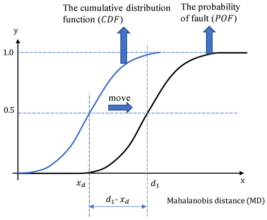
Figure 4.
The proposed probability of fault () model.
Note that, the means the system definitely has a fault, rather than a catastrophic failure. is a MD value for early fault detection. When the integrated system-wide feature () is greater than , there should be an early fault in the system. However, considering the fault detection method has false alarm rates, we adjusted the () to 0.5. If the system suffers a fault, it will cause further performance degrading, and the system-wide feature () will increase to 1.
In Figure 4, the blue curve is the cumulative distribution function () of a standard distribution, and it can be express as:
where is the probability density function depend on the selected distribution.
The offline model (black curve in Figure 4) is obtained by moving the to a new position, with the horizontal movement distance equals . The can be calculated by solving Equation (7).
where is the probability density function depending on the selected distribution for the training data. The details of probability distribution selection can be found in Section 2.1.1.2.
Therefore, the is expressed in Equation (8):
where is the fault detection threshold for the fault detection model that were calculated during training stage using Equation (4). is the Mahalanobis distance in Equation (3).
When reaches 1, a fault is occurred in the system, however, as it is still in its early stage, the financial consequence is low. In order to fully use the remaining life of the machine, we calculated a shutdown threshold , which is calculated using method that was proposed in reference [2] and an industrial standard API 581 [3].
2.1.3. Build Consequence of Fault () Model Using Loss Function
The consequence of fault () is to quantify the potential consequence of the fault scenario and the loss function is employed for the calculation of . In condition monitoring process, the process loss starts to increase if the high-contributing process variables exceed their normal operation thresholds, and the maximum process loss is reached after any of the identified variables breach the shutdown threshold [22]. The loss function used to quantify the process loss is the inverted normal loss function, which is the most widely used pattern for describing random variables [19]. The loss function is given by Equation (9) [19,22].
In Equation (9), represents the estimated maximum financial loss based on the worst conditions and it can be calculated as:
where is downtime production loss, is the material cost, is the labor cost, is the technical support cost, is the economic consequence of asset loss, is the economic consequence of human health loss, and can include environmental clean-up cost, indirect costs that represent secondary effects, etc.
In Equation (9), represents the Mahalanobis distance calculated by Equation (3), is the target value of variable when financial loss is zero [19]. Hence, in this case. is the shape parameter defining at which value of the process variable when the maximum loss is reached. The shape parameter is calculated using Equation (11) by the least squares method.
where is the financial loss based on the worst case conditions, is the value when MD reaches the shutdown threshold . The shutdown threshold is set to ensure the safety running of the machine, avoid unplanned shutdown and high financial loss. In our case, when the performance feature exceeds its shutdown threshold, the degradation of a machine can increase rapidly, or its performance becomes very difficult to predict. At this circumstance, a machine is in a very dangerous situation, but there still exist a bit of time for the faulty machine to reach its maximum financial loss. In this case, the financial loss is set to 50% [20] of when MD reaches the shutdown threshold , which means .
In our case, we assume that critical faults can be detected by condition monitoring and fault detection system. Therefore, when a fault not be detected, is given an initial value (), which is composed of inspection cost and production loss that are caused by shutdown inspection. When a fault is detected, the fault analysis scheme would analyze the cause of the fault and infer the fault type, hence, the value would be updated according to the possible fault type.
2.1.4. Calculate Health Indicator and Threshold
The system health indicator is determined by risk, which depends on two factors: the probability of occurrence of a fault leading to an unwanted event () and consequence of the event (). The system health indicator is given by:
The operation of complex industrial processes is often subjected to multiple constraints to prevent catastrophic failure. These constraints are set at fault detection threshold and shutdown threshold for critical process variables.
The fault detection threshold can be calculated at the offline phase using the initial value of :
where is the fault detection threshold of MD using Equation (4). is the Mahalanobis distance calculated by Equation (7). is the initial estimated maximum financial loss before a fault being detected. is the shape parameter of the loss function, calculated by Equation (11).
2.2. Online Phase—Fault Detection and Decision Making
To monitor the system health at real time, the online phase calculates a health indicator based on dynamic risk profile of the system. Two key parameters, and of the risk profile, are updated by applying condition monitoring data into the offline models. In the online phase, after a fault is detected, the fault analysis system will help operators to deduce the possible fault type. The and shutdown threshold () can be updated for a specific fault. The comparison of the real time value of the health indicator () with fault detection threshold () and shutdown threshold (), provides guidance for operators on maintenance decision making.
2.2.1. Calculate Probability of Fault ()
In the online fault detection phase, the monitoring data are fed to the SAE model trained offline. The MD at online monitoring stage is calculated as
where and are adopted directly from the training phase as calculated in Equation (3). is the residual between the actual measurement values and the reconstructed output obtained using the trained SAE fault detection model.
The at online monitoring stage can be calculated as:
where is the MD at online monitoring stage. is the fault detection threshold presented in MD, and the value of is given in Equation (4). is the Mahalanobis distance calculated by Equation (7).
2.2.2. Calculate Consequence of Fault ()
The consequence of an unwanted event can be largely influenced the fault type of the machine. In this section, the fault type is achieved by fault analysis using a two-dimensional statistic contribution map, which stacks multiple observations (time point) into one image to clearly illustrate the contribution of the variables over the entire faulty data times series.
The statistic (also called squared prediction error, SPE) is widely used in process control for condition monitoring data [36,37,38]. The traditional statistic contribution plot can be calculated by Equation (19) [39]:
The conventional contribution plot is a one-dimensional plot, which only examines the contributions at one time point (one observation), and multiple contribution plots are needed to illustrate multiple observations in time series data. In contrast, a two-dimensional contribution map [40] stacks multiple observations into one image to clearly illustrate the contribution of the variables over the entire faulty data times series, which enables the fast identification of faulty variables within large heterogeneous data sets. Therefore, in our methodology, a two-dimensional statistic contribution map is applied for data analysis.
The fault analysis result updates the value of estimated maximum financial loss via Equation (10).
Therefore, the consequence in the online phase is calculated as:
where is the estimated maximum financial loss. When no fault is detected, the remains its initial value , which is described in Section 2.1.3. When a fault is detected, the should be updated according to the inferred fault type.
2.2.3. Calculate System Health Indicator and Shutdown Threshold
Combining Equations (16) and (18), a general system-wide health indicator using dynamic risk profile at online monitoring stage is expressed as:
The shutdown threshold is calculated as
where is the shutdown threshold of MD in Equation (5). is the estimated maximum financial loss for a specific fault type. Alternatively, the shutdown threshold can be decided by operators according to the maximum risk that a company can take.
To ensure the system risk within the acceptable range, two constraints ( and ) are set at fault detection threshold and shutdown threshold. These constraints can be decided by operators or calculated using Equations (13) and (20). The health indicator can be used for fault detection and for taking any supervisory decisions to activate appropriate safety systems in real time. If , it indicates that the health indicator at the monitoring stage is under the fault detection threshold. Therefore, the system is healthy during this status. If , it means that health indicator exceeds the fault detection threshold (). If the health indicator continuously exceeds , suggests operators to take priority response, for example, order inspection equipment, buy maintenance materials, and schedule a proper maintenance time. The fault analysis scheme calculates the contribution of each measurements, infers the possible fault types, and suggests the maintenance planning. If , it indicates the system is under a dangerous condition, and thereafter, the automatic safety system (i.e., emergency shutdown system) would be activated to avoid unplanned shutdown.
The value is a fault detection threshold in Mahalanobis distance, without considering any financial factors. It is obtained at confidence level of the training data, which means that we assume 99% of the training data is healthy and 1% is anomalies [30].
is the fault detection threshold, which is calculated based on and taken financial factors into consideration.
The value is a shutdown threshold in Mahalanobis distance. can be adjusted by operators according to system requirement. is the shutdown threshold, which is calculated based and taken financial factors into consideration to help operators make maintenance decision.
3. Case One: Health Indicator Applied on a Pump Data Set
To demonstrate the effectiveness of the proposed methodology in Section 2, a case study was carried out based on a group of multivariate data collected from a pump system in an oil and petrochemical factory. In this case, a comprehensive health indicator was developed for the pump, which can achieve the early detection of a fault, deduce the possible fault types according to a two-dimensional Q statistic contribution map, and provide a suggested maintenance time to make full use of the remaining life of the pump whilst avoiding unplanned shutdowns.
3.1. Data Description
Centrifugal high-pressure injection pumps some one of the most common pump types used in the oil and petrochemical industry for oil transportation, lift, and injection. Such pumps are likely to be subjected to performance degradation, because they are typically operated under high rotating speed, high pressure, and high loading conditions. The data used in this case study were obtained from a multivariate condition monitoring system mounted on a high-pressure injection pump in an oil and petrochemical plant in Europe, with sampling rate of one sample per hour. The measured variables are listed in Table 2. The training data were pre-processed to filter out the missing and erroneous data before feeding into the fault detection and fault analysis model.
Table 2.
Measurement variables in the pump monitoring system.
3.2. Offline Phase—Model Development and Threshold Calculation
In this study, the fault detection model was trained on the data acquired in a quarter of the year period from 10 March 2013 to 21 June 2013, where no abnormal events were recorded in the pump. The model was then used to assess the health condition after 22 June 2013. The offline model generation and thresholds calculations are shown in Section 3.2.1, and the online model testing results are presented in Section 3.2.2.
3.2.1. Fault Detection Model Training
The SAE fault detection model was trained on the pump data from 10 March 2013 to 21 June 2013. In SAE model, the number of nodes in the hidden layer was set as 11. This value was set according to our previous work presented in [30], where nodes numbered from 10 to 18 could all get good results on incipient fault detection for several cases, with a high fault detection rate of around 99%, while producing few false alarms. The MD between the reconstructed and original training data was calculated as using Equation (3), and its histogram can be seen in Figure 5a. The four candidate distributions were generalized extreme value, lognormal, normal, and kernel distributions. According to K–S test, is the null hypothesis that the selected distribution fits the sample data. if the test rejects the null hypothesis at the 5% significance level, and means the test accepts the null hypothesis. Therefore, the best fitted distribution should have the highest value and . The results of fitting distribution of MD between the reconstructed and true training data can be seen in Figure 5b,c. The results of the K–S test are listed in Table 3.
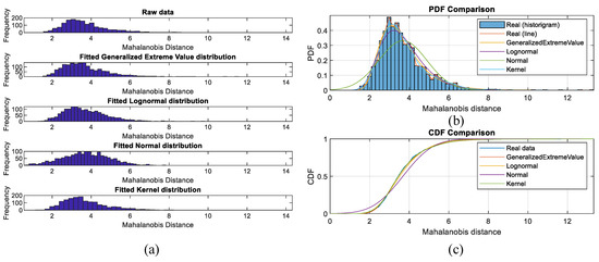
Figure 5.
Results of distribution fitting using training data: (a) histogram; (b) probability density functions; (c) cumulative distribution function.
Table 3.
Results of K–S test for case one.
According to Section 2.1.1.2, the output of the K–S test indicates the test distribution fits the input data. The value is the probability of observing a test statistic as extreme as, or more extreme than, the observed value under the condition of . The higher the value, the better the fitting. Therefore, from the table, the kernel distribution was selected. By maximum likelihood estimation, the parameters of the fitted kernel distribution were bandwidth = 0.223292 and kernel type of normal kernel.
After the distribution was selected, the fault detection threshold () was calculated based on Equation (4) with confidence level [27]. In other words, 99% of the training data are viewed as healthy data, and 1% are anomaly data. In this case, the calculated is equal to 7.41.
The offline fault detection model training result for an industrial pump from 10 March 2013 to 21 June 2013 by SAE is presented in Figure 6. In the figure, the magenta line is the fault detection threshold , the blue points under the threshold are healthy data, and the red points above the threshold are treated as anomaly data.
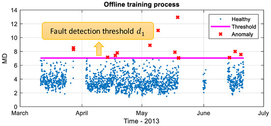
Figure 6.
Offline fault detection model training for an industrial pump from 10 March 2013 to 21 June 2013 by the sparse autoencoder (SAE; blue points: healthy data; red points: anomalies; magenta line: reference MD thresholds).
Then, the shutdown threshold was calculated using Equation (5). In the equation, the combination matrix covering each variable in the training data becomes four times larger than its normal value [20,41]. In this case, is equal to 144.24.
3.2.2. POF Model
The risk calculation has two parts: and calculation. The model was developed in the offline phase, with the system wide feature (the Mahalanobis distance ) on the x-axis, against the values on the y-axis.
In Equation (7), is the probability density function of kernel distribution, with parameters calculated in Section 3.2.1. Therefore, in this case, , and the offline model is presented in Figure 7. As can be seen, the was 0.5 when MD value equaled the fault detection threshold . In the offline model, when MD value was lower than , the value was lower than 0.5. When MD value was higher than , the was higher than 0.5 and could increase to 1. The value of the shutdown threshold was 1 when was equal to .
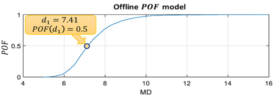
Figure 7.
Offline model for case 1.
3.2.3. COF Model Using Loss Function
The is assessed by loss function using Equations (9) and (10). By solving Equation (11) using the least squares method, with financial loss [20] and shutdown threshold calculated in Section 3.2.1, the shape parameter can be obtained as . Therefore, the default model can be written as: . In the offline phase, the used its initial value , which is composed of inspection cost and production loss that are caused by shutdown inspection. The value of would be updated in the online phase when a fault was detected.
3.2.4. Calculate Default Health Indicator Thresholds
The health indicator thresholds include a fault detection threshold () and a shutdown threshold (). Using the parameters calculated in Section 3.2.1 to Section 3.2.3, the fault detection threshold () equals 3587.3 ($), and shutdown threshold () will be calculated in the online stage after a fault is detected and the fault type is diagnosed.
3.3. Online Phase—Fault Detection and Decision Making
3.3.1. Calculating
The online phase was to use the trained SAE model to assess the health condition of the monitored pump using data recorded after 22 June 2013. The fault detection results for the pump from 22 June 2013 to 6 July 2013 can be seen in Figure 8. The MD value () for the online phase exceeds threshold after 3 July, which indicates a fault in the machine.
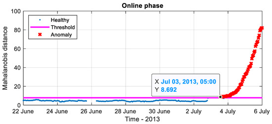
Figure 8.
Online testing results for an industrial pump from 22 June 2013 to 6 July 2013 by SAE model. (Blue points: healthy data; red points: anomalies; magenta line: reference MD thresholds).
Then, the values of the monitoring data were calculated using MD obtained in the online monitoring stage. The values of the pump system obtained by SAE based fault detection model are shown in Figure 9. As designed in Section 2.1.2 and Section 3.2.2, the fault detection threshold using was 0.5. The system would be in healthy condition with a value below 0.5. A fault condition was indicated once the value exceeded 0.5. The value showed that a fault occurred at 5:00 3 July 2013, which was consistent with that obtained using the MD value in Figure 8.
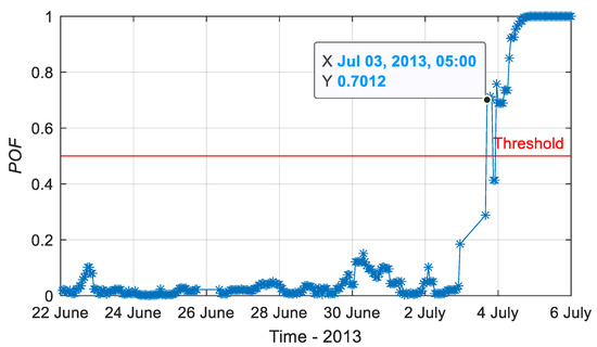
Figure 9.
of the pump system obtained by SAE in the online phase (red line: fault detection threshold )
3.3.2. Calculating
After a fault is detected, the fault analysis module will deduce the possible fault type, and therefore, update the value of the fault. In this paper, a two-dimensional Q statistic contribution map was calculated. As shown in Figure 10, an incipient fault was detected on 3rd July. Gradually, four bearings’ temperatures and discharge pressures started to show faults. The fault analysis worked in real time, and when a fault type is inferred, the financial factors will be updated accordingly. The results give maintenance staff a clear indication of bearing-related faults, e.g., bearing faults, misalignment, and rotor unbalance.
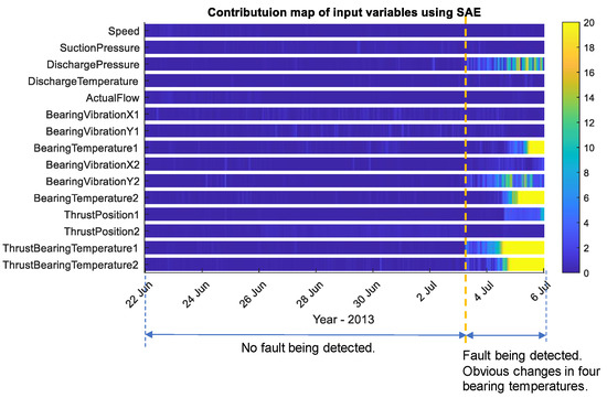
Figure 10.
Contribution map by the SAE model from 22 June 2013 to 6 July 2013.
After the fault type was inferred, the financial factors in estimated maximum financial loss () were updated by bearing-related faults, and the financial factors and their values are listed in Table 4. The at online phase can be found in Figure 11.
Table 4.
Financial factors and their values updated by bearing-related fault in the pump.

Figure 11.
Consequence of a fault occurring in the pump system updated by bearing-related fault.
3.3.3. Calculating the System Health Indicator
The system health indicator is a dynamic risk profile of the pump. It was obtained by combining the with the in the online phase. The system health indicator presented by risk profile of the pump is shown in Figure 12.
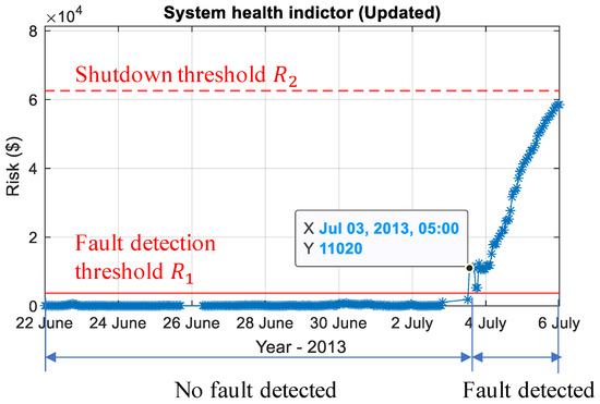
Figure 12.
System health indicator presented by risk profile of the pump.
In Figure 12, the first threshold was used for fault detection, which means that if the value exceeds the threshold, it is considered as a fault. This threshold also suggests to operators a priority for the response (i.e., schedule a proper maintenance time) to the detected fault. In this case, the health indicator gave warnings at 5:00, 3 July 2013. The start point of the fault was marked at the point that the health indicator continuously exceeded the . Comparing to the measured variables from the pump’s condition monitoring system in Figure 13, the health indicator successfully detected the fault at its incipient stage.
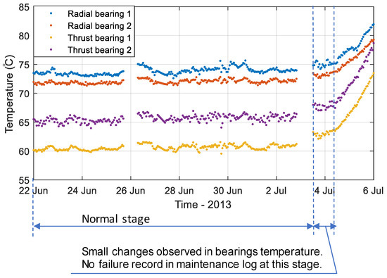
Figure 13.
The measured bearing temperature obtained from the pump’s condition monitoring system.
The second threshold in Figure 12 was used for system protection. was calculated in the online stage using Equation (20) after a fault being detected and fault type deduced. If no corrective action is taken or the corrective action fails to bring down the risk, the risk factor would exceed the second threshold. Then, the emergency shutdown system would be activated to avoid unplanned shutdown.
As the health indicator is updated with condition monitoring data, it can reflect the system’s health status at real time. It considers the probability of fault and financial loss, showing the system’s risk in dollars. All these features help maintenance decision making. The company shut down the pump when the risk was quite close to . The developed health indicator indicated that the maintenance action should be taken no later than 6 July to avoid the unplanned shutdown.
4. Case Two: Health Indicator Applied on a Compressor Data Set
In order to further assess the ability of the proposed methodology for effective incipient fault detection and maintenance work, the model was tested using data captured from an operational industrial compressor.
4.1. Data Description
The monitored variables for the compressor are listed in Table 5. The SAE model was trained on the data for a four month period from 22 April 2014 to 22 August 2014, where no faults were recorded in the compressor. The models were then used to assess the health condition from 23 August 2014 to 23 October 2014.
Table 5.
Monitoring variables for a compressor system.
4.2. Offline Phase—Model Generation and Threshold Calculation
The parameters of SAE model were set to be the same as in case one, with 11 nodes in the hidden layer. The MD between the reconstructed and the measured data is expressed as in Equation (3). The results of the K–S test are listed in Table 6. As can be seen, the kernel distribution fits best with this data set. The maximum likelihood estimation was then applied to estimate the parameters for the selected distribution. The fitted kernel distribution was normal kernel and the bandwidth was 0.186253.
Table 6.
Results of K–S test for case two.
After the distribution was selected, the fault detection thresholds () for the SAE model were calculated based on the training data using Equation (4) with confidence level [27]. The MD fault detection thresholds and were equal to 9.5590 and 28.6584, respectively.
The offline fault detection model trained for an industrial compressor from 22 April to 22 August 2014 by SAE is presented in Figure 14. In the figure, the magenta line is the fault detection threshold , the blue points under the threshold are healthy data (99% of the training data), and the red points above the threshold are treated as anomaly data (1% of the training data).
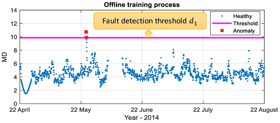
Figure 14.
Offline fault detection model trained for an industrial compressor from 22 April to 22 August 2014 by SAE. (Blue points: healthy data; red points: anomalies; magenta line: reference MD thresholds).
In the offline phase, the model was developed, with the system wide feature (the Mahalanobis distance ) on the x-axis, against the values on the y-axis. By applying the selected kernel distribution into Equation (7), can be calculated as .
The offline model was presented in Figure 15. As can be seen, the was 0.5 when MD value equaled the fault detection threshold . When MD value was lower than , the value was lower than 0.5. When MD value was higher than , the was higher than 0.5 and could increase to 1. This result was in accordance with the model designed in Section 2.1.2.

Figure 15.
Offline model for case 2.
The is calculated using Equations (9) and (10). By solving Equation (11) using least squares method, with financial loss [20], the shape parameter can be obtained. In this case, . Therefore, the default model can be written as: .
According to the aforementioned parameters, the fault detection threshold () of 9768.4 ($) was obtained. The shutdown threshold () was calculated in the online phase after a fault was detected and the fault type inferred.
4.3. Online Phase—Fault Detection and Decision Making
Figure 16 shows the health condition of the industrial compressor from 23 August 2014 to 23 October 2014. An incipient fault was detected during 22 September to 2 October, as the MD value continuously exceed the fault detection threshold. After 2 October, the health status of the compressor became worse as the MD value kept increasing.
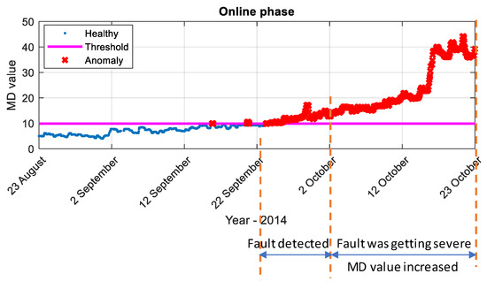
Figure 16.
Online testing results for an industrial compressor from 23 August to 23 October 2014 by SAE model. (Blue points: healthy data; red points: anomalies; magenta line: reference MD thresholds).
The risk calculation has two parts: and calculation. The of the industrial compressor for the online phase is shown in Figure 17. The fault detection threshold was 0.5. The fault detected time using value was 22 September 2014, which was consistent with that using MD value in Figure 16.
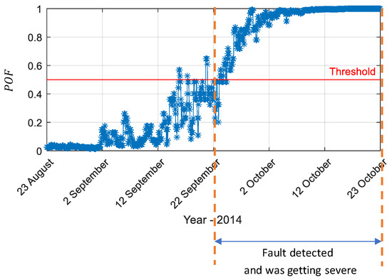
Figure 17.
of the compressor obtained by SAE in the online phase (red line: fault detection threshold )
The two-dimensional Q statistic contribution map in Figure 18 shows the contribution of each input variable to the detected anomaly. The figure clearly shows that stage 3 DE bearings’ measurements mainly contributed to the increase of the MD value.
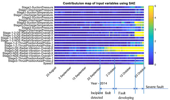
Figure 18.
Q statistic contribution map by SAE model from 23 August to 23 October 2014.
After the fault type was inferred, the financial factors in estimated maximum financial loss () were updated by bearing-related faults. The financial factors and their values for maintaining this compressor are listed in Table 7. The at online phase can be found in Figure 19.
Table 7.
Financial factors and their values updated by bearing-related fault in the compressor.
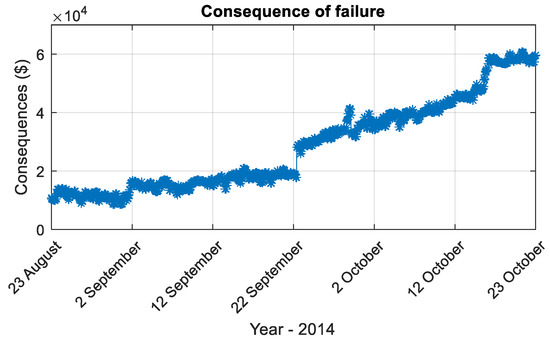
Figure 19.
Consequence of a fault that happened in the compressor.
The system health indicator combined both and . Figure 20 shows the system health indicator of the compressor that was tested for the online phase. and were respectively calculated in offline and online phases, as descripted in Section 2.1.4 and Section 4.2.

Figure 20.
System health indicator presented by risk profile of the compressor.
In this case, the health indicator detected the fault during 22 September to 2 October 2014. Compared to the measured variables obtained from the compressor’s condition monitoring system in Figure 21, during this time, only slight changes appeared in the measurements of the compressor. This indicated that the health indicator successfully detected the fault at its incipient stage.

Figure 21.
Fault relevant variables from the compressor’s condition monitoring system.
In Figure 20, is the shutdown threshold used for system protection. In this case, the company shut down the compressor at 23 October, which is 7 days after the risk value exceeded the shutdown threshold . As can be seen in Figure 21, from 22 September to 16 October, mainly measurements of the stage 3 DE bearing were abnormal. However, after 16 October, many other measurements (i.e., the vibration of the stage 1–2 DE bearing, the vibration of the stage 3 NDE bearing, the suction temperature of stage 2) were influenced by the faulty bearing, which indicated the system was deteriorated and in a dangerous condition. As can be seen in Figure 20 that the developed health indicator suggested to shut down the compressor not later than 16 October, in order to avoid the dangerous condition.
5. Conclusions
In this paper, a system-wide health indicator is proposed using condition monitoring-based dynamic risk assessment, providing maintenance solutions based on real-time health monitoring of assets. The methodology combines two advanced fault detection methods, a sparse autoencoder and robust Mahalanobis distance, which enables the health indicator to detect a fault at its incipient stage and estimate financial loss. The proposed health indictor presents the system’s risk in dollars, making it effective in operational decision-making in a process system. To evaluate the performance of the proposed indicator, two case studies were carried out with multivariate industrial data obtained from a pump and a compressor. The results show that the indicator was able to show the degradation of the system with dynamically updated process risk at each sampling instant. In both cases, the health indicator was able to identify the faults at their incipient stages, before the measured signals showed obvious changes. The fault analysis scheme can analyze the contribution of each measurement, inferring the possible fault types to assist the maintenance planning. Especially in the second case, after the indicator exceeded the suggested shutdown threshold, many other measurements (i.e., the vibration of the stage 1–2 DE bearing, vibration of the stage 3 NDE bearing) were influenced by the faulty bearing, which indicated the system was deteriorated to a dangerous point. In this case, the proposed health indicator suggested appropriate shutdown time before the system suffered severe damage.
The main benefits of the proposed method include early detection of faults, fault analysis, suggesting maintenance time, safety improvement, and minimum interruption of operation. In summary, the main contributions of this paper include:
- (1)
- A system-wide health indicator has been developed using condition-based dynamic risk assessment. The proposed health indictor presented the system’s risk in dollars, making it easier for operators to make maintenance decisions. In addition, the health indicator can demonstrate the health condition of the system to the operator in real time, and assist the operators as to when an incipient fault is detected, how the system is degraded, what type of fault the machine suffers from, and when the deadline is for maintenance.
- (2)
- The probability of a fault is calculated based on the application of a state-of-the-art fault detection models, SAE and MD. To the authors’ knowledge, this is the first time a study has obtained fault probability from a single system-wide feature calculated in MD value, instead of using multiple measurements of a system. Compared with other statistical measurements, such as Hotelling’s and Euclidean distance, the MD is a better way to calculate probability of fault. The value of Hotelling’s is much higher than MD (nearly squared). When using Hotelling’s , the value can increase rapidly to a very high value after a fault appears. This makes a fault more obvious in a fault detection process; however, it is hard to transfer such rapidly changing and highly statistical value to a fault probability. In contrast, the value of Euclidean distance is much more moderate. However, it is not as sensitive as MD for early fault detection in our cases.
- (3)
- The proposed health indicator is evaluated by using a pump and a compressor using multivariate industrial data. This methodology can also be applied to other types of machines’ health assessments, such as turbines and motors. In addition, our experience of processing the industrial data set can benefit relevant readers.
Author Contributions
Conceptualization, X.L. and F.D.; investigation and methodology, X.L. and F.D.; data analysis, X.L.; validation, F.D. and D.M.; writing—original draft preparation, X.L.; writing—review and editing, F.D., D.M., and I.B.; funding acquisition, D.M. All authors have read and agreed to the published version of the manuscript.
Funding
This research received no external funding.
Institutional Review Board Statement
Not applicable. This study does not involve humans or animals.
Informed Consent Statement
Not applicable. This study does not involve humans or animals.
Data Availability Statement
Data sharing is not applicable to this article.
Conflicts of Interest
The authors declare no conflict of interest.
References
- Venkatasubramanian, V.; Rengaswamy, R.; Yin, K.; Kavuri, S.N. A review of process fault detection and diagnosis: Part I: Quatitative model-based methods. Comput. Chem. Eng. 2003, 27, 293–311. [Google Scholar] [CrossRef]
- Liao, G.-L. Optimal economic production quantity policy for randomly failing process with minimal repair, backorder and preventive maintenance. Int. J. Syst. Sci. 2012, 44, 1602–1612. [Google Scholar] [CrossRef]
- Arunraj, N.S.; Maiti, J. Risk-based maintenance—Techniques and applications. J. Hazard. Mater. 2007, 142, 653–661. [Google Scholar] [CrossRef]
- Holland, M.L. Cost savings achievable through application of risk based inspection philosophies. In Risk, Economy and Safety, Failure Minimisation and Analysis Failures ’96, Proceedings of the Second International Symposium, Pilanesberg, South Africa, 22–26 July 1998; Penny, R.K., Ed.; CRC Press: Roca Raton, FL, USA, 1998; p. 8. [Google Scholar]
- Kalantarnia, M.; Khan, F.; Hawboldt, K. Dynamic risk assessment using failure assessment and Bayesian theory. J. Loss Prev. Process. Ind. 2009, 22, 600–606. [Google Scholar] [CrossRef]
- Meel, A.; Seider, W.D. Plant-specific dynamic failure assessment using Bayesian theory. Chem. Eng. Sci. 2006, 61, 7036–7056. [Google Scholar] [CrossRef]
- Kaplan, S.; Garrick, B.J. On the quantitative definition of risk. Risk Anal. 1981, 1, 11–27. [Google Scholar] [CrossRef]
- Yang, M.; Khan, F.I.; Lye, L. Precursor-based hierarchical Bayesian approach for rare event frequency estimation: A case of oil spill accidents. Process Saf. Environ. Prot. 2013, 91, 333–342. [Google Scholar] [CrossRef]
- Khakzad, N.; Khan, F.; Amyotte, P. Dynamic risk analysis using bow-tie approach. Reliab. Eng. Syst. Saf. 2012, 104, 36–44. [Google Scholar] [CrossRef]
- Camci, F.; Medjaher, K.; Atamuradov, V.; Berdinyazov, A. Integrated maintenance and mission planning using remaining useful life information. Eng. Optim. 2018, 51, 1794–1809. [Google Scholar] [CrossRef]
- Hu, C.; Youn, B.D.; Wang, P.; Yoon, J.T. Ensemble of data-driven prognostic algorithms for robust prediction of remaining useful life. Reliab. Eng. Syst. Saf. 2012, 103, 120–135. [Google Scholar] [CrossRef]
- Zio, E. The future of risk assessment. Reliab. Eng. Syst. Saf. 2018, 177, 176–190. [Google Scholar] [CrossRef]
- Zadakbar, O.; Imtiaz, S.; Khan, F. Dynamic risk assessment and fault detection using a multivariate technique. Process Saf. Prog. 2013, 32, 365–375. [Google Scholar] [CrossRef]
- Bao, H.; Khan, F.; Iqbal, T.; Chang, Y. Risk-based fault diagnosis and safety management for process systems. Process Saf. Prog. 2010, 30, 6–17. [Google Scholar] [CrossRef]
- Zadakbar, O.; Imtiaz, S.; Khan, F. Dynamic risk assessment and fault detection using principal component analysis. Ind. Eng. Chem. Res. 2013, 52, 809–816. [Google Scholar] [CrossRef]
- Zadakbar, O.; Khan, F.; Imtiaz, S. Dynamic risk assessment of a nonlinear non-gaussian system using a particle filter and detailed consequence analysis. Can. J. Chem. Eng. 2015, 93, 1201–1211. [Google Scholar] [CrossRef]
- Zeng, Z.; Zio, E. Dynamic risk assessment based on statistical failure data and condition-monitoring degradation data. IEEE Trans. Reliab. 2018, 67, 609–622. [Google Scholar] [CrossRef]
- American Petroleum Institute. A.P.I. 581, Risk-Based Inspection Methodology, 3rd ed.; API: Washington, DC, USA, 2016. [Google Scholar]
- Khan, F.; Wang, H.; Yang, M. Application of loss functions in process economic risk assessment. Chem. Eng. Res. Des. 2016, 111, 371–386. [Google Scholar] [CrossRef]
- Hashemi, S.J.; Ahmed, S.; Khan, F. Risk-based operational performance analysis using loss functions. Chem. Eng. Sci. 2014, 116, 99–108. [Google Scholar] [CrossRef]
- Hashemi, S.J.; Ahmed, S.; Khan, F. Loss functions and their applications in process safety assessment. Process Saf. Prog. 2014, 33, 285–291. [Google Scholar] [CrossRef]
- Yu, H.; Khan, F.; Garaniya, V.; Gareaniya, V. Risk-based process system monitoring using self-organizing map integrated with loss functions. Can. J. Chem. Eng. 2016, 94, 1295–1307. [Google Scholar] [CrossRef]
- Zouari, R.; Sieg-Zieba, S.; Sidahmed, M. Fault detection system for centrifugal pumps using neural networks and neuro-fuzzy techniques. Surveillance 2004, 5, 11–13. [Google Scholar]
- Rajakarunakaran, S.; Venkumar, P.; Devaraj, D.; Rao, K.S.P. Artificial neural network approach for fault detection in rotary system. Appl. Soft Comput. 2008, 8, 740–748. [Google Scholar] [CrossRef]
- Eom, Y.H.; Yoo, J.W.; Bin Hong, S.; Kim, M.S. Refrigerant charge fault detection method of air source heat pump system using convolutional neural network for energy saving. Energy 2019, 187, 115877. [Google Scholar] [CrossRef]
- Gugulothu, N.; Malhotra, P.; Vig, L.; Shroff, G. Sparse neural networks for anomaly detection in high-dimensional time series. In Proceedings of the AI4IOT—Workshop on AI for Internet of Things, Stockholm, Sweden, 13–15 July 2018. [Google Scholar]
- Bokrantz, J.; Tjernberg, L.B. An artificial neural network approach for early fault detection of gearbox bearings. IEEE Trans. Smart Grid 2015, 6, 980–987. [Google Scholar] [CrossRef]
- Bangalore, P.; Letzgus, S.; Karlsson, D.; Patriksson, M. An artificial neural network-based condition monitoring method for wind turbines, with application to the monitoring of the gearbox. Wind Energy 2017, 20, 1421–1438. [Google Scholar] [CrossRef]
- Jiang, G.; Xie, P.; He, H.; Yan, J. Wind turbine fault detection using a denoising autoencoder with temporal information. IEEE/ASME Trans. Mechatron. 2018, 23, 89–100. [Google Scholar] [CrossRef]
- Liang, X.; Duan, F.; Bennett, I.; Mba, D. A sparse autoencoder-based unsupervised scheme for pump fault detection and isolation. Appl. Sci. 2020, 10, 6789. [Google Scholar] [CrossRef]
- Ng, A. Sparse autoencoder. In CS294A Lecture Notes; 2011; Volume 72, pp. 1–19. Available online: http://ailab.chonbuk.ac.kr/seminar_board/pds1_files/sparseAutoencoder.pdf (accessed on 28 November 2020).
- Leys, C.; Klein, O.; Dominicy, Y. Detecting multivariate outliers: Use a robust variant of the Mahalanobis distance. J. Exp. Soc. Psychol. 2018, 74, 150–156. [Google Scholar] [CrossRef]
- Hua, C.; Zhang, Q.; Xu, G.; Zhang, Y.; Xu, T. Performance reliability estimation method based on adaptive failure threshold. Mech. Syst. Signal. Process. 2013, 36, 505–519. [Google Scholar] [CrossRef]
- Feldman, R.M.; Valdez-Flores, C. Applied Probability and Stochastic Processes; Springer Science & Business Media: Berlin/Heidelberg, Germany, 2010. [Google Scholar]
- Wang, H.; Khan, F.; Ahmed, S.; Imtiaz, S. Dynamic quantitative operational risk assessment of chemical processes. Chem. Eng. Sci. 2016, 142, 62–78. [Google Scholar] [CrossRef]
- Deketelaere, B.; Hubert, M.; Schmitt, E. Overview of PCA-based statistical process-monitoring methods for time-dependent, high-dimensional data. J. Qual. Technol. 2015, 47, 318–335. [Google Scholar] [CrossRef]
- Qin, S.J. Survey on data-driven industrial process monitoring and diagnosis. Annu. Rev. Control. 2012, 36, 220–234. [Google Scholar] [CrossRef]
- Mastrangelo, C. Statistical monitoring of complex multivariate processes with applications in industrial process control. J. Qual. Technol. 2013, 45, 118–119. [Google Scholar] [CrossRef]
- Brown, S.; Tauler, R.; Walczak, B. Comprehensive Chemometrics: Chemical and Biochemical Data Analysis, 2nd ed.; Elsevier: Amsterdam, The Netherlands, 2020. [Google Scholar]
- Zhu, X.; Braatz, R.D. Two-dimensional contribution map for fault identification [Focus on Education]. IEEE Control. Syst. 2014, 34, 72–77. [Google Scholar] [CrossRef]
- American Petroleum Institute. API Recommended Practice 581—Risk-Based Inspection Technology, 2nd ed.; API: Washington, DC, USA, 2008. [Google Scholar]
Publisher’s Note: MDPI stays neutral with regard to jurisdictional claims in published maps and institutional affiliations. |
© 2020 by the authors. Licensee MDPI, Basel, Switzerland. This article is an open access article distributed under the terms and conditions of the Creative Commons Attribution (CC BY) license (http://creativecommons.org/licenses/by/4.0/).