Dynamic Approach to Evaluate the Effect of Reducing District Heating Temperature on Indoor Thermal Comfort

Abstract

To reduce energy consumption for space heating, a coordinated action on energy supply, building fabric and occupant behavior is required to realize sustainable improvements. A reduction in district heating supply temperature is an interesting option to allow the incorporation of renewable energy sources and reduce distribution losses, but its impact on the final users must be considered. This aspect is especially critical as most European countries feature an old building stock, with poor insulation and heating systems designed for high-temperature operation. In this study, a complete methodology is devised to evaluate the effect of district heating temperature reduction on the end users by modeling all the stages of the system, from the primary heat exchanger to the indoor environment. A dynamic energy performance engine, based on EN ISO 52016-1:2017 standard and completed with a heat exchanger model, is implemented, and its outputs are used to calculate thermal comfort indicators throughout the heating season. As a practical application, the method is used to evaluate different scenarios resulting from the reduction of primary supply temperature of a second-generation district heating network in Northern Italy. Several building typologies dating back to different periods are considered, in the conservative assumption of radiator heating. The results of the simulations show that the most severe discomfort situations are experienced in buildings built before 1990, but in recent buildings the amount of discomfort occurrences can be high because of the poor output of radiators when working at very low temperatures. Among the possible measures that could help the transition, actions on the primary side, on the installed power and on the building fabric are considered. The investigation method requires a limited amount of input data and is applicable to different scales, from the individual building to entire urban areas lined up for renovation.

1. Introduction

Buildings are a key element in energy and environmental policies worldwide. According to the International Energy Agency [1], despite the increased awareness of governments and population, direct and indirect energy-related CO${}_2$ emissions from buildings have been rising again in the last three years after the encouraging flattening in 2013–2016. With many European countries still lacking mandatory building codes, the benefit in terms of energy savings deriving from renovations of existing buildings should grow from the current 15% to at least 30%–50% to be in line with the sustainable development scenario by 2030 [1]. These figures show that the development of strategies, methodologies and tools are essential to rapidly promote effective upgrades of the current stock.

The need to devise strategies at the urban scale is widely documented in the recent literature. In a 2007 article, Lowe [2] focuses on measures to reduce CO${}_2$ emissions in the UK residential sector, pointing out that the performance of housing is the result of the synergies between the different subsystems, and for a given level of investment the combination of several even modest improvements is likely to produce more benefit than a single major retrofit. The three pillars on which any upgrading approach is based are input data collection, choice of the appropriate calculation method, and identification of relevant indicators. The input information required for the analysis is related, among others, to building details and technical systems. Ballarini et al. [3] present the Italian results of the European project TABULA (Typology Approach for Building Stock Energy Assessment), in which the participants defined the characteristic building typologies of their countries and possible sets of retrofitting measures. A frequently used criterion for the identification of reference buildings is the age of construction as obtained from municipal databases or censuses, as in Di Turi and Stefanizzi [4] and in Delmastro et al. [5]. However, these sources generally do not include information about refurbished buildings, which poses additional challenges to the accurate analysis of the existing building stock [6]. Another possible source of data are energy performance certificates, although some uncertainty in the compilation of the reports must be accepted [7]. The trend is to look for automated data collection methods as in Nageler et al. [8], who propose a methodology to automatically create building models of entire urban districts, based on publicly available datasets and tools, ready to be fed as input to the energy calculation engine. Mutani and Todeschi [9] add urban context parameters by means of a geographic information system (GIS) tool to the calculation model, whereas Torabi Moghadam et al. [10] describe the construction of a GIS database from different sources, including district heating meter data.

Building modeling for energy calculation purpose is the subject of several literature works. Conversely, not many papers focus on the building “circulatory system”: indeed, heating, ventilation, and air conditioning (HVAC) systems are often modeled by assuming the technical equipment typical of the building construction period; however, such models cannot incorporate the variability of the actual installations and the comfort preferences of the occupants [11]. Noussan and Nastasi [12] analyze data from the regional registry of heating plants in Lombardy, Italy, while Mancini and Nastasi [13] adopt a survey approach to collect information about building features, technical services and appliances. Westermann et al. [14] develop a method to automatically infer building type and heating system type from the energy signature, expressed as the electricity consumption for heating and/or cooling detected by smart meters as function of outside temperature recordings.

The evolution of water-based systems points in the direction of reducing supply and return temperatures. It is well known that condensing boilers are fully exploited with low return temperatures, whereas electrically-powered heat pumps work best with low supply temperature systems. Moreover, low-temperature heating systems are associated to lower energy consumption [15], which expands the range of usable sources. In the case of district heating (DH), several benefits can be obtained by lowering the temperature regime. A summary of enabling technologies, best practices and pilot installations for 4th generation DH can be found in the “Guidelines for Low-Temperature District Heating” report [16], from which the amount of variables involved at different scales and the complexity of possible conversion processes emerge. In their work on the optimization of a distributed DH network, Sameti et al. [17] act on piping layout, power flow among the buildings, and type, location, and rated heat and electricity production of generators to minimize the annual cost function, including the cost of CO${}_2$ emissions. The main tool for decarbonization is the integration of renewable energy sources (RES), but this is a challenging task, mainly because of their variability in space and time. Solar energy, for instance, is an abundant source at most European latitudes, but it requires reliable tools to evaluate both the actual energy potential [18] and the correct sizing and operation of the system [19]. The mismatch between demand and supply is usually overcome through flexible-oriented solutions, like the installation of thermal energy storages (TES) [20]). As an example, the long-standing DH system in Brescia, located in Northern Italy, has recently started to incorporate TES and aims to quickly deploy an overall stored energy of 550 MWh, which is estimated to save 1000 toe per year of energy produced by fossil fuels. Another RES-related issue is the correct allocation of the produced energy between fossil and RES share [21], which is important for example with regard to incentivizing policies.

The incorporation of RES is one of the driving forces towards the progressive decrease in the heat transfer medium temperatures. Other benefits associated to this action are the reduction of grid losses [22,23], and the improvement of the powerplant efficiency when the heat is produced in cogeneration facilities (such as in the Brescia municipal system). However, whether this action is feasible (and to which extent) depends on several factors. The installed power and the original design conditions are key elements for the transition to lower temperature systems. Østergaard et al. [24] provide an insight on the radiators installed in Denmark by means of a survey, showing that, as per common belief, most of them are oversized. Tunzi et al. [25] correlate the logarithmic mean temperature difference (LMTD) between the radiator and the surrounding space with the part-load duration, showing that even the radiators sized exactly to fulfill the design heat load are actually oversized for most of the time. Both papers suggest that there is a large potential for low temperature DH with minor or no modification of the building or its internal HVAC systems. Such potential depends strongly on the original design temperatures, which are typical of a specific time period and of a given country. For example, in the 1970s, common design supply/return temperatures for the heating systems were 80/40 ${}^{\circ }$C in Denmark [26] and 75/50 ${}^{\circ }$C in Sweden [27], while 85/75 ${}^{\circ }$C was still common in Italy [28]. Millar et al. [29] investigate the limitations of connecting a traditional 20th century tenement to a low temperature district heating (LTDH). The authors calculate that the minimum supply temperature at the radiator inlet required to meet 80% of the demand is around 85 ${}^{\circ }$C for dwellings with no insulation nor double glazing. They assume common practice radiators’ sizes and design temperatures (82/71/20 ${}^{\circ }$C) similar to those typical in Italy until the 1990s. Their conclusion is that internal improvements are likely to be necessary for the connection to a third generation DH to become a viable option. Likewise, Ashfaq and Ianakiev [30] review the challenges associated to the transition from boiler-base heating to LTDH and, while focusing on the low temperature difference deriving from hydraulic imbalance, they take the need of building retrofitting for granted.

The temperature lowering potential also depends on the type of substation connecting the DH network to the building internal system. When DH is directly connected to the space heating user pipes, the only difference between DH supply temperature and actual temperature at the emitter inlets is caused by thermal losses along the pipe. However, when the user system is separated from DH network by a heat exchanger (indirect connection), the actual radiator supply temperature strongly depends on the type of control and on the characteristics of the heat exchanger. Neirotti et al. [31] explore the effect of reducing DH temperature on a typical North-Italian building with radiator-based heating, comparing two different refurbishing strategies based on continuous operation and on building insulation improvement. They assume a coil heat exchanger modeled by means of a Modelica library component, although DH substations more often use plate heat exchangers.

With regard to the choice of the mathematical modeling framework, given the need to examine transient periods and to incorporate controls and schedules, it is reasonable to opt for a dynamic energy calculation engine. In the past, the level of detail of the models were somehow limited by the available computational capabilities. Crabb et al. [32] develop a single-zone resistor-capacitor (RC) model based on two capacity nodes (indoor air and thermal inertia of the building), which despite its simplicity provides a fair representation of the energy performance of a school. The first international standard including a dynamic hourly model is EN ISO 13790:2008, in which the building is described by five resistors and only one capacitor (5R1C). A validation of the model can be found in the works by Michalak [33]. The EN ISO 13790:2008 was withdrawn in 2017, when it was replaced by the current reference standard for dynamic hourly energy calculations, EN ISO 52016-1:2017 [34], in which the number of resistances and capacitors depends on the geometry and thermal characteristics of the building features and fixtures. The standard is open to the inclusion of other validated methods on a national basis. It is the case of Annex A in the Italian implementation, in which a procedure is provided to calculate the number of nodes of each opaque element instead of the fixed number of layers prescribed by the general framework [35]. The EN ISO 52016-1:2017 has multiple usages: it is the common platform for energy calculation softwares and for national building regulations; it can be employed as a tool to validate other methods (see for instance Campana and Morini [36]); it provides a complete calculation framework that can serve as a basis to build affordable codes. In a recent paper, Lundström et al. [37] introduced some simplifications to the EN ISO 52016-1:2017 building model, with the aim of reducing the complexity of input data and the required computational effort. Their focus is the supervision of thousands of dwellings by few managers, who must be able to quickly construct the building model and run swift simulations to identify present and potential energy performances. An alternative to physical modeling is represented by gray box [38] or black box [39] approaches, which nowadays can rely on increasing amounts of available information, on a wide range of efficient algorithms and on improved performances of calculation machines. Open models and data are expected to play a key role in the development of new energy-related methodologies [40].

The final stage of the analysis is the definition of performance indicators to quantitatively evaluate and compare different scenarios. As pointed out by Tronchin et al. [41], an effective energy modeling strategy should feature modularity and possibility of representation across multiple scales, including the user perspective. The classical approach to indoor comfort was developed by Fanger in the 1970s and relies upon the calculation of parameters such as predicted mean vote (PMV) and predicted percentage of dissatisfied (PPD), whose formulations have been included in standards worldwide, such as ANSI/ASHRAE 55 and EN ISO 7730. Derived long-term indices are the number of discomfort hours, used for example in the work by Braulio-Gonzalo et al. [42] to analyze the indoor thermal comfort of residential building stocks, and percentage outside range (POR), among the several indices compared by Carlucci et al. [43] in the cooling assessment of office building variants. Stasi et al. [44] use PMV, PPD and POR for the evaluation of indoor comfort of a nearly zero-energy building in Southern Italy. References [42,43,44] all derive the comfort indices from dynamic energy simulations.

To summarize, the scientific and technical literature features dynamic energy calculation models, studies on the collection and processing of the required input data, and indoor thermal comfort assessment methodologies and case studies. The theoretical applicability of LTDH to existing buildings is also discussed in several papers, but with some limitations in primary/secondary interface modeling and with results mainly presented in terms of temperature variations. To the best of the authors’ knowledge, no large-scale dynamic analysis of a building-thermal systems complex has been carried out that includes an accurate model of the primary heat exchanger and a quantitative estimation of the occupants’ comfort response. The aim of the present study is to devise a complete methodology to assess the impact of DH supply temperature reduction on the indoor thermal comfort in existing buildings, including a detailed model of the DH heat exchanger and expressing the results in terms of thermal comfort indices. A practical application is presented to demonstrate the potential of the method on buildings connected a typical Northern Italian DH network. The evaluation is extended to the buildings stock of the selected area, to represent which the Italian reference building matrix elaborated in the TABULA project is used. The main assumptions in this application are the indirect connection of the user heating system to the DH through a heat exchanger and the presence of radiator-based user heating systems, being this type of emitter more critical than low-temperature radiant panel heating from the viewpoint of supply temperature reduction.

The paper is organized as follows. Section 2 summarizes the modules composing the proposed simulation framework. In particular, the dynamic model recently proposed by Lundström et al. [37] has been chosen as a central energy calculation engine. Primary heat exchanger and radiator heating system models are also described in this Section. The application of the method is presented in Section 3, where the climate-related input data, the heating system, the building typology matrix, and the selected comfort performance indices are described. The results and discussion are reported in Section 4, followed by conclusions and future developments in Section 5.

2. Methodology

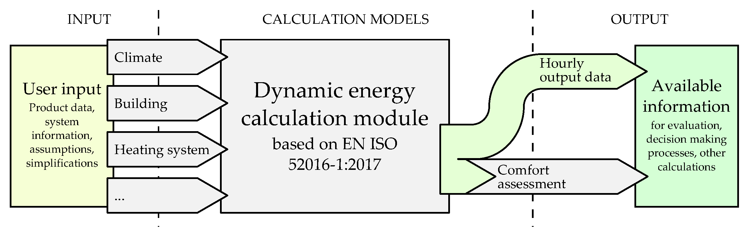
2.1. Calculation Framework

The proposed method relies upon the modular structure represented in Figure 1, whose center is the energy calculation model. The model takes as input climate information, building details and heating system preferences, and provides time-dependent output information that can be used for energy consumption, performance and comfort evaluations. Several calculation options are available to perform different tasks—for example, the user can simulate free-floating operation, operation with ideal heating/cooling (thermostat) or with actual heating/cooling systems.

Input data are provided in two ways:

• A text general input file, in which the main settings and input parameters are listed, and
• Database spreadsheet files for buildings and primary heat exchangers

The code is developed in MATLAB.

2.2. Energy Calculation Model

To calculate the energy balance of the building, the approach proposed by Lundström et al. [37] is chosen. The model is largely based on the dynamic hourly method of EN ISO 52016-1:2017, the main difference being that all the elements of the same type (for example external walls) are lumped into a single element. Moreover, each opaque element is modeled with only three layers, with respect to the five prescribed by the standard. These simplifications lead to a building model with a fixed number of nodes (14, hence the model name “ISO14N” adopted by the authors), which greatly reduces the complexity of the required input data. ISO14N is developed for a single thermal zone. The calculation matrix, tying the previous time-step values to the present time-step outputs, is compiled following the EN ISO 52016-1:2017 approach, that is, by writing the heat balances for the thermal zone and its different elements. In the balances for the external surface nodes, where radiant heat gains depend upon surface orientation, the actual expositions of the elements are considered by calculating average irradiances weighted for the fractions of the overall surface exposed at different angles. In Reference [37], building simulation software IDA ICE is used to validate the method. In the present work, an additional comparison between the results obtained from ISO14N code, EN ISO 52016-1:2017 supporting calculation sheets, and EnergyPlus software for the reference BESTest cases provided by EN ISO 52016-1:2017 standard is reported in the Supplementary Materials, where the statistical indices described in Reference [45] are used to evaluate the prediction capabilities of the simplified approach.

In the study presented in the original paper in Reference [37], a model was included for a radiator-based heating system, which is illustrated and expanded in the next Subsection.

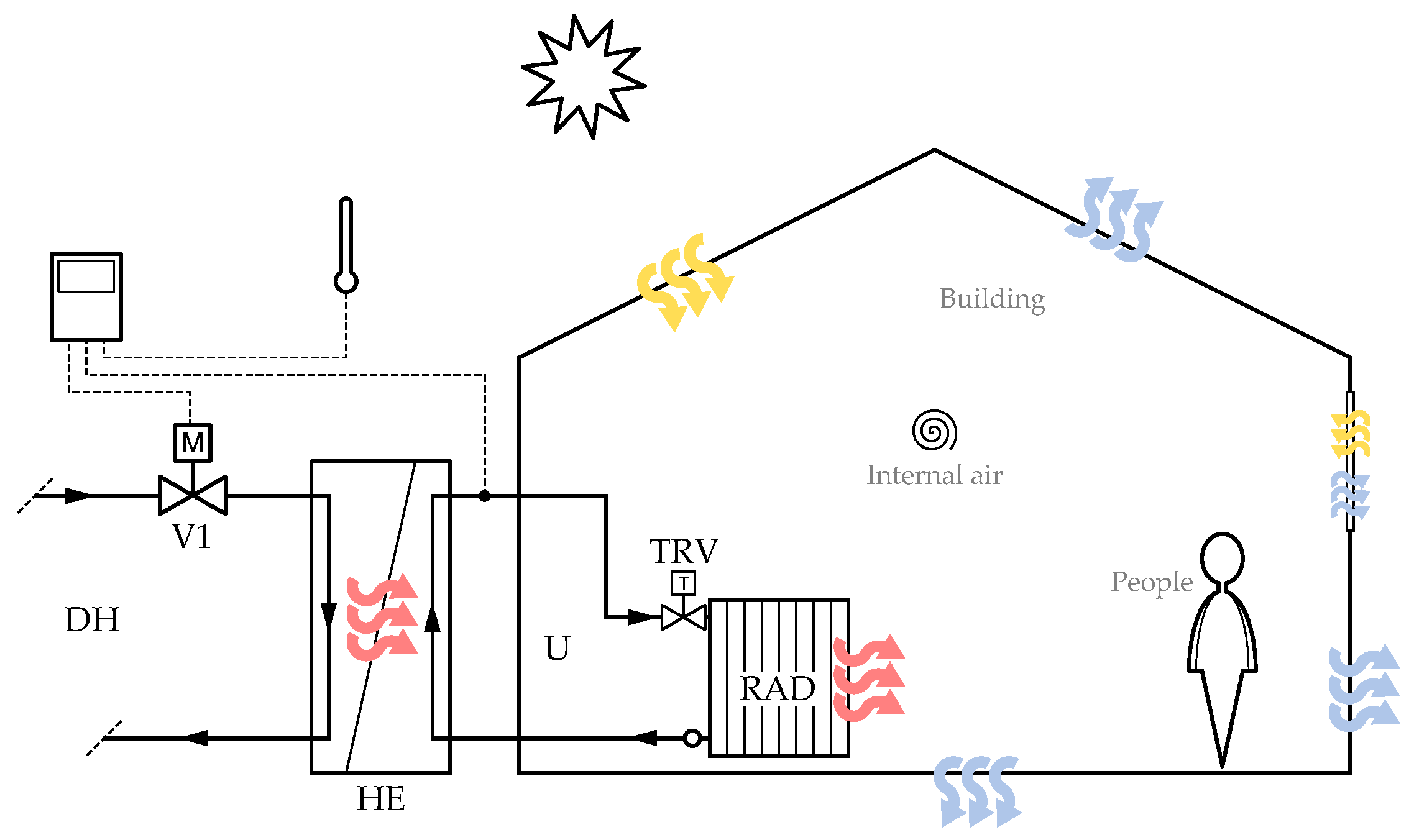
2.3. Heating System Model

The indirect connection between DH and user system is modeled in this paper according to the most common configuration in Italy, sketched in Figure 2, that is, by means of a plate heat exchanger. Hence, the base configuration assumes the following equipment:

• Plate heat exchanger (HE) to transfer heat from the primary (DH) side to the secondary (user, U) side; it is modeled based on the technical information provided by the manufacturer, as explained below.
• Primary control valve (V1), to modulate the primary flow rate in order to obtain the desired supply temperature on the secondary side; it is assumed as an ideal component that instantaneously performs the required action.
• Thermostatic radiator valve (TRV), a proportional controller that modulates the secondary flow rate according to the difference between room temperature and average radiator temperature.
• Radiator (RAD) with a given nominal power referred to the design temperatures typical of the period of installation; due to the single-zone assumption, all the heating emitters are lumped into a single component, whose installed power is calculated in a preliminary simulation run based on the peak load of the building.

The primary control valve can be associated with either weather-compensated or fixed-point control, according to the user preferences. In the former case, the heating curve relating the secondary supply temperature to the outdoor temperature must be set, whereas only a fixed value is required in the latter case. It is worth noting that no hydraulic calculation is performed on the primary or the secondary circuit. However, a maximum flow rate can be set for both sides, to simulate the maximum capacity of a pump.

The following equations describe the whole heating system model. They are listed starting from the room and backwards to the DH network.

Power released to the room. The equation describing the heat release $\mathsf{\Phi }$ from a radiator with thermostatic control to the room is

$$\mathsf{\Phi }={\mathsf{\Phi }}_{\mathrm{nom}}\times {\left(\frac{\mathsf{\Delta }\theta }{\mathsf{\Delta }{\theta }_{\mathrm{nom}}}\right)}^{{\mathit{n}}_{\mathrm{rad}}}\times u_{\mathrm{TRV}},$$

(1)

where ${\mathsf{\Phi }}_{\mathrm{nom}}$ is the nominal thermal power referred to the conditions expressed by the nominal logarithmic mean temperature difference (LMTD) $\mathsf{\Delta }{\theta }_{\mathrm{nom}}$, and $n_{\mathrm{rad}}$ is the characteristic exponent of the radiator. $u_{\mathrm{TRV}}$ is the modulation factor introduced by the action of a thermostatic valve with proportional band $PB$:

$$u_{\mathrm{TRV}}=max\left\{0,min\left\{1,\left({\theta }_{\mathrm{ref},\mathrm{set}}-{\theta }_{\mathrm{ref},\mathit{t}-1}\right)/PB\right\}\right\}.$$

(2)

$\mathsf{\Delta }\theta$ is the actual LMTD between the radiator mean temperature and the room, calculated at each time step and given by

$$\mathsf{\Delta }\theta =\frac{{\theta }_{\mathrm{u},\mathrm{s}}-{\theta }_{\mathrm{u},\mathrm{r}}}{ln\left({\theta }_{\mathrm{u},\mathrm{s}}-{\theta }_{\mathrm{ref},\mathit{t}-1}\right)-ln\left({\theta }_{\mathrm{u},\mathrm{r}}-{\theta }_{\mathrm{ref},\mathit{t}-1}\right)},$$

(3)

where ${\theta }_{\mathrm{u},\mathrm{s}}$ and ${\theta }_{\mathrm{u},\mathrm{r}}$ are the supply and return temperatures of the radiator at the current time step, and ${\theta }_{\mathrm{ref},\mathit{t}-1}$ is the reference internal temperature at the previous time step. Either the air or the operating temperature, defined as the arithmetic average of air and mean radiant temperatures, can be taken as reference internal temperature. The latter option has been chosen in this work.

Return temperature. In their paper, Lundström et al. [37] include an empirical correlation for the return temperature from the radiator which has also been used in the present work:

$${\theta }_{\mathrm{u},\mathrm{r}}={\theta }_{\mathrm{u},\mathrm{s}}-b·{\left({\theta }_{\mathrm{u},\mathrm{s}}-{\theta }_{\mathrm{ref},\mathit{t}-1},\right)}^{\mathit{a}}$$

(4)

where a and b are functions of the nominal supply, return and reference internal temperatures and of the radiator exponent. Other equations are available in the literature, in which the dependencies on other quantities like instantaneous flow rate and radiator inertia are also taken into account (see for example Teskeredzic and Blazevic [46]).

Secondary supply temperature control. The secondary supply temperature is controlled through the modulation of the primary flow rate according to a certain logic. In case of fixed-point option, the control system acts to keep the secondary supply temperature at the set value, ${\overline{\theta }}_{\mathrm{u},\mathrm{s}}$:

$${\theta }_{\mathrm{u},\mathrm{s}}={\overline{\theta }}_{\mathrm{u},\mathrm{s}}.$$

(5)

In the case of outdoor temperature reset, the secondary supply temperature set-point is a function of the current external temperature, ${\theta }_{\mathrm{e}}$, via a heating curve:

$${\theta }_{\mathrm{u},\mathrm{s}}=f\left({\theta }_{\mathrm{e}}\right).$$

(6)

Radiator energy balance. Neglecting the thermal inertia of the radiator, the heating power transferred from the water flowing through the radiator is given by

$$\mathsf{\Phi }={\dot{m}}_{\mathrm{u}}·c_{\mathrm{w},\mathrm{u}}·\left({\theta }_{\mathrm{u},\mathrm{s}}-{\theta }_{\mathrm{u},\mathrm{r}}\right),$$

(7)

where ${\dot{m}}_{\mathrm{u}}$ is the water flow rate through the radiator and $c_{\mathrm{w},\mathrm{u}}$ the specific heat of the water circulating on the user side.

Power supplied by DH. Neglecting the thermal inertia of the water circulating on the user side, the heating power transferred from the DH to the secondary side of the heat exchanger is

$$\mathsf{\Phi }={\dot{m}}_{\mathrm{DH}}·c_{\mathrm{w},\mathrm{DH}}·\left({\theta }_{\mathrm{DH},\mathrm{s}}-{\theta }_{\mathrm{DH},\mathrm{r}}\right),$$

(8)

where ${\dot{m}}_{\mathrm{DH}}$ is DH flow rate and $c_{\mathrm{w},\mathrm{DH}}$ is the specific heat of water on the primary side. In this simplified model, the heat losses through the secondary distribution network have been neglected, therefore, the heat output from the DH interface is equal to the heat output from the radiator. For a general analysis and for comparative studies like the one proposed in this paper, this set of assumptions is considered acceptable. However, if a real building is to be simulated, one might deem appropriate to include heat losses and inertia of the user distribution piping network, and inertia of the room radiators.

DH heat exchanger model. To close the system, a set of equations must be derived that represents the heat transfer behavior of the interface heat exchanger. This model is fully described in the next Subsection.

According to the type of calculation required, these equations can be rearranged to obtain the desired outputs in the light of the given inputs. For example, if no limit is set to the primary flow rate (or if the calculated primary flow rate is below the set limit), the secondary supply temperature is an input and the primary flow rate is an output of the simulation. However, if the calculated primary flow rate exceeds the upper limit, the calculation is repeated taking the maximum primary flow rate as an input and the secondary supply temperature as an output.

2.4. Heat Exchanger Model

The most common heat exchangers that can be found in DH-supplied dwellings in Italy are of plate type. Gasketed heat exchangers feature a frame in which a pack of thin metal sheet plates are sandwiched between gaskets and pressed together by cover plates and bolts. This type of plate heat exchanger is particularly common in apartment blocks, where the possibility to disassemble the device to replace only the damaged parts is an economic advantage. For smaller installations, such as single family houses, brazed-plate heat exchangers are frequently encountered because they are more compact and relatively cheap. In both cases, each plate features a corrugation obtained by stamping a given surface pattern on the metal sheet. The corrugations are essential for many reasons. Besides making the plates more rigid, the corrugations of consecutive plates result in the formation of the flow channels in patterns studied so to promote high heat transfer coefficients while reducing the risk of clogging (fouling). Different types of corrugations are constantly being developed by manufacturers, like the very popular “chevron-type” pattern.

In the present analysis, a rating (or performance) calculation is required. Therefore, an effectiveness-number of transfer units model ($\epsilon$-$NTU$) is chosen, where the exchanged power is expressed as a function of the inlet temperatures [47]:

$$\mathsf{\Phi }=\epsilon ·C_{\min }·\left({\theta }_{\mathrm{DH},\mathrm{s}}-{\theta }_{\mathrm{u},\mathrm{r}}\right),$$

(9)

where $C_{\min /\max }=min/max\{{\dot{m}}_{\mathrm{DH}}{c}_{\mathrm{w},\mathrm{DH}};{\dot{m}}_{\mathrm{u}}{c}_{\mathrm{w},\mathrm{u}}\}$. The effectiveness parameter $\epsilon$ represents the ratio between the actual exchanged power and the maximum power that can be theoretically exchanged given the two temperature endpoints (primary hot inlet and secondary cold inlet). The effectiveness can be written as a function of two parameters: the number of heat transfer units, $NTU$, and the ratio between heat capacity rates of the two streams, R:

$$NTU=\frac{U·A}{C_{\min }}R=\frac{C_{\min }}{C_{\max }},$$

(10)

where A is the overall heat transfer surface and U is the overall heat transfer coefficient:

$$U={\left(\frac{1}{h_{\mathrm{h}}}+\frac{1}{h_{\mathrm{c}}}+\frac{{\delta }_{\mathrm{p}}}{k_{\mathrm{p}}}+R_{\mathrm{foul},\mathrm{h}}+R_{\mathrm{foul},\mathrm{c}}\right)}^{-1}.$$

(11)

In this expression, $h_{\mathrm{h}}$ and $h_{\mathrm{c}}$ are the heat transfer coefficients of the hot and cold flows, ${\delta }_{\mathrm{p}}$ is the plate thickness and $k_{\mathrm{p}}$ its thermal conductivity, while $R_{\mathrm{foul},\mathrm{h}}$ and $R_{\mathrm{foul},\mathrm{c}}$ are the additional resistances introduced by the possible fouling of the plates on the hot (subscript “h”) and cold (subscript “c”) side, respectively. In case of new or well-maintained exchangers, the fouling resistances are set to zero.

Several studies in the literature provide empirical correlations for the estimates of these parameters, based on experimental data available for specific commercial products (see for instance the review in [47], chapter 7). Recently, methods based on artificial neural networks have been proposed which could be particularly interesting when very large amount of data are available (see for example Longo et al. [48]). In the framework of the present analysis, the system of equations is closed by a Dittus-Boelter type correlation [49] as a function of the channel-based Reynolds number $\mathrm{Re}$ and the Prandtl number $\mathrm{Pr}$ of the flow:

$$\mathrm{Nu}=c1·{\mathrm{Re}}^{\mathit{c}2}·{\mathrm{Pr}}^{\mathit{c}3},$$

(12)

where

$$\mathrm{Nu}=\frac{h}{k/d}$$

(13)

is the Nusselt number, that is, the ratio between convective heat transfer, embodied by heat transfer coefficient h, and conductive heat transfer, represented by the fluid conductivity k divided by a characteristic length d. Combining Equations (12) and (13), one obtains for the heat transfer coefficient in the i-th channel:

$$h_{\mathit{i}}=c1·\left(\frac{h_{\mathit{i}}}{d}\right)·{\left(\frac{{\rho }_{\mathit{i}}{u}_{\mathit{i}}d}{{\mu }_{\mathit{i}}}\right)}^{\mathit{c}2}·{\left(\frac{{\mu }_{\mathit{i}}{c}_{\mathrm{w},\mathit{i}}}{k_{\mathit{i}}}\right)}^{\mathit{c}3}.$$

(14)

The key parameters to be estimated in each channel are $u_{\mathit{i}}$ and d. The flow velocity $u_{\mathrm{i}}$ can be expressed as a function of the flow rate once the channel area is obtained from the manufacturer. The characteristic length d is the equivalent diameter defined as $4·WH/[2·(W+H\left)\right]\approx 2·H$, where W is the useful plate width and H the inter-plate height, which can be estimated from the channel area and the number of channels of the considered side. The latter can be found by the number of plates, $n_{\mathrm{p}}$, which is usually even: therefore, one side has $n_{\mathrm{p}}/2$ channels (cold fluid side) and the other side $n_{\mathrm{p}}/2-1$ channels (hot fluid side). This is the preferred configuration because the channels flown through by the hot fluid are separated from the surrounding environment by the two external cold fluid channels, thus the heat losses are limited.

The tuning parameters of the model are $c1$, $c2$ and $c3$ in Equation (14), which should be obtained for every real heat exchanger by fitting experimental data and/or simulation results from advanced proprietary software that manufacturers often make available for their customers.

2.5. Evaluation of Indoor Comfort

EN 16798-1:2019 recently replaced EN 15251:2007 as the reference standard for the parameters required to design and assess the indoor air quality of a building. The standard prescribes that the design criteria for any mechanically conditioned environment be established through comfort indices PMV (predicted mean vote) and PPD (predicted percentage of dissatisfied), described in EN ISO 7730:2005. This comfort assessment model is known as “PMV/PPD”, “static”, or “heat balance” model.

The PMV is an index predicting the mean value of the votes given by a large number of people in a thermal sensation scale ranging from $-3$ (cold) to $+3$ (hot), neutrality being at 0. The formula for PMV is obtained from the thermal balance for the human body, thus it is a function of several input parameters:

• metabolic rate M, expressing a typical level of activity of the occupants;
• thermal insulation for clothing, $I_{\mathrm{cl}}$;
• internal air temperature, ${\theta }_{\mathrm{air}}$;
• mean radiant temperature of the internal surfaces, ${\theta }_{\mathrm{mr}}$;
• air velocity, $v_{\mathrm{air}}$;
• relative humidity, RH.

$$PMV\left(t\right)=f\left(M,I_{\mathrm{cl}},{\theta }_{\mathrm{air}},{\theta }_{\mathrm{mr}},v_{\mathrm{air}},\mathrm{RH}\right).$$

(15)

The PPD index is a function of the sole PMV index representing the percentage of thermally dissatisfied people that can be expected. Once the PMV and/or the PPD for a given condition have been calculated, they must be compared to acceptability limits. These are given by the so-called indoor environmental quality (IEQ) classes (

Table 1. Indoor environmental quality classes and relative index limits ($v_{\mathrm{air}}<0.1$ m/s; RH ≈ 50%; $I_{\mathrm{cl}}\approx 1$ clo).

Category	Level of Expectation	Accepted PMV	Accepted PPD	Minimum ${\mathit{\theta }}_{\mathbf{op}}$ (Heating)
I	High	<6	$-0.2<$ PMV $<+0.2$	$21.0$
II	Medium	<10	$-0.5<$ PMV $<+0.5$	$20.0$
III	Moderate	<15	$-0.7<$ PMV $<+0.7$	$18.0$
IV	Low	<25	$-1.0<$ PMV $<+1.0$	$16.0$

). If used for design purposes, the limit comfort indices for the selected class allow to determine a range of design operative temperatures, ${\theta }_{\mathrm{op}}$.

For long-term evaluation of the comfort conditions, individual index values can be conveniently aggregated [43]. The simplest aggregation can be made by calculating the percentage of hours during which the PMV is outside the comfort range.

It is worth mentioning that a possible alternative (or complementary) approach to evaluate indoor thermal comfort is the application of adaptive methodologies linking the indoor comfort temperature to the outdoor running mean temperature. This category of methods account for the ability of people to adapt to the environment over time, thus coming to accept lower indoor temperatures in winter and higher indoor temperatures in summer with respect to the static approach. They were first introduced in the 1970s for “free running” (or “naturally ventilated”) buildings, in which the occupants have direct control over their environment. An adaptive model is also included in EN 16798-1:2019 standard.

3. Application

3.1. Presentation of the Case

The methodology outlined in the previous Section has been applied to a practical assessment instance. First of all, the location is identified to provide the energy calculation core described in Section 2.2 with the required climate-related input data. Relevant characteristics of the DH network and of the user heating systems, such as working temperature, installed heating power, and heat exchanger features are also collected to fill the input file and the component database. The buildings to simulate are fully described starting from the TABULA typology matrix with the addition of mass distribution, heat capacity, and heating system design information.

Once the input files are completed, the dynamic simulation is run over a year and all the outputs described in EN ISO 52016-1:2017 are obtained. Among these, the hourly indoor air and mean radiant temperatures are extracted and fed as input to the comfort assessment module, and other quantities provided by the dynamic hourly calculation, such as heating system flow rates, supply temperatures and return temperatures, are stored for further analysis.

Details on input information, main assumptions, and calculation choices are given below.

3.2. Heating System Information

According to the 2019 annual report on Italian district heating networks [50], the extension of urban heating distribution network has reached 4446 km, over 95% of which are in Northern Italy. Heat-only boiler stations and cogeneration facilities based on burning fossil fuels, biomass, and urban wastes are the most common types of DH power stations, occasionally in combination with geothermal/groundwater, heat pumps, industrial heat recovery and, more rarely, solar generation systems. Among these, only a few systems operate with wintertime supply temperatures around 70 ${}^{\circ }$C, almost half of the networks operate around 90 ${}^{\circ }$C, and the other half above 110 ${}^{\circ }$C. This study focuses on the city of Brescia, characterized by the second largest DH network in Italy after Turin. Based on declared data, the DH supply temperature is assumed to be 115 ${}^{\circ }$C.

Multiple buildings have been analyzed (see next Subsection) and a heat exchanger had to be assigned to each of them to perform the calculations. The heat exchanger database has been built according to the following steps:

• Full definition of the building.
• Calculation of heating load according to EN ISO 52016-1:2017, clause 6.5.5.2.
• Definition of user supply/return temperatures based on period of construction, which are set as the outlet and inlet flow temperatures on the secondary side of the heat exchanger.
• Calculation of design user flow rate from the calculated load and temperature difference: the secondary side of the heat exchanger is fully characterized.
• Sizing of the heat exchanger with the complete information on the secondary side and the DH supply temperature on the primary side: the DH return temperature and the primary flow rate are outputs of the calculation, together with the heat exchanger model. Here, this step is entirely performed by means of the proprietary software made available by the heat exchanger manufacturer.
• Collection of the heat exchanger parameters necessary for the model described in Section 2.4, including number of plates, heat transfer area, channel areas and so on. Parameters $c1$, $c2$ and $c3$ in Equation (12) are derived by fitting the equation on the results of simulations performed with the manufacturer software.

The heat exchanger database comes in the form of a plain spreadsheet. New plate heat exchangers can seamlessly be added, which are recalled by the building entries in the building database through a unique identifier.

Although the code allows to set a heating curve to simulate the outdoor temperature reset control of the user supply temperature, the simulations in this application case are performed assuming a fixed-point control. This choice is motivated by the need to clearly identify the impact of the DH supply temperature variation without introducing further overlapping effects. Similarly, continuous operation is assumed for the heating system with no night time set-back. As concerns the thermostatic radiator valve, a proportional band $PB=1.0$ K has been assumed in the calculations. The radiator characteristic exponent $n_{\mathrm{rad}}$ has been set to 1.3.

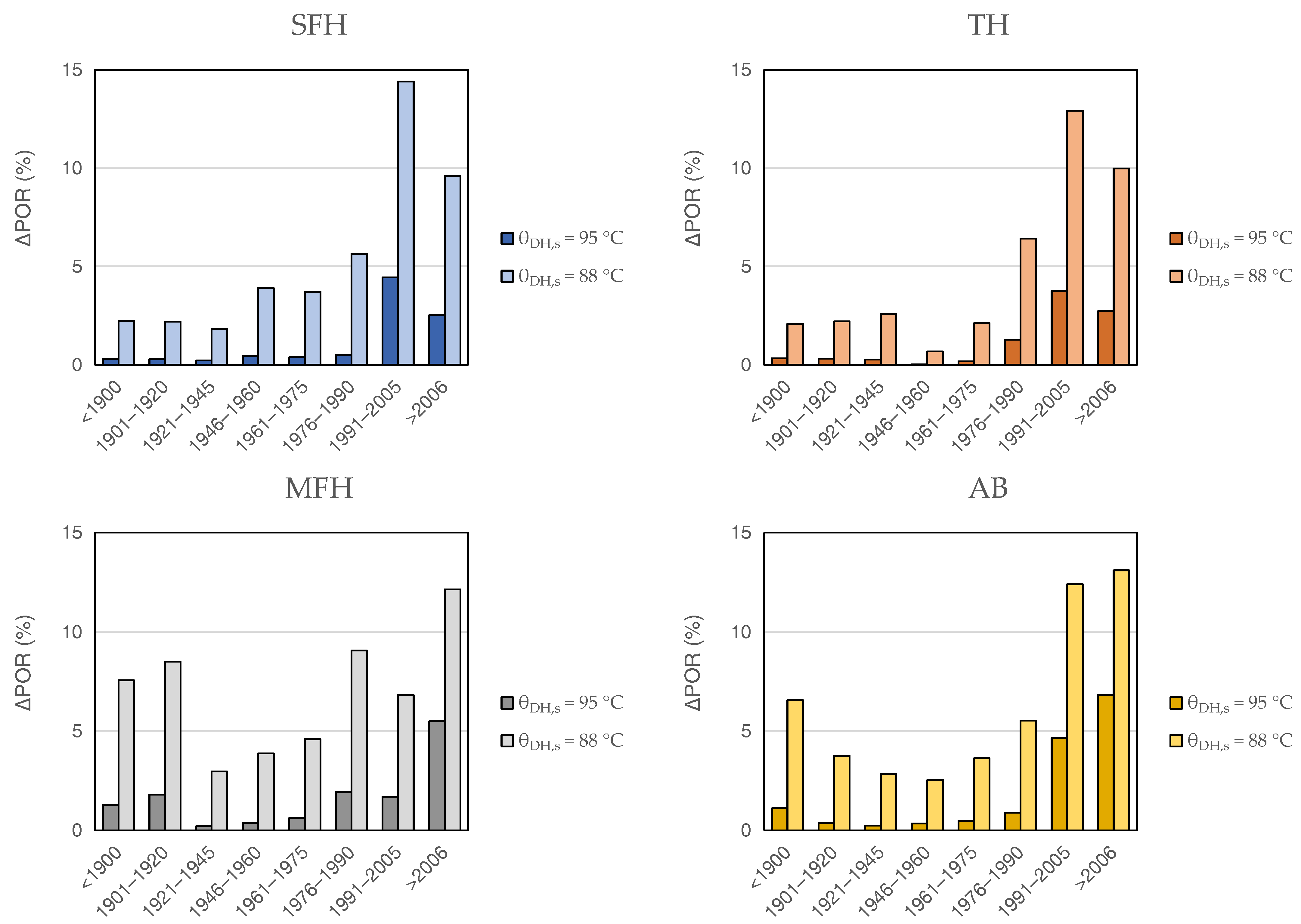
3.3. Building Typology Matrix and Additional Data

To show the potential of the calculation framework even on a large scale, the whole Italian building stock as represented by the Italian building typology matrix developed in the framework of the IEE-TABULA project [3] and of its follow-up IEE-EPISCOPE [51] has been considered. The matrix, originally built based on the analysis of Piedmont region data, well represents the building stock of Italian middle climatic zone, including most of Lombardy region and the city of Brescia in particular. The matrix defines four types of buildings:

• single family house (SFH)
• terraced house (TH)
• multifamily house (MFH)
• apartment block (AB)

and describes them as a function of eight periods of construction:

• ≤1900
• 1901–1920
• 1921–1945
• 1946–1960
• 1961–1975
• 1976–1990
• 1991–2005
• ≥2006

Therefore, each building typology can be identified by a type/period pair. For example, SFH.05 will indicate a single family house built between 1961 and 1975. No renovations are considered in the baseline matrix.

In the TABULA/EPISCOPE project, the energy performances of the buildings were assessed through the quasi-steady monthly model of the Italian reference standards, the UNI/TS 11300 set of standards. Therefore, most of the necessary information is given in the national deliverables of the project [52], such as heated volumes, floor areas, and U-values. However, some additional data are required to perform dynamic hourly calculations with a EN ISO 52016-1-based tool:

• mass distribution of opaque and ground floor elements (

  Table 2. Additional information for the Italian building typology matrix (MDc: mass distribution class, according to Reference [37], Table 1; SHCc: specific heat capacity class, according to Reference [34], Table A.14). Subscripts “rf”, “ew” and “gf” indicate roof, external walls and ground floor elements, respectively.

  Quantity	Unit	SFH.01	SFH.02	SFH.03	SFH.04	SFH.05	SFH.06	SFH.07	SFH.08
  SHCc${}_{\mathrm{rf}}$	-	VL	VL	VL	H	H	H	VH	VH
  MDc${}_{\mathrm{rf}}$	-	E	E	E	M	M	M	D	IE
  SHCc${}_{\mathrm{ew}}$	-	VH	VH	VH	VH	VH	VH	VH	VH
  MDc${}_{\mathrm{ew}}$	-	D	D	D	D	D	IE	M	I
  SHCc${}_{\mathrm{gf}}$	-	VH	VH	VH	VH	VH	VH	VH	VH
  MDc${}_{\mathrm{gf}}$	-	D	D	D	D	D	D	D	E
  ${\theta }_{\mathrm{u},\mathrm{s},\mathrm{nom}}$	${}^{\circ }$C	85	85	85	85	85	75	70	60
  ${\theta }_{\mathrm{u},\mathrm{r},\mathrm{nom}}$	${}^{\circ }$C	75	75	75	75	75	65	55	40
  ${\mathsf{\Phi }}_{\mathrm{nom}}$	W	20,280	18,120	16,630	20,710	22,280	11,870	7000	4480
  Quantity	Unit	TH.01	TH.02	TH.03	TH.04	TH.05	TH.06	TH.07	TH.08
  SHCc${}_{\mathrm{rf}}$	-	VL	VL	VH	H	VH	VL	VH	VH
  MDc${}_{\mathrm{rf}}$	-	E	E	E	M	D	E	IE	IE
  SHCc${}_{\mathrm{ew}}$	-	VH	VH	VH	H	VH	H	VH	VH
  MDc${}_{\mathrm{ew}}$	-	D	D	D	IE	D	IE	M	I
  SHCc${}_{\mathrm{gf}}$	-	H	VH	VH	VH	VH	VH	VH	VH
  MDc${}_{\mathrm{gf}}$	-	D	D	D	D	D	D	IE	E
  ${\theta }_{\mathrm{u},\mathrm{s},\mathrm{nom}}$	${}^{\circ }$C	85	85	85	85	85	75	70	60
  ${\theta }_{\mathrm{u},\mathrm{r},\mathrm{nom}}$	${}^{\circ }$C	75	75	75	75	75	65	55	40
  ${\mathsf{\Phi }}_{\mathrm{nom}}$	W	12,310	11,400	9400	9960	7830	6690	4510	3500
  Quantity	Unit	MFH.01	MFH.02	MFH.03	MFH.04	MFH.05	MFH.06	MFH.07	MFH.08
  SHCc${}_{\mathrm{rf}}$	-	H	VL	VH	VH	VH	VH	VH	VH
  MDc${}_{\mathrm{rf}}$	-	D	D	D	D	D	D	IE	IE
  SHCc${}_{\mathrm{ew}}$	-	VH	VH	VH	VH	H	H	H	VH
  MDc${}_{\mathrm{ew}}$	-	D	D	D	D	IE	M	IE	M
  SHCc${}_{\mathrm{gf}}$	-	H	VH	VH	VH	VH	VH	VH	VH
  MDc${}_{\mathrm{gf}}$	-	D	D	D	D	D	D	IE	IE
  ${\theta }_{\mathrm{u},\mathrm{s},\mathrm{nom}}$	${}^{\circ }$C	85	85	85	85	85	75	70	60
  ${\theta }_{\mathrm{u},\mathrm{r},\mathrm{nom}}$	${}^{\circ }$C	75	75	75	75	75	65	55	40
  ${\mathsf{\Phi }}_{\mathrm{nom}}$	W	51,000	70,090	94,330	63,200	61,620	46,150	34,660	18,750
  Quantity	Unit	AB.01	AB.02	AB.03	AB.04	AB.05	AB.06	AB.07	AB.08
  SHCc${}_{\mathrm{rf}}$	-	VL	VH	VH	VH	VH	VH	VH	VH
  MDc${}_{\mathrm{rf}}$	-	D	D	E	D	D	D	IE	IE
  SHCc${}_{\mathrm{ew}}$	-	VH	VH	VH	H	H	H	VH	VH
  MDc${}_{\mathrm{ew}}$	-	D	D	D	IE	IE	IE	M	M
  SHCc${}_{\mathrm{gf}}$	-	VH	VH	VH	VH	VH	VH	VH	VH
  MDc${}_{\mathrm{gf}}$	-	D	D	I	D	D	D	IE	IE
  ${\theta }_{\mathrm{u},\mathrm{s},\mathrm{nom}}$	${}^{\circ }$C	85	85	85	85	85	75	70	60
  ${\theta }_{\mathrm{u},\mathrm{r},\mathrm{nom}}$	${}^{\circ }$C	75	75	75	75	75	65	55	40
  ${\mathsf{\Phi }}_{\mathrm{nom}}$	W	52,550	224,740	139,630	116,810	164,000	123,030	93,170	46,160

  ). The reference is Table 1 in Lundström et al. [37], where five possible arrangements of the three layers are outlined: mass on interior side (I), mass on exterior side (E), mass divided on interior and exterior side (IE), equally distributed mass (D) and inside/centered mass (M);
• specific heat capacities of opaque and ground floor elements (Table 2). The reference is Table A.14 of EN ISO 52016-1:2017 standard, where five classes are identified: very light (VL), light (L), medium (M), heavy (H), very heavy (VH). The assigment has been made based on the detailed layer structure description given in the TABULA/EPISCOPE project;
• exposition fractions (

  Table 3. Fraction of vertical elements exposed to South, West, East and North.

  Element	South	West	East	North
  External walls	0.3	0.2	0.2	0.3
  Glazing (SFH, MFH, AB)	0.4	0.3	0.3	0
  Glazing (TH)	0.6	0	0	0.4

  );
• nominal supply and return temperature of the user heating system (Table 2); assuming a design internal set-point, the calculation of the nominal LMTD is straightforward;
• nominal (installed) power, referred to the nominal conditions assumed at the previous point (Table 2).

Finally a heat exchanger has been assigned to each building according to the procedure described in Section 3.2. The original design flow rate on the primary side has also been set as an upper limit to the actual DH flow rate—therefore, it is assumed that the primary control valve can modulate the DH flow rate up to this value to obtain the desired user supply temperature; when a higher DH flow rate would be required, it is capped at the maximum value and the actual user supply temperature is re-calculated.

3.4. Climate-Related Input Data

The city of Brescia, Italy, has been considered in the simulations. Brescia belongs to Italian climate zone E (2101–3000 degree-days with base temperature 20 ${}^{\circ }$C) [53]. Climate-related data for the selected location have been collected from two sources: the Photovoltaic Geographical Information System (PVGIS) in the form of typical meteorological year 2007–2016, and the climate reanalysis dataset ERA5.

ISO14N model requires several climate-related input data:

• outdoor air temperature;
• wind speed at 10 m height;
• beam normal and diffuse horizontal solar irradiance;
• ground temperature;
• surface infrared thermal irradiance on horizontal plane.

All data have been obtained from PVGIS except the ground temperature, for which the variable “Soil temperature level 4”, that is, the temperature of the soil in the layer between 1 m and 2.89 m underground, has been retrieved from ERA5 dataset.

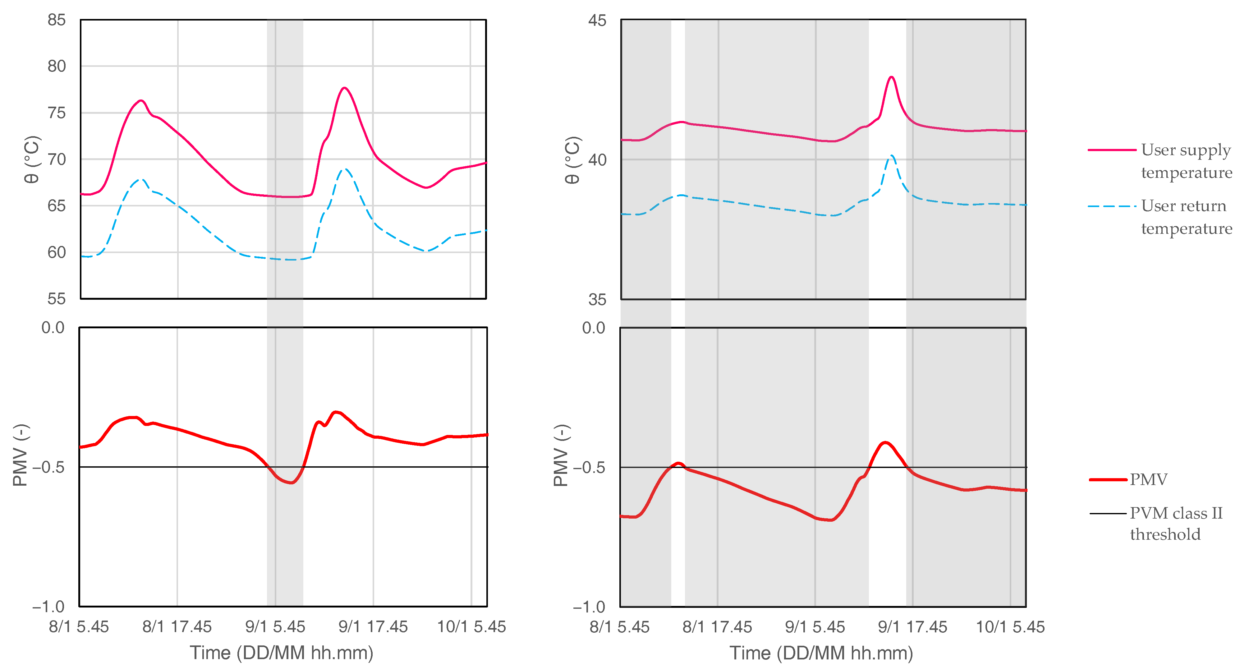
3.5. Comfort Indicators

The framework presented in Section 2.5 can be adopted to evaluate indoor comfort in buildings in the different retrofitting scenarios. In the choice of the evaluation method, it has been considered that adaptive concepts can be applied when the occupants have direct control on the surrounding environment and are aware of it, which might be a borderline assumption in large multi-family buildings. Some studies report that the use of adaptive methodologies for design purposes led to too-cold buildings, as pointed out by Halawa et al. [54]. Therefore, PMV/PPD method has been chosen over the adaptive approach in a conservative perspective, and the following indicators have been used:

• Operative temperature, defined according to EN ISO 52016-1:2017 as:

  $${\theta }_{\mathrm{op}}=\frac{{\theta }_{\mathrm{air}}+{\theta }_{\mathrm{mr}}}{2}$$

  (16)

  for a qualitative evaluation of the transient periods.
• Minimum PMV calculated in the reference period T:

  $${PMV}_{\min }=\underset{\forall \mathit{t}\in \mathit{T}}{min}\left\{PMV\left(t\right)\right\}.$$

  (17)
• Percentage of time steps in the reference period in which the PMV is below the minimum threshold for the selected IEQ class, ${PMV}_{\mathrm{IEQ},\mathrm{l}}$, which is a modified version of the “percentage of outside the range” parameter:

  $$POR=\frac{{\sum }_{\forall \mathit{t}\in \mathit{T}}\left(PMV\left(t\right)\le {PMV}_{\mathrm{IEQ},\mathrm{l}}\right)}{N_{\mathit{T}}}·100,$$

  (18)

  where $N_{\mathit{T}}$ is the total number of time steps in the reference period.

The indoor thermal comfort calculation module has also been written in MATLAB. The reference period is the heating season for Italian climate zone E [53] (15 October–15 April). IEQ class II has been selected. Input parameters have been fixed to $M=1.2$ met, corresponding to a standing/relaxed activity, $v_{\mathrm{air}}=0.1$ m/s, a reasonably low value expected with radiator-based heating, $I_{\mathrm{cl}}=1.0$ clo, corresponding to typical winter indoor clothing, and RH 50%.

4. Results and Discussion

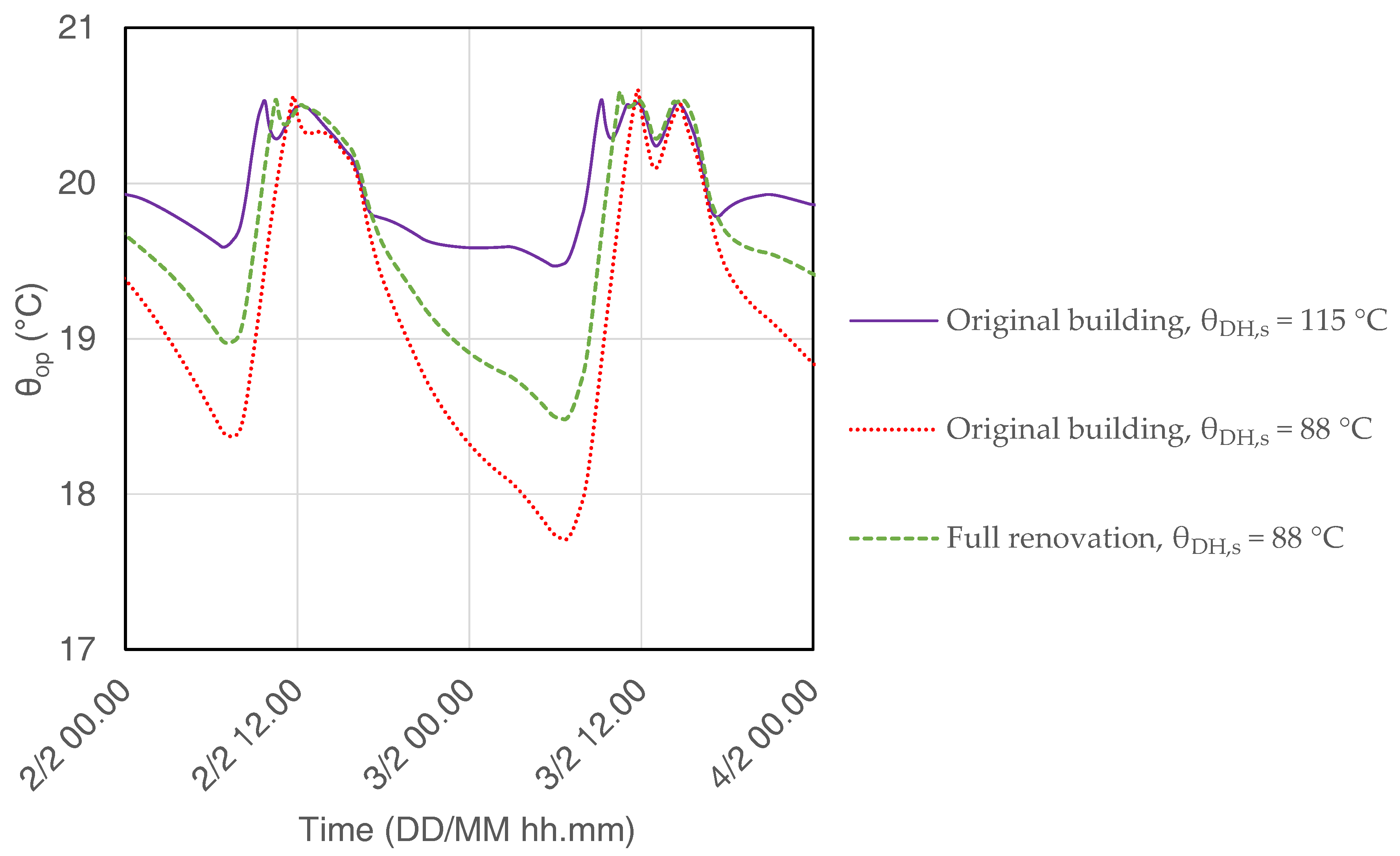
4.1. Baseline and Pre-Retrofitting

Hourly indoor air and mean radiant temperatures estimated by the energy calculation core are given as input to the thermal comfort module. The PMV for each time step is calculated with Equation (15), assuming the parameter values reported at the end of Section 3.5. Hourly PMVs are then used to obtain the desired aggregated indicators described in the same Section 3.5. This process is repeated for all the identified scenarios, namely:

• original building with design DH supply temperature;
• original building with reduced DH supply temperature;
• renovated building with reduced DH supply temperature,

where different DH temperature reduction levels and building renovation measures are explored. This process is performed for all the considered building types.

The modified POR parameter can be used to quantify the possible increase of discomfort occurrences when the DH temperature is decreased. It is expected that the lower the DH temperature with respect to the original (design) value, the higher the percentage of discomfort occurrences over the heating season. Figure 3 shows the variation of POR parameter with the reduction of DH supply temperature. Two decrease levels have been considered: ${\theta }_{\mathrm{DH},\mathrm{s}}$ = 115 ${}^{\circ }$C to ${\theta }_{\mathrm{DH},\mathrm{s}}$ = 95 ${}^{\circ }$C (representative of the shift from second to third generation DH) and ${\theta }_{\mathrm{DH},\mathrm{s}}$ = 115 ${}^{\circ }$C to ${\theta }_{\mathrm{DH},\mathrm{s}}$ = 88 ${}^{\circ }$C (which is slightly higher than the maximum user design supply temperature, set to 85 ${}^{\circ }$C for older buildings). It is worth noting that, since the POR associated to the original design conditions is zero, the $\mathsf{\Delta }POR$ represented in the bar charts numerically coincide with the POR of the reduced-temperature scenarios. As expected, the POR increases with decreasing DH supply temperature for all the building types. Although it rarely exceeds 5% in case of the smaller reduction (${\theta }_{\mathrm{DH},\mathrm{s}}$ = 95 ${}^{\circ }$C), the POR is non-negligible when the temperature is decreased to 88 ${}^{\circ }$C, especially for multifamily houses and recent buildings.

The latter result might look counter-intuitive. However, it can be explained in the light of the driving parameter for radiator heat transfer, that is, the LMTD between radiator and surrounding environment. Figure 4 shows an example of user supply and return temperatures obtained with ${\theta }_{\mathrm{DH},\mathrm{s}}=88$${}^{\circ }$C for a single-family house (SFH) built before 1900 and the same type of building built after 2006. It is worth reminding that the design user supply/return temperatures have been set as a function of the period of installation (see Table 2). In particular, they are 85/75 ${}^{\circ }$C and 60/40 ${}^{\circ }$C for the selected older building and newer building, respectively. It can be observed that the user flow/return temperatures following the reduction of DH supply temperature are still compatible with a decent radiator output in the older plant. On the other hand, in the recent building the decrease from design temperatures that are already low might quickly lead to insufficient heat outputs.

The above observation of the different role of the LMDT reduction in the two cases confirms that attention must be paid to low temperature systems (Figure 5). The nominal heat emission of a radiator scales with the ratio between actual and nominal LMTD, $\mathsf{\Delta }\theta /\mathsf{\Delta }{\theta }_{\mathrm{nom}}$, raised to the power of the radiator exponent, about 1.3. It can be seen how this ratio tends to be low for longer periods in case of low-temperature regime systems, as they are sized near the limit and, therefore, have little margin for further temperature reductions.

Since the percentage of time steps with too low PMV does not give any indication on the severity of the discomfort, the minimum value of PMV, $PM{V}_{\min }$, recorded during the heating season has also been taken into account. Figure 6, which refers to the case of ${\theta }_{\mathrm{DH},\mathrm{s}}=88$${}^{\circ }$C, shows indeed that lower PMV values are obtained on average for older buildings.

Further qualitative information about the severity of discomfort can be extracted from the analysis of the PPD distribution during the heating season. Figure 7 shows two examples of the evolution of PPD probability density distribution with decreasing DH supply temperatures for two single-family houses built in different periods. The mean PPD value does not change very much with the period of construction or with DH supply temperature, but the probability distribution does: the more recent building shows higher frequencies of low PPD (5–6%) for all DH supply temperatures, indicating a general higher degree of comfort. However, it also displays higher frequencies of high PPD (9–12%) when the temperature decreases from 115 ${}^{\circ }$C to 95 ${}^{\circ }$C and 88 ${}^{\circ }$C. On the other hand, very few occurrences of PPD below 6% can be observed in the older building irrespective of the DH supply temperature, but even after decreasing the latter to 95 ${}^{\circ }$C or 88 ${}^{\circ }$C the occurrence of PPD values above 10% remains relatively low.

Finally, dynamic calculations allow the direct observation of indoor transients, such as early morning warm-up. In Figure 8 a representative period is isolated in which the operative temperature in the design and in the reduced DH supply temperature conditions are compared for a single family house built in the period 1961–1975. It is expected that this effect be even magnified in case of intermittent control of the heating system (for example, on/off operation or set-back periods).

The results of the simulations show that, with the assumed design temperatures and interface heat exchangers, further actions are likely to be required not to affect the comfort of the occupants. A comparison between three possible scenarios is described in the next Subsection.

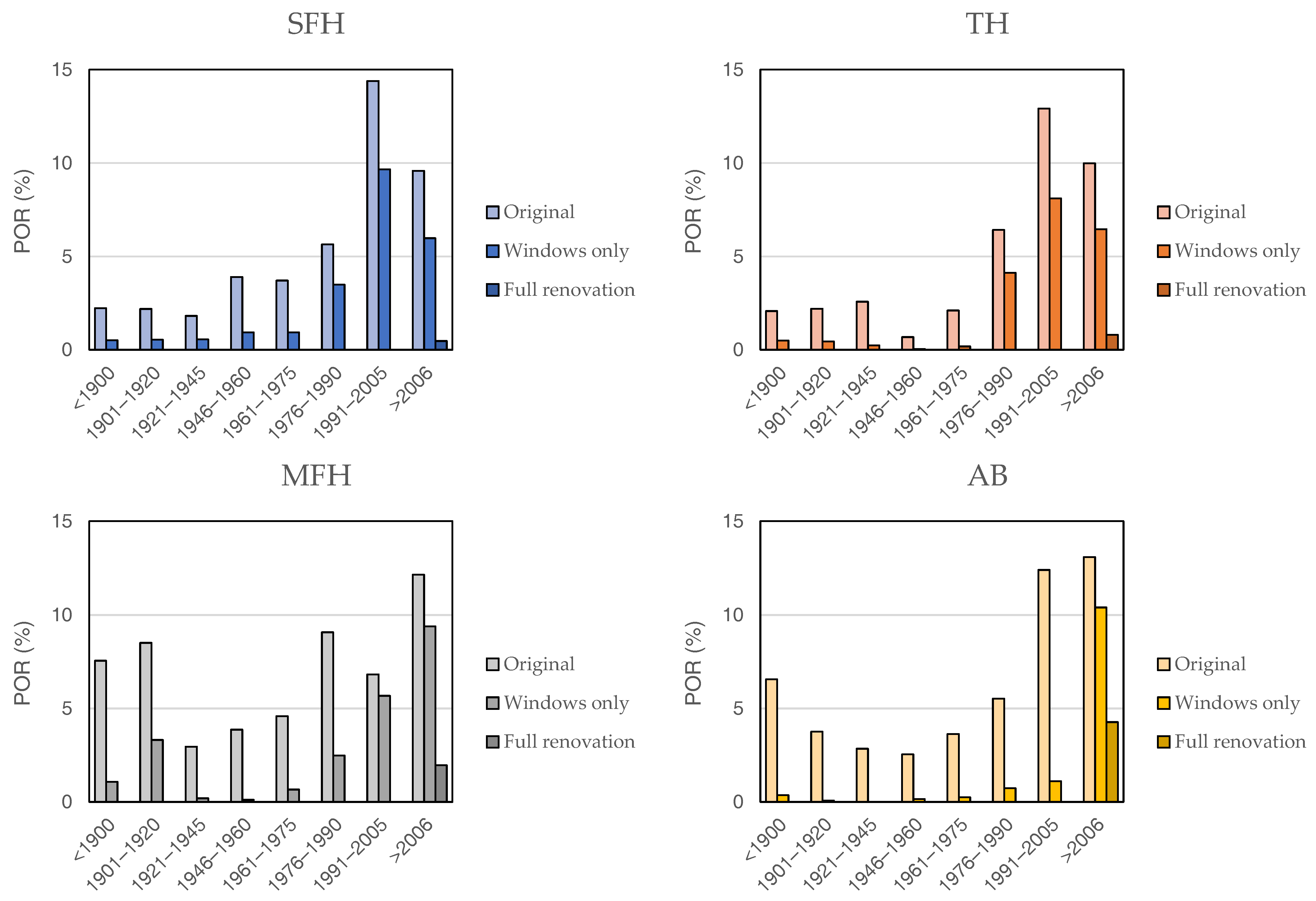
4.2. Three Retrofitting Scenarios

In the following, three possible sets of measures are compared. The first set consists of two actions on the primary (DH) side: heat exchanger replacement and flow rate increase. The new heat exchanger is sized so to provide twice the original thermal power, which is achieved with a larger number of plates and/or a higher heat exchange length (longer plates). For this set of simulations, the DH flow rate has not been capped to any value. Figure 9 shows the ratio between ${\dot{m}}_{\mathrm{DH}}$ and ${\dot{m}}_{\mathrm{DH},\mathrm{nom}}$, where ${\dot{m}}_{\mathrm{DH}}$ is the average DH flow rate that would be required to obtain the user supply temperature set-point with ${\theta }_{\mathrm{DH}}=88$${}^{\circ }$C and the oversized heat exchanger, and ${\dot{m}}_{\mathrm{DH},\mathrm{nom}}$ is the design flow rate in the initial state (${\theta }_{\mathrm{DH}}=115$${}^{\circ }$C and original heat exchanger). Once again, buildings built after the 1980s display a different behaviour than older buildings—in this case the effect of a lower design heating temperature regime is positive, in that the mere installation of a generously sized heat exchanger covers most of the new requirements. As expected, in older plants where the design conditions are close to the new DH supply temperature (85/75 ${}^{\circ }$C versus 88 ${}^{\circ }$C) the heat transfer on the heat exchanger is limited, and a larger increment of DH flow rate is required.

On the user side, two basic options are available—acting on the heating system or on the building fabric. Figure 10 shows the oversizing factor of the radiator, calculated as the ratio between the minimum LMTD recorded during the heating season with ${\theta }_{\mathrm{DH}}=88$${}^{\circ }$C and the original design LMTD, raised to the power of the radiator exponent, $k_{\mathrm{rad}}={({min}_{\forall \mathit{t}\in \mathit{T}}\left\{\mathsf{\Delta }{\theta }_{{88}^{\circ }\mathrm{C}}\left(t\right)\right\}/\mathsf{\Delta }{\theta }_{\mathrm{nom}})}^{{\mathit{n}}_{\mathrm{rad}}}$. The value looks quite stable for all the building types, irrespective of the construction period. According to this simulation, around 55% extra exchange area should be installed in private dwellings to fulfill the requirements, either by replacing existing radiators or by adding new ones. This measure is invasive and expensive, thus it does not appear to be the most indicated solution except maybe in public houses within the framework of a renovation campaign charged to the public owner.

The other obvious option is the partial or full renovation of the building fabric. Figure 11 shows the comparison of the POR parameters calculated with reduced DH supply temperature (${\theta }_{\mathrm{DH},\mathrm{s}}=88$ ${}^{\circ }$C) for all the building typologies in the following fabric conditions:

• Building in the original state
• Building with replaced windows
• Building with replaced windows and state-of-the-art insulation applied to the opaque elements

The reference for the retrofit measures is the “Usual” (or “Standard”) refurbishment set of measures described in the Italian TABULA/EPISCOPE deliverables [52] and defined on the basis of national and local regulatory framework [3]. It can be observed that the replacement of single-glass windows with high performance double-glazed windows greatly improves the comfort conditions in old buildings, especially in single family dwellings. For buildings built in the 1980s–1990s, improving the insulation of the opaque elements would be an effective solution. Conversely, none of these measures would be advisable for more recent buildings where the improvement margin is thin and the prospect of expensive works would face more resistance from the dwelling owners.

The renovation of poor energy performance buildings is clearly visible in the temperature transients: the improved insulation helps limiting the temperature decrease in the night-time and speeds up the reprise (Figure 12).

On an ending note, it is worth remarking that quantitative results depend on the heat exchanger models and the original design heating temperature regimes assumed for each building typology. If different hypotheses are made, for example, due to the availability of further information, the calculation may lead to different numerical values, although the key points of attention emerged from the present simulations are expected to be confirmed.

5. Conclusions

To evaluate the impact of district heating supply temperature reduction on the users, a comprehensive methodology has been presented that exploits the energy simulation results from a literature dynamic calculation method to assess indoor thermal comfort. The main innovative elements are the incorporation of an accurate model for the primary plate heat exchanger, and the use of comfort indicators to express the acceptability of district heating temperature reduction. Benefits of the proposed methodology are the limited input details to the energy calculation engine and a modular structure that allows for further expansions and tailoring.

The method has been applied to the case of existing buildings connected to a typical Northern Italian district heating network. The building stock has been represented by the TABULA/EPISCOPE Italian building typology matrix, in the conservative hypothesis of radiator-based heating systems. In the first set of simulations, the impact of decreasing district heating supply temperature has been analyzed. The results showed that key aspects to consider are the original sizing of the heating components and the original design conditions. As a consequence, the reduction of district heating supply temperature may result in longer periods of moderate discomfort in more recent buildings, and shorter periods of severe discomfort in older heating systems.

The second set of simulations different improvement scenarios have been evaluated. In particular, actions on the primary side appear to be suitable to more recent buildings, in which the fabric thermal performances are already fair to good, and the lower design heating temperature regime has a positive effect. For older buildings, improving opaque element insulation and/or replacing obsolete windows seems a wiser solution than installing additional heating power. Both strategies are indeed quantified as potentially invasive and expensive, but the former aims at reducing the energy needs and is therefore to be preferred.

The heating system model does not take into account distribution heat losses and original system oversizing, whose influence could be the subject of further studies. In this respect, the proposed methodology could also be applied to an actual urban area for which more detailed information is available, as well as measurements before and after the changing event. In the analysis of large buildings, the assumption of a single thermal zone for the whole building could be simplistic for the purpose of comfort assessment. A possible solution would be to simulate the behavior of the individual dwelling with the actual boundary conditions. This option is already included in the simulation framework. Future developments include the use of this method for studies related to district heating return temperature, heating control settings, and cost-benefit assessment on both the primary and the secondary heating side.

References

1. Abergel, T.; Delmastro, C. Tracking Buildings 2020. Available online: https://www.iea.org/reports/tracking-buildings-2020 (accessed on 18 October 2020).
2. Lowe, R. Technical options and strategies for decarbonizing UK housing. Build. Res. Inf. 2007, 35, 412–425. [Google Scholar] [CrossRef] [Green Version]
3. Ballarini, I.; Corgnati, S.P.; Corrado, V. Use of reference buildings to assess the energy saving potentials of the residential building stock: The experience of TABULA project. Energy Policy 2014, 68, 273–284. [Google Scholar] [CrossRef]
4. Di Turi, S.; Stefanizzi, P. Energy analysis and refurbishment proposals for public housing in the city of Bari, Italy. Energ. Policy 2015, 79, 58–71. [Google Scholar] [CrossRef]
5. Delmastro, C.; Mutani, G.; Schranz, L. The evaluation of buildings energy consumption and the optimization of district heating networks: A GIS-based model. Int. J. Energy Environ. Eng. 2016, 7, 343–351. [Google Scholar] [CrossRef] [Green Version]
6. Zirak, M.; Weiler, V.; Hein, M.; Eicker, U. Urban models enrichment for energy applications: Challenges in energy simulation using different data sources for building age information. Energy 2020, 190, 116292. [Google Scholar] [CrossRef]
7. Tronchin, L.; Fabbri, K. Energy Performance Certificate of building and confidence interval in assessment: An Italian case study. Energy Policy 2012, 48, 176–184. [Google Scholar] [CrossRef]
8. Nageler, P.; Zahrer, G.; Heimrath, R.; Mach, T.; Mauthner, F.; Leusbrock, I.; Schranzhofer, H.; Hochenauer, C. Novel validated method for GIS based automated dynamic urban building energy simulations. Energy 2017, 139, 142–154. [Google Scholar] [CrossRef]
9. Mutani, G.; Todeschi, V. Building energy modeling at neighborhood scale. Energy Effic. 2020, 13, 1353–1386. [Google Scholar] [CrossRef]
10. Torabi Moghadam, S.; Toniolo, J.; Mutani, G.; Lombardi, P. A GIS-statistical approach for assessing built environment energy use at urban scale. Sustain. Cities Soc. 2018, 37, 70–84. [Google Scholar] [CrossRef]
11. Tronchin, L.; Manfren, M.; James, P. Linking design and operation performance analysis through model calibration: Parametric assessment on a Passive House building. Energy 2018, 165, 26–40. [Google Scholar] [CrossRef] [Green Version]
12. Noussan, M.; Nastasi, B. Data Analysis of Heating Systems for Buildings—A Tool for Energy Planning, Policies and Systems Simulation. Energies 2018, 11, 233. [Google Scholar] [CrossRef] [Green Version]
13. Mancini, F.; Nastasi, B. Energy retrofitting effects on the energy flexibility of dwellings. Energies 2019, 12, 2788. [Google Scholar] [CrossRef] [Green Version]
14. Westermann, P.; Deb, C.; Schlueter, A.; Evins, R. Unsupervised learning of energy signatures to identify the heating system and building type using smart meter data. Appl. Energy 2020, 264, 114715. [Google Scholar] [CrossRef]
15. Tronchin, L.; Fabbri, K. Analysis of buildings’ energy consumption by means of exergy method. Int. J. Exergy 2008, 5, 605–625. [Google Scholar] [CrossRef]
16. Kaarup Olsen, P.; Christiansen, C.H.; Hofmeister, M.; Svendsen, S.; Thorsen, J.E. Guidelines for Low-Temperature District Heating; Technical report; Danish Energy Agency and EUDP 2010-II. 2014. Available online: https://www.danskfjernvarme.dk/-/media/danskfjernvarme/gronenergi/projekter/eudp-lavtemperatur-fjv/guidelines-for-ltdh-final_rev1.pdf (accessed on 10 November 2020).
17. Sameti, M.; Haghighat, F. Optimization of 4th generation distributed district heating system: Design and planning of combined heat and power. Renew. Energ. 2019, 130, 371–387. [Google Scholar] [CrossRef]
18. Neri, M.; Luscietti, D.; Pilotelli, M. Computing the Exergy of Solar Radiation From Real Radiation Data. J. Energy Resour.-ASME 2017, 139, 061201. [Google Scholar] [CrossRef] [Green Version]
19. Piana, E.A.; Grassi, B.; Socal, L. A Standard-Based Method to Simulate the Behavior of Thermal Solar Systems with a Stratified Storage Tank. Energies 2020, 13, 266. [Google Scholar] [CrossRef] [Green Version]
20. Nuytten, T.; Claessens, B.; Paredis, K.; Van Bael, J.; Six, D. Flexibility of a combined heat and power system with thermal energy storage for district heating. Appl. Energy 2013, 104, 583–591. [Google Scholar] [CrossRef]
21. Iora, P.; Beretta, G.P.; Ghoniem, A.F. Exergy loss based allocation method for hybrid renewable-fossil power plants applied to an integrated solar combined cycle. Energy 2019, 173, 893–901. [Google Scholar] [CrossRef]
22. Lund, H.; Østergaard, P.A.; Chang, M.; Werner, S.; Svendsen, S.; Sorknæs, P.; Thorsen, J.E.; Hvelplund, F.; Mortensen, B.O.G.; Mathiesen, B.V.; et al. The status of 4th generation district heating: Research and results. Energy 2018, 164, 147–159. [Google Scholar] [CrossRef]
23. Buffa, S.; Cozzini, M.; D’Antoni, M.; Baratieri, M.; Fedrizzi, R. 5th generation district heating and cooling systems: A review of existing cases in Europe. Renew. Sustain. Energy Rev. 2019, 104, 504–522. [Google Scholar] [CrossRef]
24. Østergaard, D.; Svendsen, S. Are typical radiators over-dimensioned? An analysis of radiator dimensions in 1645 Danish houses. Energy Build. 2018, 178, 206–215. [Google Scholar] [CrossRef]
25. Tunzi, M.; Østergaard, D.S.; Svendsen, S.; Boukhanouf, R.; Cooper, E. Method to investigate and plan the application of low temperature district heating to existing hydraulic radiator systems in existing buildings. Energy 2016, 113, 413–421. [Google Scholar] [CrossRef]
26. Østergaard, D.; Svendsen, S. Theoretical overview of heating power and necessary heating supply temperatures in typical Danish single-family houses from the 1900s. Energy Build. 2016, 126, 375–383. [Google Scholar] [CrossRef] [Green Version]
27. Wang, Q.; Ploskić, A.; Holmberg, S. Retrofitting with low-temperature heating to achieve energy-demand savings and thermal comfort. Energy Build. 2015, 109, 217–229. [Google Scholar] [CrossRef]
28. Bo, M. Riqualificazione dei vecchi impianti di riscaldamento a radiatori. Aicarr J. 2012, 12, 20–28. [Google Scholar]
29. Millar, M.A.; Burnside, N.; Yu, Z. An investigation into the limitations of low temperature district heating on traditional tenement buildings in Scotland. Energies 2019, 12, 2603. [Google Scholar] [CrossRef] [Green Version]
30. Ashfaq, A.; Ianakiev, A. Investigation of hydraulic imbalance for converting existing boiler based buildings to low temperature district heating. Energy 2018, 160, 200–212. [Google Scholar] [CrossRef] [Green Version]
31. Neirotti, F.; Noussan, M.; Riverso, S.; Manganini, G. Analysis of Different Strategies for Lowering the Operation Temperature in Existing District Heating Networks. Energies 2019, 12, 321. [Google Scholar] [CrossRef] [Green Version]
32. Crabb, J.A.; Murdoch, N.; Penman, J.M. A simplified thermal response model. Build. Serv. Eng. Res. Technol. 1987, 8, 13–19. [Google Scholar] [CrossRef]
33. Michalak, P. The simple hourly method of EN ISO 13790 standard in Matlab/Simulink: A comparative study for the climatic conditions of Poland. Energy 2014, 75, 568–578. [Google Scholar] [CrossRef]
34. CEN/TC 89. EN ISO 52016-1:2017 Energy Performance of Buildings— Energy Needs for Heating and Cooling, Internal Temperatures and Sensible and Latent Heat Loads—Part 1: Calculation Procedures; European Committee for Standardization, CEN: Brussels, Belgium, 2017. [Google Scholar]
35. Mazzarella, L.; Scoccia, R.; Colombo, P.; Motta, M. Improvement to EN ISO 52016-1:2017 hourly heat transfer through a wall assessment: The Italian National Annex. Energy Build. 2020, 210, 109758. [Google Scholar] [CrossRef]
36. Campana, J.P.; Morini, G.L. BESTEST and EN ISO 52016 Benchmarking of ALMABuild, a New Open-Source Simulink Tool for Dynamic Energy Modelling of Buildings. Energies 2019, 12, 2938. [Google Scholar] [CrossRef] [Green Version]
37. Lundström, L.; Akander, J.; Zambrano, J. Development of a space heating model suitable for the automated model generation of existing multifamily buildings—A case study in Nordic climate. Energies 2019, 12, 485. [Google Scholar] [CrossRef] [Green Version]
38. Déqué, F.; Ollivier, F.; Poblador, A. Grey boxes used to represent buildings with a minimum number of geometric and thermal parameters. Energy Build. 2000, 31, 29–35. [Google Scholar] [CrossRef]
39. Yu, W.; Li, B.; Jia, H.; Zhang, M.; Wang, D. Application of multi-objective genetic algorithm to optimize energy efficiency and thermal comfort in building design. Energy Build. 2015, 88, 135–143. [Google Scholar] [CrossRef]
40. Manfren, M.; Nastasi, B.; Groppi, D.; Astiaso Garcia, D. Open data and energy analytics-An analysis of essential information for energy system planning, design and operation. Energy 2020, 213, 118803. [Google Scholar] [CrossRef]
41. Tronchin, L.; Manfren, M.; Nastasi, B. Energy efficiency, demand side management and energy storage technologies—A critical analysis of possible paths of integration in the built environment. Renew. Sustain. Energy Rev. 2018, 95, 341–353. [Google Scholar] [CrossRef]
42. Braulio-Gonzalo, M.; Bovea, M.D.; Ruá, M.J.; Juan, P. A methodology for predicting the energy performance and indoor thermal comfort of residential stocks on the neighbourhood and city scales. A case study in Spain. J. Clean. Prod. 2016, 139, 646–665. [Google Scholar] [CrossRef] [Green Version]
43. Carlucci, S.; Pagliano, L.; Sangalli, A. Statistical analysis of the ranking capability of long-term thermal discomfort indices and their adoption in optimization processes to support building design. Build. Environ. 2014, 75, 114–131. [Google Scholar] [CrossRef]
44. Stasi, R.; Liuzzi, S.; Paterno, S.; Ruggiero, F.; Stefanizzi, P.; Stragapede, A. Combining bioclimatic strategies with efficient HVAC plants to reach nearly-zero energy building goals in Mediterranean climate. Sustain. Cities Soc. 2020, 63, 102479. [Google Scholar] [CrossRef]
45. Ballarini, I.; Costantino, A.; Fabrizio, E.; Corrado, V. The Dynamic Model of EN ISO 52016-1 for the Energy Assessment of Buildings Compared to Simplified and Detailed Simulation Methods. Build. Simul. 2019, 2019, 3847–3854. [Google Scholar] [CrossRef]
46. Teskeredzic, A.; Blazevic, R. Transient Radiator Room Heating—Mathematical Model and Solution Algorithm. Buildings 2018, 8, 163. [Google Scholar] [CrossRef] [Green Version]
47. Wang, L.; Sunden, B.; Manglik, R.M. Plate Heat Exchangers: Design, Applications and Performance, 2nd ed.; Wit Pr/Computational Mechanics: Southampton, UK; Boston, MA, USA, 2007. [Google Scholar]
48. Longo, G.A.; Righetti, G.; Zilio, C.; Ortombina, L.; Zigliotto, M.; Brown, J.S. Application of an Artificial Neural Network (ANN) for predicting low-GWP refrigerant condensation heat transfer inside herringbone-type Brazed Plate Heat Exchangers (BPHE). Int. J. Heat Mass Transf. 2020, 156, 119824. [Google Scholar] [CrossRef]
49. Wright, A.; Heggs, P. Rating Calculation for Plate Heat Exchanger Effectiveness and Pressure Drop Using Existing Performance Data. Chem. Eng. Res. Des. 2002, 80, 309–312. [Google Scholar] [CrossRef]
50. Associazione Italiana Riscaldamento Urbano, AIRU. Il Riscaldamento Urbano-Annuario 2019; Editrice Alkes: Milan, Italy, 2019. [Google Scholar]
51. Ballarini, I.; Corrado, V. A New Methodology for Assessing the Energy Consumption of Building Stocks. Energies 2017, 10, 22. [Google Scholar] [CrossRef] [Green Version]
52. Politecnico di Torino, Energy Department. Joint EPISCOPE and TABULA Website—Italy Country Page. Available online: https://episcope.eu/building-typology/country/it/ (accessed on 14 May 2020).
53. D.P.R. 26/08/1993, n. 412—Regolamento Recante Norme per la Progettazione, L’installazione, L’esercizio e la Manutenzione Degli Impianti Termici Degli Edifici ai Fini del Contenimento dei Consumi di Energia, in Attuazione Dell’art. 4, Comma 4, Della Legge 9 Gennaio 1991, n. 10. 1993. Available online: https://www.gazzettaufficiale.it/eli/id/1993/10/14/093G0451/sg (accessed on 30 July 2020). (In Italian).
54. Halawa, E.; van Hoof, J. The adaptive approach to thermal comfort: A critical overview. Energy Build. 2012, 51, 101–110. [Google Scholar] [CrossRef]
Figure 1. Modular calculation framework.
Energies 14 00025 g001
Figure 2. Schematic representation the heating system within the general model.
Energies 14 00025 g002
Figure 3. Variation of percentage outside range (POR) parameter with decreased district heating (DH) temperature (115 C to 95 C and 115 C to 88 C).
Energies 14 00025 g003
Figure 4. Top: user supply/return temperatures in a winter period in a single family house built before 1900 (left) and a single family house built after 2006 (right) after decreasing the DH temperature from 115 C to 88 C. Bottom: corresponding PMVs. Discomfort periods are indicated by the gray areas.
Energies 14 00025 g004
Figure 5. Ratio between actual and design LMTD for an old single family house built before 1900 (solid line) and a new single family house built after 2006 (dashed line), for the same period of the year as in Figure 4. Discomfort periods are indicated by the hatched area (old building) and the gray area (new building).
Energies 14 00025 g005
Figure 6. Minimum predicted mean vote (PMV) recorded in the heating season for the different types of buildings as a function of construction period. Gray area: standard deviation of the PMVs for the different building types.
Energies 14 00025 g006
Figure 7. Distribution of predicted percentage of dissatisfied (PPD) over the heating season for single family house built between 1961–1975 (left) and built after 2006 (right), and decreasing DH supply temperatures.
Energies 14 00025 g007
Figure 8. Indoor operative temperature in a winter period for a single family house built between 1961 and 1975 at different DH supply temperatures. Original design temperature: θ DH = 115 C. Operative temperature set-point: 20.5 C.
Energies 14 00025 g008
Figure 9. Ratio between the secondary flow rate need with decreased DH temperature ( θ DH = 88 C) and the original design flow rate ( θ DH = 115 C) for the different types of buildings as a function of construction period.
Energies 14 00025 g009
Figure 10. Radiator oversizing factor, k rad , for the different types of buildings as a function of construction period.
Energies 14 00025 g010
Figure 11. Variation of POR parameter with decreased DH temperature (115 C to 88 C) for different retrofit measures on the buildings: original building with no renovation (lightest shade); building with original opaque elements and state-of-the-art windows (intermediate shade); fully renovated building (darkest shade).
Energies 14 00025 g011
Figure 12. Indoor operative temperature in a winter period for a single family house built between 1961 and 1975. Operative temperature set-point: 20.5 C.
Energies 14 00025 g012