Abstract
Today, Formula 1 race cars are equipped with complex hybrid electric powertrains that display significant cross-couplings between the internal combustion engine and the electrical energy recovery system. Given that a large number of these phenomena are strongly engine-speed dependent, not only the energy management but also the gearshift strategy significantly influence the achievable lap time for a given fuel and battery budget. Therefore, in this paper we propose a detailed low-level mathematical model of the Formula 1 powertrain suited for numerical optimization, and solve the time-optimal control problem in a computationally efficient way. First, we describe the powertrain dynamics by means of first principle modeling approaches and neural network techniques, with a strong focus on the low-level actuation of the internal combustion engine and its coupling with the energy recovery system. Next, we relax the integer decision variable related to the gearbox by applying outer convexification and solve the resulting optimization problem. Our results show that the energy consumption budgets not only influence the fuel mass flow and electric boosting operation, but also the gearshift strategy and the low-level engine operation, e.g., the intake manifold pressure evolution, the air-to-fuel ratio or the turbine waste-gate position.
1. Introduction
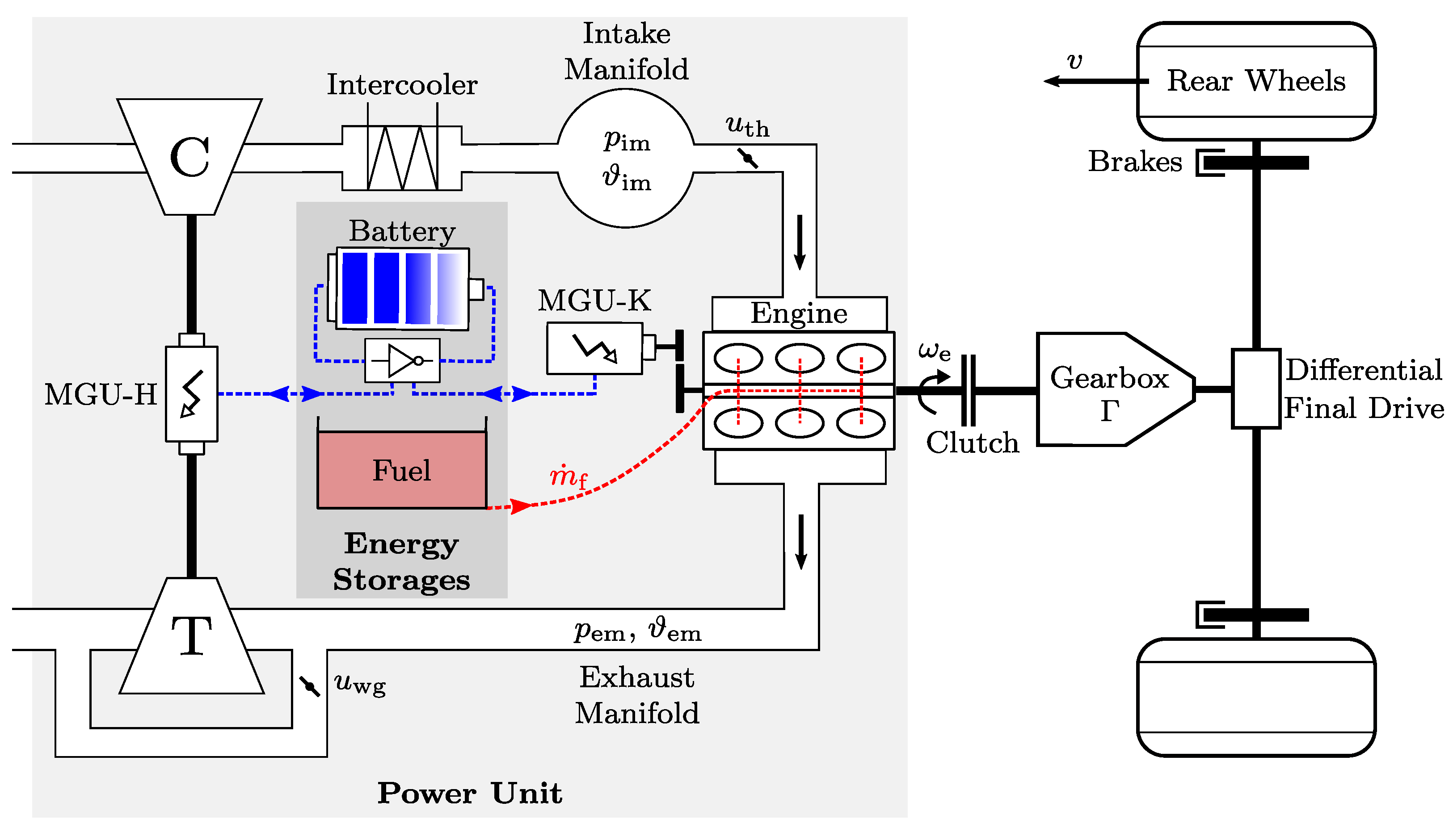
Formula 1 (F1) is the top category for single-seater circuit racing and features the fastest racing cars in the world. In the past, these were powered by V8, V10 or even V12 engines. Since 2014, however, the Fédération Internationale de l’Automobile (FIA) [1,2] has prescribed the parallel hybrid powertrain topology shown in Figure 1. In this so-called power unit, the main source of propulsive power is still the internal combustion engine, but in the form of a downsized and turbocharged V6 with a displacement volume of . However, the engine is supplemented by an electric recovery system composed of two electric motor generator units, denoted by motor generator units (MGUs), and an electric energy storage in the form of a battery. The MGU-K (K for kinetic) is coupled to the engine’s crankshaft and is used to increase the propulsive power of the car or to recuperate energy during braking. To increase the powertrain’s efficiency, the FIA allows the installation of a second electric motor on the turbocharger shaft, referred to as MGU-H (H for heat). As a consequence, the turbine is oversized and in general produces more power than absorbed by the compressor, such that part of the energy contained in the hot exhaust gases can be recuperated by the MGU-H and fed to the battery or directly to the MGU-K. Additionally, the MGU-H can be used to speed up the compressor to avoid turbo lag. While the FIA restricts the MGU-K power to , no limits are imposed on the MGU-H. Finally, the power unit is connected to the wheels by an eight-speed sequential gearbox and a differential. In addition to the finite capacity of the battery of , the FIA also limits the fuel consumption for an entire race (≈300 km) to and constrains the maximum fuel mass flow as a function of the engine speed. Every F1 driver’s goal is to win the race, i.e., to complete the defined number of laps in the shortest amount of time. Therefore, controlling the powertrain in a time optimal way is of utmost importance. The complex interactions between the thermal and the electrical part, which are coupled not only through the drivetrain but also through the electrified turbocharger, together with the limited available energy imposed by the FIA rules, call for a rigorous model-based optimization of the powertrain operation. Since the behavior of several internal combustion engine components highly depends on the engine speed, any offline optimization must also take into account the gearshift strategy. Therefore, in this paper we present a framework that jointly computes the time-optimal control and gearshift strategy for a detailed low-level model of the current hybrid electric F1 powertrain. In the following paragraphs, we review the relevant literature, formulate the research statement and outline our contribution, and give an overview on the paper structure.
Figure 1.
Schematic representation of the main components of the Formula 1 (F1) hybrid electric powertrain.
Given that the F1 power unit is hybrid electric, the methodology applied to optimize its energy management can be related to hybrid electric vehicle research: for road-going vehicles, such as passenger cars, the main objective is to minimize the fuel consumption, whilst for race cars the key performance indicator is the lap time. Therefore, we identify two streams of research related to our topic. The first one deals with the fuel-optimal control of hybrid electric vehicles, where in the majority of the cases the power request and the vehicle speed are known and given, i.e., the vehicle is assumed to follow a specific driving cycle. Non-causal optimal control strategies were investigated using dynamic programming [3,4,5], convex optimization [6,7,8] and Pontryagin’s minimum principle [9,10,11]. The sizing of the powertrain components [12], of the drivetrain [13,14] or the design of the powertrain topology [15] were also discussed in previous works. For feedback control, equivalent consumption minimization strategies have been applied for fuel consumption minimization [16,17] considering also pollutant emissions [18], the battery state of health [19] or turbocompounding [20,21]. Furthermore, the integer nature of gears and the engine on/off choice were tackled with iterative algorithms [7], Pontryagin’s minimum principle [22,23], dynamic programming [8,23], outer convexification [24,25,26,27,28] and shooting or bisection methods [29,30]. However, all these approaches mainly rely on quasi-static system models and ignore the dynamic behavior of the internal combustion engine, e.g., the intake manifold or the turbocharger dynamics. To properly capture the engine dynamics, mean value engine models are usually formulated using nonlinear differential equations [31,32,33,34] and optimized offline [35,36,37,38,39,40] or online in a model predictive control fashion [41,42,43,44]. Recently, the air path of a forced-intake engine was modeled in a quasi-static manner as a basis for minimum fuel control [45,46]. However, in these works several assumptions about the air-to-fuel ratio and the turbocharger operation were made to render the resulting model convex. In Ref. [47] instead, a piecewise affine low-level model of a high-performance hybrid electric power unit is presented. The proposed model includes the most relevant low-level engine dynamics, as well as the integer nature of the cylinder deactivation, and presents a methodology to fit the highly nonlinear turbocharger maps by means of neural networks techniques. While the resulting fuel-optimal mixed integer linear program has global optimality guarantees, it relies on measured engine speed and power request trajectories, i.e., the gearshift command and the vehicle speed are not optimized but are given. The second stream of research concerns the time-optimal control of race cars. In Ref. [48,49,50], the authors solved the general problem of evaluating the vehicle lateral and longitudinal control that yields to the minimum time maneuvering around a racetrack. Structural components that additionally influence the achievable lap time were included in the optimization framework: the suspensions [51] and the tyres [52]. The computation of the optimal driving trajectory was further extended with the inclusion of power flows [53], of the F1 specific power flows and regulations [54], or of the power flows and therewith associated thermal management of a Formula E race car [55]. Finally, the authors of [56] show that the time-optimal energy management marginally influences the race car’s velocity evolution in the corners, whilst it significantly impacts its speed on the straights. The most important assumption made in the previous works on F1 in our group, is to decouple the energy management from the driving path: we assume the driver to be responsible for following the time-optimal path on the racetrack, whilst we put the focus on the optimal usage of the available energy [57,58,59,60,61,62]. The time-optimal control strategies for race and qualifying scenarios were solved numerically in [57,60], while real-time feedforward and feedback control architectures were derived analytically and tested in [58,59]. A two-level model predictive control architecture was also proposed as an online controller in [62] and afterwards extended with adaptation algorithms in [61]. Finally, in [63] we combined convex optimization, dynamic programming and Pontryagin’s minimum principle in an iterative scheme to solve the energy management and gearshift control of a modern F1 powertrain. However, the majority of the models used for minimum time optimization are high-level models that mainly rely on quasi-static formulations, ensuring low computational times in the order of seconds to minutes. Thus, they can serve a rapid parametrization of the energy management but neglect important effects such as transient motor generator unit (MGU)-H operation during the gearshifts. Moreover, they do not consider the dynamics of the engine, e.g., the intake manifold and the turbocharger, they do not model the engine cylinder deactivation and do not include the air-to-fuel ratio and the spark advance influence on the achievable engine power.
To the best of the authors’ knowledge, there exists no framework so far that jointly computes the time-optimal control and gearshift strategy for a detailed low-level model of a F1 hybrid electric powertrain. The impact of both the gearshift strategy and the targets for fuel and battery usage on the engine power generation and on the low-level dynamics, e.g., on the air-to-fuel ratio or on the intake manifold pressure evolution, has not been studied yet for time-optimal control purposes. Therefore, in this paper we propose a detailed low-level mathematical formulation of the F1 powertrain suited for numerical optimization. Beside the specific focus on the engine speed dependency of each powertrain’s component, we propose a continuous nonlinear model to describe the engine cylinder deactivation and reformulate non-smooth inequality constraints such that they can be accommodated by off-the-shelf nonlinear solvers. We relax the resulting mixed integer nonlinear model using outer convexification techniques, thereby reducing computational times for solving the time-optimal control problem by two orders of magnitude. The presented framework can be used as a tool to benchmark the low-level actuation of the internal combustion engine components in the context of the time-optimal energy management. Specifically, the suboptimality of the control strategy adopted during a race week-end can be assessed, reference trajectories for online control can be generated and control heuristics can be inferred. Moreover, the framework allows to perform parametric studies aimed at the design of new powertrain components. For the purpose of this work, only a part of the FIA sporting and technical regulations [1,2] are considered and modeled. As an example, specific limits on the energy transfer between the battery and the electric motor connected to the crankshaft are not implemented. This is due to confidentiality reasons and also facilitates the results analysis given the complexity of the system.
The paper is structured as follows: in Section 2 we present a mixed integer nonlinear model of the F1 hybrid electric powertrain and the car’s longitudinal dynamics, especially focusing on the engine speed dependency, the dynamic behavior of the intake manifold and the turbocharger, as well as the engine cylinder deactivation. Thereafter, we formulate the time-optimal control problem and apply outer convexification. In Section 4 we present parameter studies where we compute and discuss the time-optimal control strategies for different energy budgets and operational limits, both over portions of lap and entire lap. Finally, conclusions are drawn in Section 5.
2. Modeling of the Formula 1 Powertrain
In this section we identify and validate a detailed low-level model of the F1 hybrid electric powertrain. A schematic of the system is shown in Figure 1 and its mathematical mean-value model formulation suited for numerical optimization is mostly based on or inspired by [31,47,57].
In addition to the energy storages onboard, i.e., the battery and the fuel tank, the power unit consists of an internal combustion engine equipped with an electrified turbocharger and two motor generator units: the MGU-K is mounted on the engine shaft and is used for electric boosting or regenerative braking, whilst the MGU-H is an electric motor that converts part of the heat contained in the hot exhaust gases into electrical energy or reduces the turbo lag. The engine system is composed of an intake manifold equipped with an intercooler and a throttle valve, a 1.6 L gasoline direct injection engine with cylinder deactivation capabilities, an exhaust manifold and a turbocharger. The turbocharger consists of a radial compressor, a radial turbine equipped with a waste-gate valve and the MGU-H mounted on the turbocharger shaft. Finally, the remaining part of the powertrain consists of a gearbox and a differential that connect the engine and the MGU-K to the wheels.
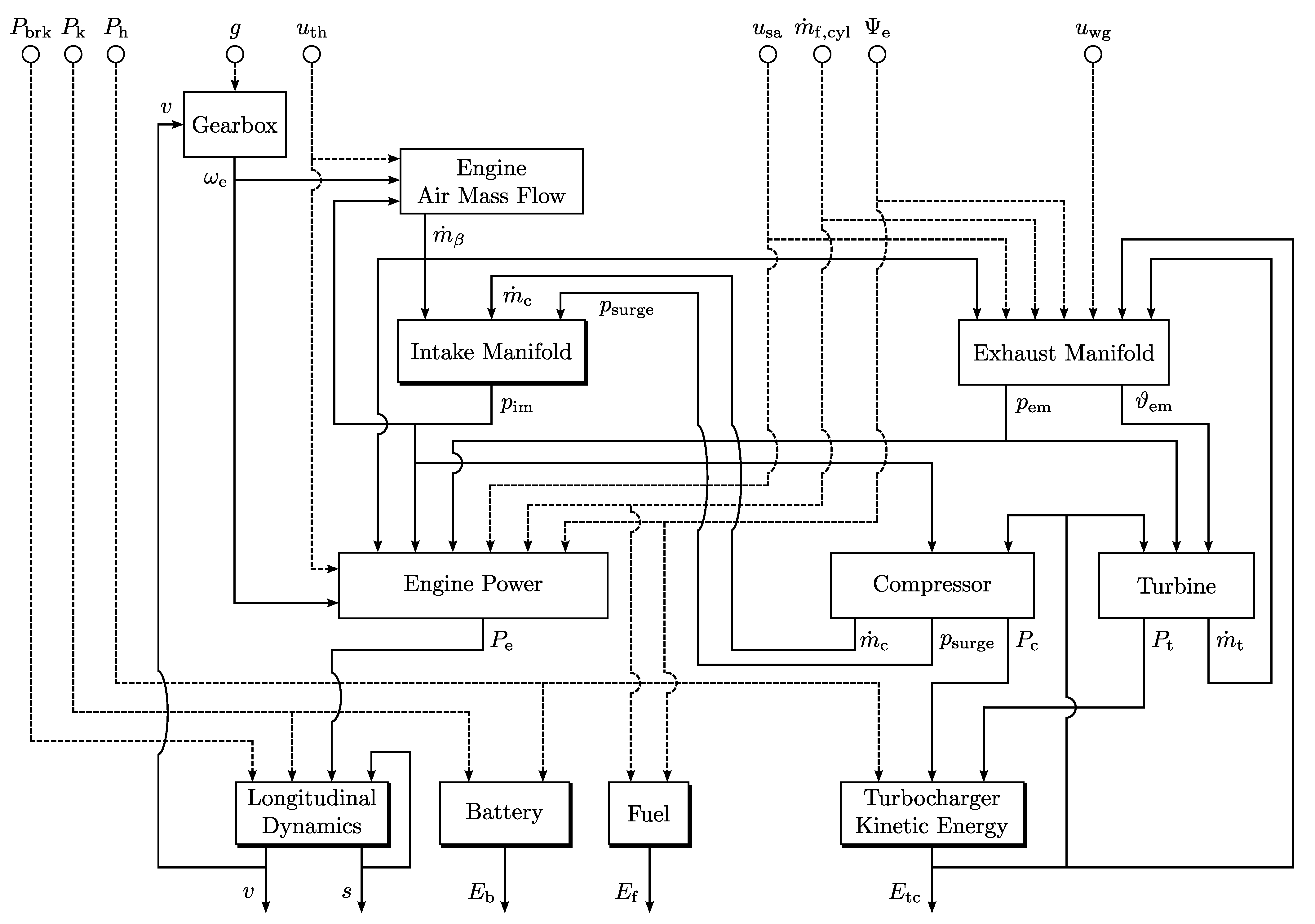
A schematic representation of how the state and the input variables of the considered system relate to each other, is displayed in the causality diagram shown in Figure 2. The system’s state variables are the car’s velocity v and its position s on the racetrack, the intake manifold pressure , the turbocharger rotational kinetic energy , the battery energy and fuel energy consumed. In contrast to the intake manifold dynamic behavior, the exhaust manifold is modeled as a static subsystem. This modeling assumption will be motivated in Section 2.4. The system’s input variables are the power of the friction brakes , the MGU-K power , the MGU-H power , the engaged gear g, the throttle valve position , the spark-advance position , the cylinder fuel mass flow , the cylinder deactivation variable and the waste-gate valve position . The powertrain model is partly taken or inspired by the works conducted at our institute or published by ourselves. Specifically, the energy recovery system model in Section 2.5 and the longitudinal dynamics in Section 2.6 are taken from [57]. The linear waste-gate model in Section 2.3 and the static approximation of the exhaust manifold in Section 2.4 are taken from our previous work [47], where the engine speed over the entire mission was given and we made use of integer variables and linear equations to model a high-performance power unit. For confidentiality reasons, the model parameters cannot be disclosed and the data shown on the plots are normalized and denoted by . For instance, the normalized value of the turbine mass flow is denoted by . To quantify the modeling mismatch, we use the normalized mean absolute error defined as
where N is the number of data points considered, is the modeled value and is the measured one. The data displayed in the Figures 3, 5–10 are telemetry data acquired during a race week-end on a current F1 hybrid electric race car by our industrial partner. For confidentiality reasons, we are not allowed to disclose the exact experimental setup used to obtain them, i.e., sensor specification and placement. The majority of the data are acquired directly by means of sensors, e.g., intake manifold pressure, or are computed online by means of maps that were recorded on dedicated test-benches, e.g., compressor and turbine mass flow maps. Finally, all the validation plots shown in the following sections cover roughly a third of the racetrack and include three straights and two corners.
Figure 2.
Causality diagram of the system. The shaded blocks represent the dynamical subsystems, the plain blocks the static/algebraic subsystems and the dashed lines the control inputs of the system.
2.1. Intake Manifold
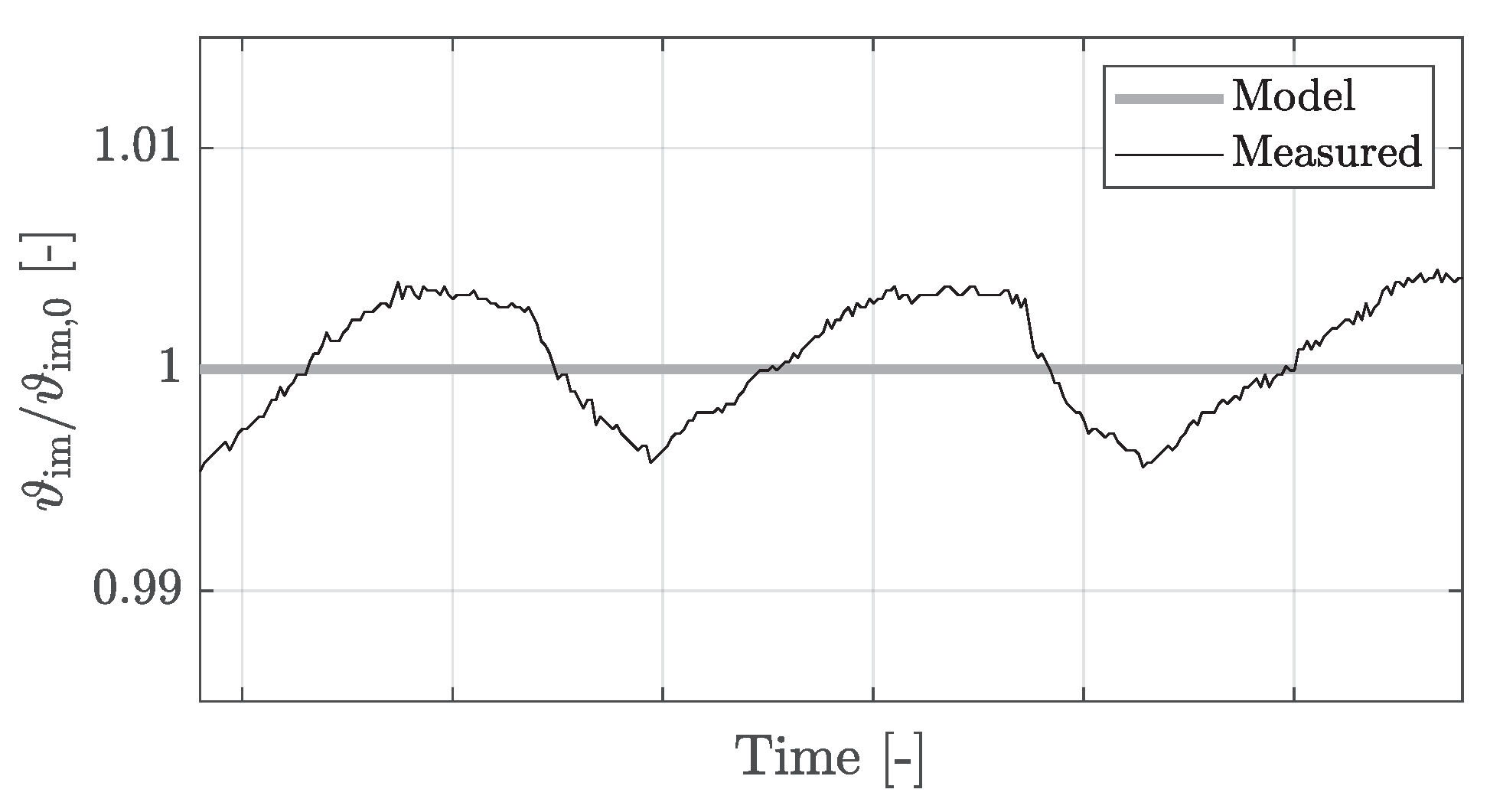
The intake manifold is modeled as an isothermal receiver [31], since the intercooler operation leads to temperature fluctuations over one lap of less than , as Figure 3 shows. As a consequence, we assume a constant temperature inside the intake manifold.
Figure 3.
Measured and modeled intake manifold temperature ().
We then model the dynamics of the intake manifold pressure as
where is the intake manifold volume, is the specific gas constant of air, is the compressor mass flow and is the engine air mass flow. The engine air mass flow is modeled as
where is the engine speed, is the engine displacement volume, is the volumetric efficiency and is the throttle position. Since the throttle is placed after the plenum, the intake manifold pressure dependency [31] of the volumetric efficiency is neglected. The map that relates the volumetric efficiency to the engine speed is identified using the neural network technique presented in Appendix C. For confidentiality reasons, it cannot be displayed.
2.2. Engine Power and Cylinder Deactivation
The internal combustion engine power is the sum of three contributions: the engine power stemming from the fuel combustion , the engine power losses due to the pistons’ friction and the engine pumping power arising from the gas exchange in the intake and exhaust manifold. Therefore we model the engine power as
Since the engine features cylinder deactivation, the engine combustion power is the sum of all the cylinder-individual combustion power values:
where denotes the engine combustion power delivered by cylinder . It is defined as
where is the fuel lower heating value and is the amount of fuel injected in cylinder i. The combustion efficiency is engine speed dependent, whereas and are cylinder individual correction factors that capture the influence of the air-to-fuel ratio and spark-advance position, respectively. Since all cylinders share the same engine speed and, if active, we assume the same amount of fuel injected , air-to-fuel ratio and spark-advance, (6) can be rewritten as
where the cylinder deactivation variable defines the number of active cylinders. This variable is assumed to be continuous to reduce the calculation complexity (more on that in Section 3.2). The total fuel mass flow injected is therefore
while the change in fuel energy consumption is modeled as
The maximum amount of fuel injected per cylinder is limited by the FIA regulations [1,2]:
where the speed-dependent maximum allowed fuel injection in is
where is the engine speed threshold imposed by the FIA regulations. To implement this non-smooth constraint in the optimization framework, we rewrite and relax (11) and introduce the lifting variable in the following manner:
Finally, using (12) we can rewrite (10) as
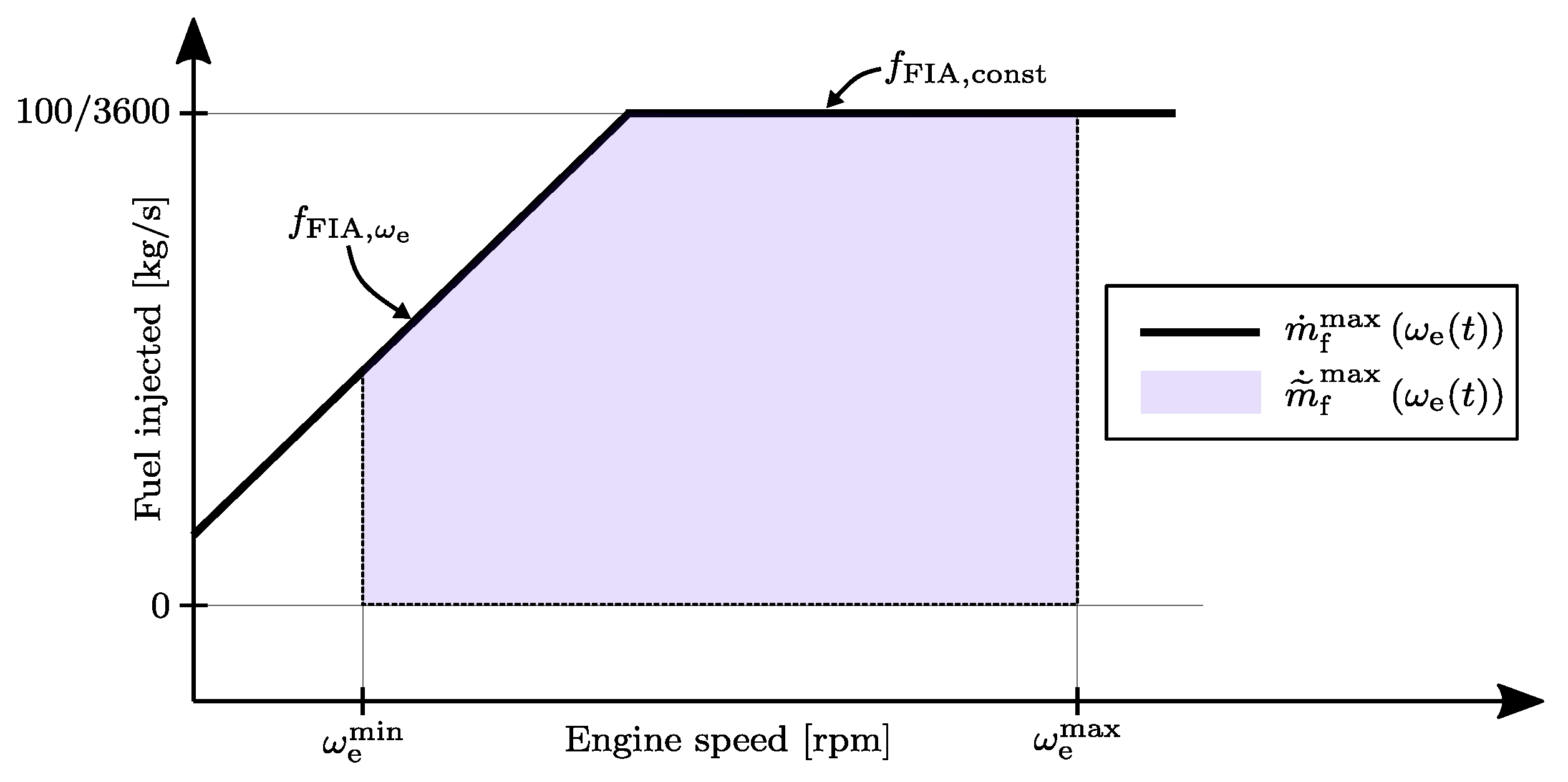
The reformulation (12) is schematically drawn in Figure 4 and can be interpreted as follows: if the engine speed is below the maximum amount of fuel that can be injected is constrained by the engine-speed dependent ramp ; if the engine speed is above , the maximum amount of fuel is limited by the constant constraint .
Figure 4.
Fédération Internationale de l’Automobile (FIA) regulation on the maximal allowed fuel mass flow [1,2].
The spark-advance efficiency depends on the spark advance position and the engine speed . The relationship is usually defined by a map . We assume that for any engine speed we can realize a spark-advance efficiency and in post-processing compute the spark-advance position which realizes the desired efficiency. The engine speed efficiency is modeled as
where , and are coefficients subject to identification. Next, we introduce the definition of the air-to-fuel ratio in the cylinder [31]
where is the stoichiometric constant. The main drawback of (15) is its singularity if no fuel is injected, i.e., for . For this reason, we introduce the fuel-to-air ratio , which is defined as
The fuel-to-air ratio is always defined and bounded, since the engine air mass flow cannot be zero during operation. Furthermore, the fuel-to-air ratio mixture has an impact on the combustion efficiency, which is defined by the map . Similar to the engine speed efficiency maps, the fuel-to-air ratio efficiency maps usually present a peak efficiency at the optimal fuel-to-air ratio value and gradually decrease in an asymmetric way if the fuel-to-air ratio is larger or smaller than that [31]. To properly capture the asymmetric form of the map, the fuel-to-air ratio efficiency is fitted using the neural network techniques presented in Appendix C. If a cylinder is activated, i.e., , the fuel-to-air ratio must lie in the allowed range [31], leading to the case distinction
It is worth noticing that can be any value if . Ideally, when the engine is completely shut off, i.e., , the fuel-to-air ratio should be zero because no fuel should be injected, i.e.,
Since it is computationally expensive to implement (18), we neglect it for the following reason: If , the fuel injected in the cylinders is constrained by both the FIA regulations (11) and the fuel-to-air ratio constraints (17); If , the fuel injected in the cylinders is only constrained by the FIA regulations, but it will not have an impact on any algebraic or dynamic equation of the model, e.g., on the combustion engine power in (7) or the fuel energy dynamics in (9), since is always multiplied with . Finally, we make use of so-called vanishing constraints [64] to rewrite (17) as
The engine friction power is modeled as a quadratic function of the engine speed as
where , and are coefficients subject to identification. Finally, the engine pumping power is modeled as
where is the exhaust manifold pressure and is a coefficient subject to identification. Figure 5 shows the fitting of the engine combustion, friction and pumping power. Whilst all three power contributions match precisely the measurements data on the straights, the friction and pumping powers partially differ during the corners, i.e., where the engine is not operated at full load. Regarding the friction power, this might be attributable to the simple model which lacks additional (input or state) dependencies, whilst the difference in the pumping power might be due to physical phenomena that zero-dimensional models are not able to capture properly.
Figure 5.
Measured and modeled engine combustion power (), friction power () and pumping power ().
2.3. Turbocharger and Waste-Gate
The turbocharger’s state variable is its rotational kinetic energy defined as
where is the moment of inertia of the entire turbocharger and is the rotational speed of the shaft. The rotational kinetic energy evolves as a function of the turbine power , compressor power and MGU-H power acting on the shaft:
In Ref. [47], it was shown that the compressor and turbine mass flows and powers can be accurately described as a function of the turbocharger rotational energy , the intake manifold pressure , the exhaust manifold pressure and exhaust manifold temperature . Therefore, these quantities can be represented with the following multi-dimensional maps :
This is a direct consequence of the assumption that the pressure and temperature at the compressor entrance, as well as the pressure after the turbine, are assumed to be constant and equal to the ambient conditions [47].
Both compressor and turbine are subject to operational limits. While the mechanical, blocking and choke limits of the compressor can be accounted for by introducing constant constraints on the turbocharger rotational speed and compressor mass flow, the compressor surge limit varies depending on the turbocharger rotational speed:
In order to avoid compressor operation in the surge region, we introduce the constraint
All the turbocharger maps are fitted using the neural network modeling technique presented in Appendix C. Since the turbine and the waste-gate mass flows are well approximated as orifices [31] and share the same exhaust manifold pressure and temperature, the waste-gate mass flow is modeled as [47]
where is the normalized waste-gate position and is defined as
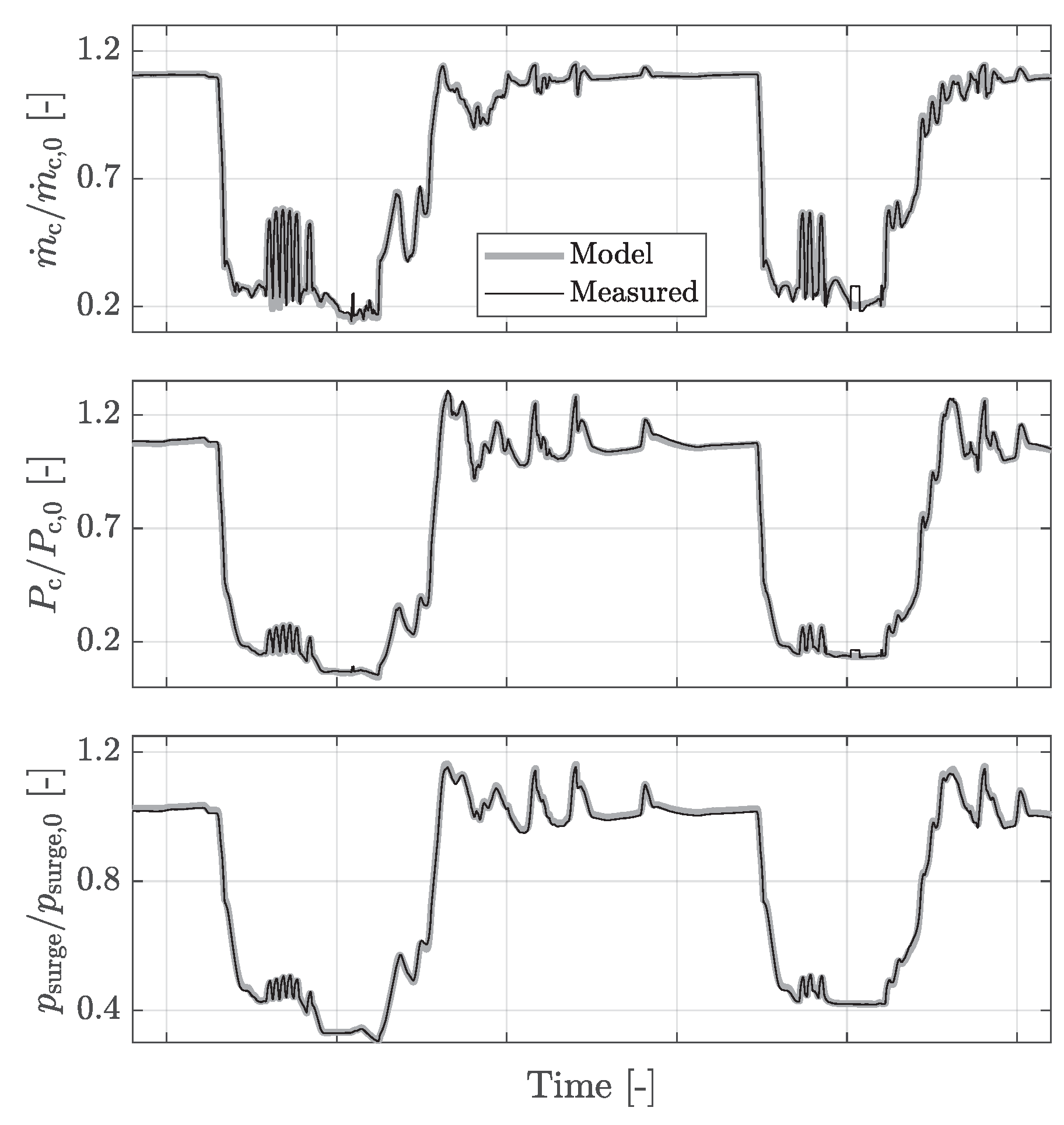
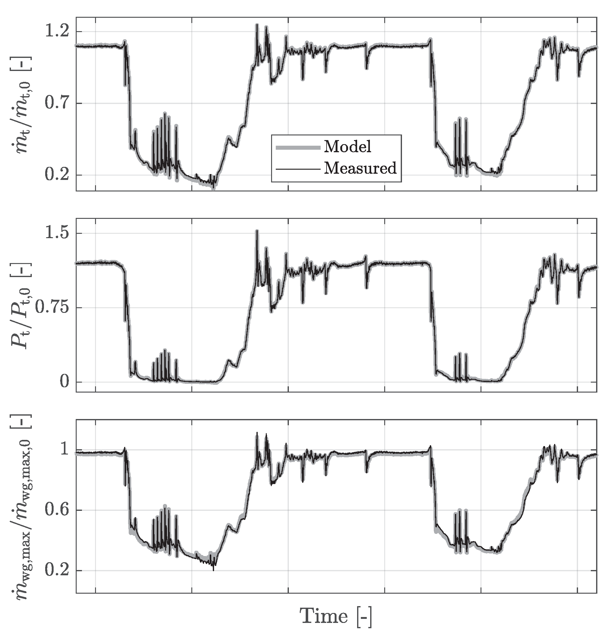
with and being parameters subject to identification. Figure 6 and Figure 7 show that the fitting precision of the turbocharger quantities and the waste-gate maximum mass flow is satisfactory, with very good agreement between the model and the measurements.
Figure 6.
Measured and modeled compressor mass flow (), compressor power () and compressor surge ().
Figure 7.
Measured and modeled turbine mass flow (), turbine power () and maximum waste-gate mass flow ().
2.4. Exhaust Manifold
The exhaust manifold of the considered engine displays a small gas residence time and its volume is much smaller compared to the one of the intake manifold. As a consequence, we approximate the exhaust manifold to be quasi-static and adiabatic [31]. In Ref. [47], this simplification was shown to satisfactorily approximate the dynamic nature of a small plenum. Therefore, the exhaust manifold temperature is modeled as an algebraic function
where is the temperature of the gases exiting cylinder i. Since we assume all the active cylinders to share the same combustion conditions, and the inactive cylinders to share the same non-combustion conditions, (32) can be rewritten as
where the variables and represent the engine-out temperature if the cylinder is active and inactive, respectively. The engine-out temperature of the active cylinders is modeled by superposing an enthalpic balance and a temperature increase induced by the spark-advance retardation [65,66,67]
with
where is the temperature of the injected fuel, is the heat capacity at constant pressure of the exhaust gases and is a fitting coefficient that represents how much combustion enthalpy goes into the exhaust manifold in form of heat. The term accounting for the temperature increase due to the ignition delay is
where is a fitting coefficient that represents how much the exhaust manifold temperature is increased by the extra heat arising from the spark-advance retardation.
Finally, the engine-out temperature of an inactive cylinder is modeled as in [47] by
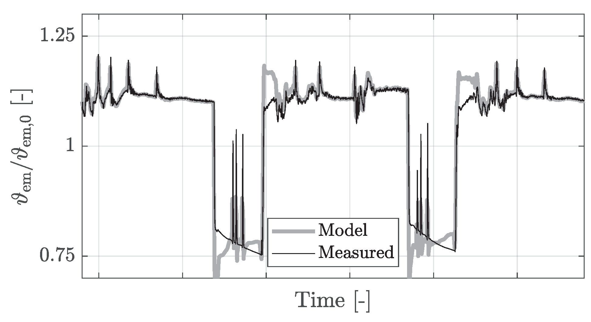
where and are coefficients subject to identification. The model (37) captures that the engine-out temperature is colder for a higher engine air-mass flow. Figure 8 shows the comparison of the exhaust manifold temperature model to measurement data. The proposed model properly captures the behavior on the straights where the temperature is high, especially during the upshifts (recognizable as little peaks), whereas it overestimates the temperature in the last part of the corner. This might be attributable to the quasi-static modeling choice, which entails the absence of the receiver’s inertia.
Figure 8.
Measured and modeled exhaust manifold temperature ().
Following the quasi-static modeling approach, the pressure in the exhaust manifold is implicitly defined through the algebraic mass balance
In Section 2.3, it was shown that the waste-gate mass flow can be approximated as a function of the turbine mass flow and the waste-gate position , i.e.,
and that the turbine mass flow is a function of the turbocharger rotational kinetic energy , exhaust manifold pressure and exhaust manifold temperature , i.e.,
If we combine (38) with (39), we obtain
Finally, combining (41) with (40) the exhaust manifold pressure is found to be
The exhaust manifold pressure map is identified using the neural network technique presented in Appendix C and its fitting is shown in Figure 9. Despite its quasi-static modeling, the exhaust manifold pressure partially displays a dynamic behavior: this is due to its dependency on the engine air mass flow, which is a function of two dynamic variables, i.e., the intake manifold pressure and the car’s velocity.
Figure 9.
Measured and modeled exhaust manifold pressure ().
2.5. Energy Recovery System
In this section, we model the energy recovery system using a high-level modeling approach [57]. The power conversion losses of the motor generator units (MGUs) from mechanical-to-electrical conversion and vice-versa are approximated using the quadratic functions
where and are the electrical powers of the MGUs, and the mechanical power of the MGUs, and and coefficients subject to identification. The MGUs electrical actuator limits are considered, namely
The battery electrical losses can also be approximated using a quadratic model
where is the internal battery power, is the terminal battery power, a coefficient subject to identification and a constant auxiliary power.
Figure 10 shows the satisfactory fitting precision of the MGU-H, MGU-K and battery power conversions. Finally, we assume a constant battery voltage [68,69] and model the battery energy dynamics as an open integrator [47,57], i.e.,
Figure 10.
Measured and modeled MGU-K electrical power (), MGU-H electrical power () and battery internal power ().
2.6. Longitudinal Dynamics and Gearbox
In this section we present the longitudinal dynamics and the gearbox of the race car. The position s of the car on the circuit evolves according to its velocity v, hence
The lateral dynamics of the car are condensed [57] into a track-dependent maximum velocity profile which constrains the velocity at each position of the racetrack
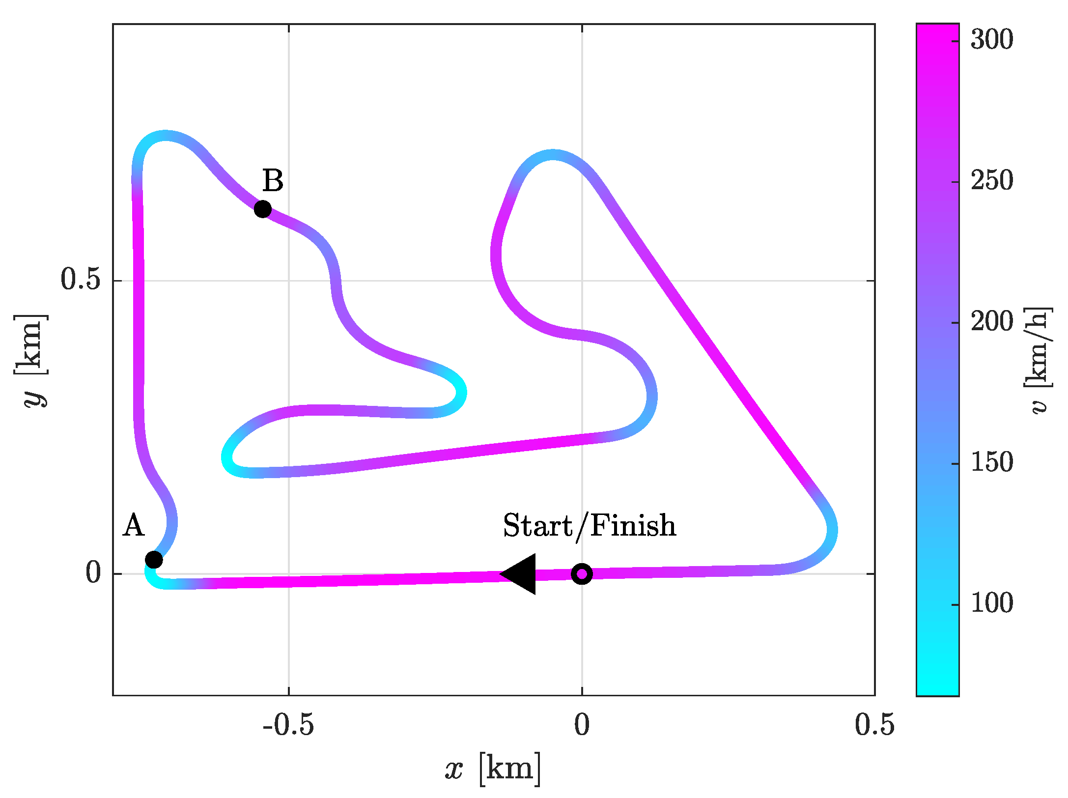
The achievable velocity when the driver is not fully pressing the accelerator pedal, i.e., in the corners, is inferred from the telemetry data or using sophisticated simulations of the car’s lateral dynamics, while the maximum velocity constraint on the straight is set constant and equal to a value that is not achievable, e.g., . As an example, in Figure 11 we depict a measurement of the car’s velocity on the layout of the Bahrain International Circuit.
Figure 11.
Track layout of the Bahrain International Circuit with a color-coded representation of the F1 car velocity measured during a race week-end. This specific racetrack layout is used in Section 4 for the results and case studies. The points A and B mark the beginning and end of the track segment investigated in Section 4.
The longitudinal dynamics are modeled as [57]
with
where is the car mass, , , and are the aerodynamic, curvature, drag reduction (DRS) and rolling coefficient subject to identification, is a position-dependent curvature parameter that accounts for the aerodynamic change during cornering of open wheeled cars, is a position-dependent boolean (where in DRS zones, otherwise 0), G is the gravitational acceleration and is the traction power. The traction power is defined as
where is the power dissipated in the friction brakes and is the propulsive power modeled as [57]
where and are the slip coefficients subject to identification and is the total power unit power, i.e., . More details on the longitudinal model and its validation can be found in [57]. Finally, the power unit is equipped with an eight-speed gearbox, i.e., . The overall transmission of the gear g from the engine shaft to the car’s wheel is denoted by . Therefore the engine speed whit the gear engaged is related to the velocity by
and the engine speed is constrained for drivability and regulatory reasons [1,2] as
3. Optimal Control Problem
In this section, we state the optimal control problem. The state variables are the position s, the car’s velocity v, the intake manifold pressure , the turbocharger’s rotational kinetic energy , the battery energy and the fuel energy . The input variables are the throttle position , the waste-gate position , the cylinder fuel mass flow , the cylinder deactivation variable , the spark-advance efficiency , the MGU-K power , the MGU-H power , the braking power and the engaged gear g.
3.1. Objective and Space Domain
The objective of the optimal control problem is to minimize the lap time
subject to the system dynamics and constraints presented in Section 2, as well as the energy consumption targets imposed on the fuel and on the battery as terminal constraints:
As presented in Section 2.6, the track-dependent parameters, e.g., the maximum velocity profile or the track curvature , are given as a function of the position on the track. Therefore, we reformulate the optimal control problem in space domain with the following change of variable based on (47)
where and are the differential variables in space and in time domain, respectively. While the algebraic equations and constraints do not change, the differential equations change as follows:
where is the right-hand side of the differential equation in time domain and is its counterpart in space domain. Finally, the objective function changes to
where T is the time necessary to cover the considered track length S.
3.2. Outer Convexification and Rounding
The model presented in Section 2 contains an integer variable, i.e., the engaged gear. Since mixed-integer optimization is computationally expensive [70], we convexify the model with respect to the integer variables using the outer convexification methodology [71,72,73]. Specifically, we introduce a control variable for each gear choice , with the bijection
Furthermore, we impose the variables to fulfill the special ordered set type 1 property (SOS-1), i.e.,
Next, we relax the problem by making the integer variable continuous , i.e.,
The outer convexified differential equations of the system read as
while the inequality constraints of the form
read as
The detailed formulation of the outer convexified optimal control problem is presented in Appendix A. Finally, to construct an integer sequence of the gear command from the relaxed optimal one , a rounding strategy is applied. Due to the conditions imposed by the equality constraint in (61), the rounding strategy should not violate the SOS-1 property. Therefore, we use the rounding methodology proposed in [74] that reads as
where is an auxiliary variable of gear g at point i introduced to make (67) more readable, is the distance between two space points and i is the space point at which the rounding is sought. This recursive methodology simultaneously takes into account all gears up to and favors the choice of the smallest gear g with the largest .
Regarding the engine cylinder deactivation, the variable is treated as continuous, although it is integer by nature. This is done to reduce the calculation time and complexity, i.e., to avoid introducing relaxed integers at each time step instead of only. In addition to that, the solution to this problem can be used as a benchmark to compare the results obtained with an integer number of active cylinders and assess the resulting suboptimality. Finally, for the sake of completeness, we compare in Appendix B the relaxed and rounded nonlinear solution to the original mixed-integer nonlinear program solution. The results highlight that the trajectories of the two solutions are close to identical and that the lap time difference is negligible, thereby justifying the outer convexification approach.
3.3. Numerical Solution Method
We discretize the optimization problem using the multiple shooting method and the standard explicit Euler integration method, which approximates the continuous derivative of the variable as
where is the space domain discretization length, is the discrete space variable, is the number of discrete steps and S is the considered track length. The optimization problem is implemented in MATLAB [75] using the symbolic framework CasADi [76] and solved with IPOPT [77]. Furthermore, the mixed-integer nonlinear program (MINLP) solution presented in Appendix B is computed using BONMIN with the branch-and-bound algorithm [78]. In [47], it was shown and validated that sampling frequencies larger than were able to properly capture the intake manifold and turbocharger dynamics. Since the optimization problem is described in space domain, we pre-compute a variable space domain discretization length for a specific (time domain) sampling frequency using a nominal car’s velocity trajectory measured during a race week-end on a particular circuit:
While it is most likely that the optimized velocity profile will not be the same as the nominal one in each point of the track, the sampling frequency does not deviate more than 0.9–1.2 Hz on average for entire lap optimizations. The computational time to solve both the relaxed and the rounded nonlinear program solutions on a desktop computer varies from minutes to hours and depends on the chosen boundary conditions and the space horizon length. As an example, if only a small portion of the lap is considered, e.g., a straight with two corners, the computational time is between 5 and 20 min. If the entire lap is considered, the computational time varies between 2 and 4 h. Finally, the MINLP displays computational times up to 100 times slower compared to the presented methodology.
4. Results
In this section, we show the results of the time-optimal control problem presented in Section 3 for racing scenarios on the Bahrain International Circuit, a lap of which takes roughly . The racetrack under consideration influences the vehicle dynamics through its specific maximum velocity profile, path curvature and DRS zones. Our non-causal optimization framework is not based on a driving cycle, since the velocity profile and the propulsive power are subject to optimization. First, we analyze over a portion of the lap the optimal gearshift and power unit control from a low-level point of view. Second, we extend the analysis to entire lap results.
4.1. Detailed Analysis on a Portion of the Lap
In this subsection we present several case studies where we apply the proposed optimization framework to practically relevant strategy and design decisions. To facilitate a detailed analysis, we consider only a portion of the lap. We start by comparing the optimal control of the power unit for two different battery recharge targets, which is a strategy parameter that can be changed by the driver during a race. Thereafter, we add a constraint on the compressor outlet temperature to showcase how the presented framework can support the design choice of the intercooler dimension.
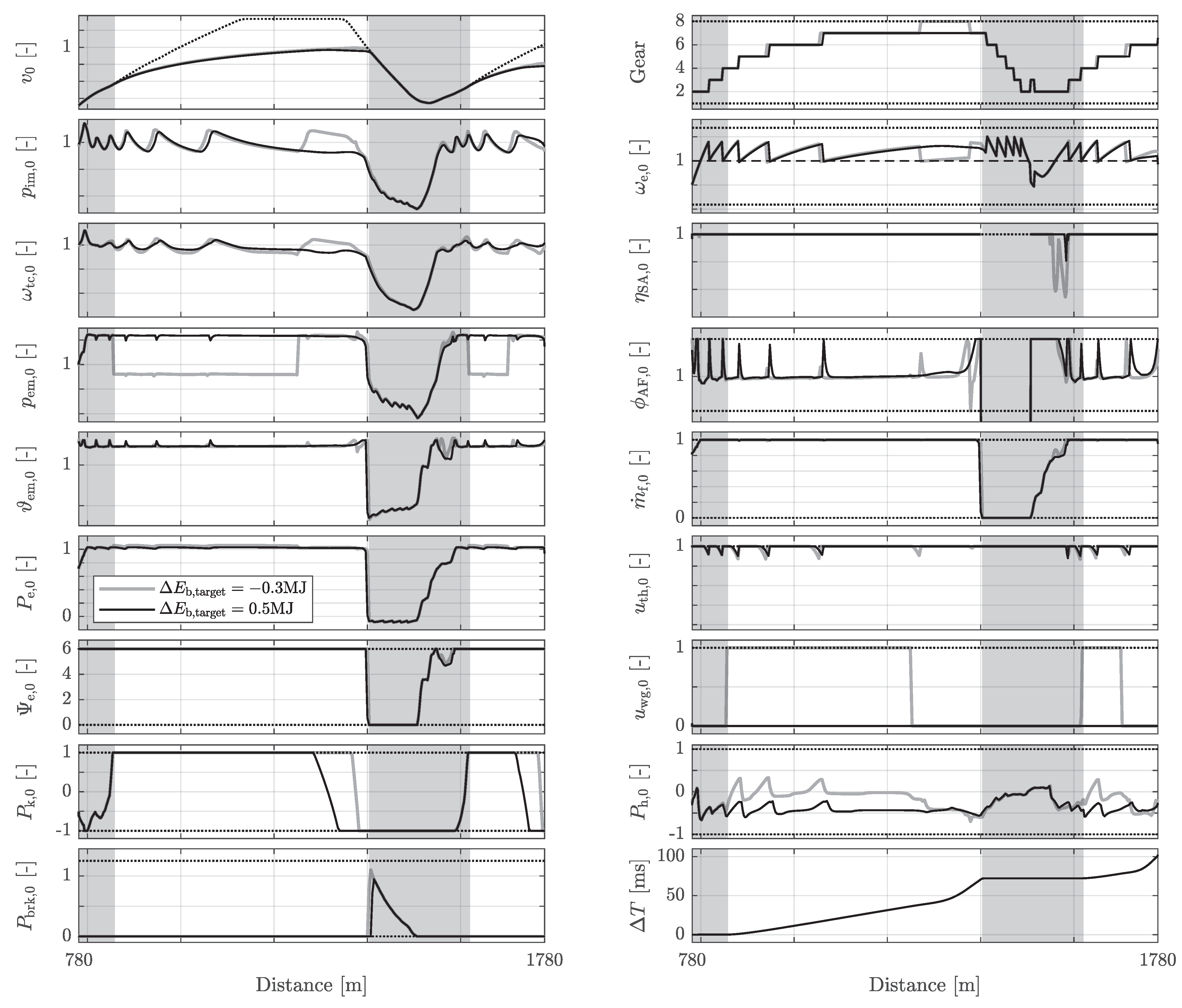
Figure 12 shows the most significant optimal state and input trajectories for two different battery recharge targets and the same fuel consumption target. The considered portion of lap is the section between the points A and B in Figure 11. It can be noticed that the gearshift strategy is different: not only is the 8th gear solely engaged for the battery discharge case (), but also several upshifts occur earlier compared to the battery recharge case (). This trend can be attributed to the abundance of electrical energy at disposal: the gears are selected to maximize the overall engine power and therefore the propulsive power. For the battery recharge case, however, the trade-off between the engine power and the MGU-H recuperation is more pronounced. The fact of not shifting into the 8th gear keeps the engine speed high and therefore the pressure in the intake manifold lower (compared to the battery discharge case). As a consequence, the compressor power is lower and more power can be recuperated by the MGU-H. The power unit control around the upshifts occurs each time in a similar manner: the MGU-H recuperates less to accelerate the turbocharger shaft, whilst the throttle valve is operated to achieve the optimal fuel-to-air ratio value. The battery recharge target also influences the waste-gate operation. In conventional gasoline turbocharged engines, the waste-gate is operated to diminish the turbine power and thereby controls the intake manifold pressure [79]. By contrast, for the considered high-performance power unit the waste-gate is used to increase the engine power by diminishing the exhaust manifold pressure. The turbine power extraction is reduced and therefore the MGU-H power recuperation goes roughly to zero (when no upshift is taking place). The intake manifold pressure is not affected, the engine pumping power increases and so does the overall engine power. In addition to that, the MGU-K operation is also influenced by the battery availability. Not only the MGU-K cut occurs later on the straight if more battery energy can be deployed, but also the slope is different: the analytical explanation for this can be found in [58]. Finally, the optimal behavior in the corner is analyzed. The optimal cylinder deactivation is mainly the same, except at the corner exit. In this region, for the battery discharge case, slightly more fuel is injected. At the same time the spark-advance is slightly retarded and produces a lower spark-advance efficiency. This causes a small increase in the exhaust manifold temperature and pressure, allowing the MGU-H to recuperate more. The procedure of converting a small portion of fuel energy into electrical energy through the increase of the exhaust manifold temperature is possible in the cases where the battery recharge targets allow it. For the battery recharge case, this operation only occurs for a very short amount of time, since every drop of fuel counts and the gearshift strategy is not aimed at maximizing the engine efficiency, but rather finding the optimal trade-off between the internal combustion engine and the energy recovery system.
Figure 12.
Optimal state and input trajectories over a portion of the lap for two different battery recharge targets and the same fuel consumption target. The grey areas represent the regions where the constraint on the car’s velocity is active. The dotted lines are the state and input constraints, whilst the dashed line in the engine speed plot is placed at .
Next, we investigate the suboptimality entailed by a smaller intercooler choice in Figure 13. In such a case, to keep the same intake manifold temperature, the compressor outlet temperature needs to be lowered. As an example we include a constraint to decrease the maximum outlet temperature of the compressor by compared to the unconstrained case, i.e., . The compressor outlet temperature was modeled using the assumptions presented in Section 2.3 and fitted with the methodology of Appendix C, i.e., . To better visualize the transient phenomena during the gearshifts, thin vertical lines have been inserted at the upshift locations. The battery recharge target and fuel consumption target are the same for both scenarios. It can be noticed at first glance that the intake manifold and turbocharger speed trajectories are different and almost everywhere lower compared to the unconstrained case. This is mainly due to their dependency on the compressor outlet temperature. In addition, the engine air and fuel mass flows, as well as the gearshift strategy, differ markedly to case studies previously analyzed. Since the intake manifold pressure is (indirectly) limited, the gearshifts occur at higher engine speeds to avoid large engine air mass flow deficits after the upshift. Despite the throttle valve being completely opened after the upshifts, the fuel mass flow is limited by the available engine air mass flow and the allowed fuel-to-air ratio range. Consequently, the injected fuel displays a transient behavior induced by the intake manifold inertia. The influence of the gradual increase of both the fuel injection and the air mass flow are visible in the exhaust manifold quantities: The pressure is lower because of a lower total mass flow through the turbine, whilst the temperature is higher due to the larger fuel-to-air ratio. Finally, the lap time loss is roughly and arises from the engine power deficits occurring after the upshifts.
Figure 13.
Optimal state and input trajectories over a straight for the comparison between the limited compressor outlet temperature and the unlimited one. The limited compressor outlet temperature is of the unlimited case. The battery recharge target and fuel consumption target are the same for both scenarios. The dotted lines are the state and input constraints, whilst the dashed line in the engine speed plot is placed at .
4.2. Trends in Entire Lap Solutions
In this subsection we look at entire lap solutions with a focus on the gearshift strategy, power unit actuation and lap time trends. First, we discuss the engine speed thresholds at which the upshifts occur. Second, we extend the investigations of Section 4.1 for entire lap results. Third, we analyze the power unit optimal control on the straights for a set of battery recharge targets.
The engine speed thresholds at which the upshifts occur for each gear are shown in Figure 14 for three different battery recharge targets. In the left plot the raw data are depicted, in the right plot the averaged values are displayed. Regarding the raw data, the points are spread and no clear pattern on the engine speed threshold can be inferred. Instead, for the averaged data, two regions can be distinguished. In the first region, the upshift thresholds from 2nd to 3rd and from 3rd to 4th gear are the same, irrespective of the battery budget. This could be attributed to the fact that these two specific upshifts always occur in the corners, where the power unit is (for the considered energy budgets) controlled in a similar way, as also discussed in Section 4.1. In the second region on the other hand, the upshift thresholds are related to the energy budget. This trend could be explained by the fact that upshifting at higher engine speeds favors the electrical recuperation via MGU-H at the expenses of lower engine efficiency, as seen and discussed in the case study of Figure 12.
Figure 14.
Gear-dependent engine speed upshift thresholds for three different battery recharge targets with the same fuel consumption target: (left) Raw data; (right) Averaged data.
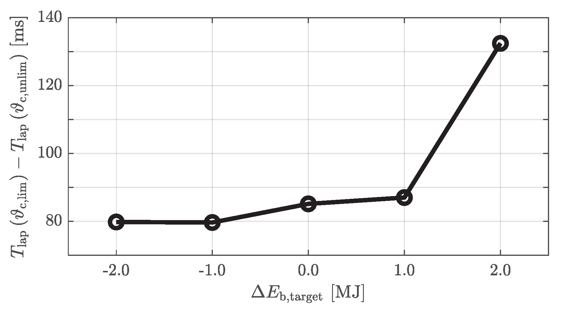
In Section 4.1 it was analyzed in detail how the compressor outlet temperature influences the achievable lap time. For this reason, the lap time losses over an entire lap for the limited compressor outlet temperature for five different battery recharge targets, are shown in Figure 15. The trend shows that irrespective of the battery recharge target, limiting the compressor outlet temperature can yield a significant lap time loss. This result clearly quantifies how lap time sensitive the choice of the compressor material or the intercooler design can be.
Figure 15.
Lap time losses over an entire lap for five different battery recharge targets with the same fuel consumption target and the limited compressor outlet temperature used in Section 4.1.
The average internal combustion engine and energy recovery system powers for different battery recharge targets but the same fuel target are shown in Figure 16. While the internal combustion engine and the energy recovery system powers in the corners influence the energy at disposal to the power unit when exiting the corners, they do not have a direct impact on the achievable lap time. For this reason, each power entry is averaged over all straights. The trends displayed in Figure 16 are in line with the ones seen in Section 4.1. The battery recharge target has an influence on the time interval the waste-gate is kept open, and therefore directly influences the resulting engine pumping power. The latter is shown to have the largest impact on the overall engine power, since the sum of the engine combustion and friction power are, on average, constant for all the battery budgets (for the considered fuel consumption target). Opening the waste-gate comes at the expense of a lower MGU-H recuperation: in fact, the average MGU-H recuperation (on straight) is roughly zero if the waste-gate is kept always open. A similar trend is observed for the MGU-K operation, whose average value becomes larger if more battery energy can be depleted. Overall, the power drawn from the battery, i.e., the sum of the MGU-K and MGU-H powers, becomes very small in magnitude if an aggressive battery recharge target has to be met: The power recuperated from the extra enthalpy contained in the hot exhaust gases is directly fed from the MGU-H to the MGU-K. From a lap time point of view, it can be noticed how the lap time sensitivity changes: the lap time loss from to is more than twice compared to the one from to . Among other effects this can be explained by the nonlinearity of the lap time integration in the objective and the longitudinal dynamics.
Figure 16.
Internal combustion engine powers, energy recovery system powers and times for 9 different battery recharge targets with the same fuel consumption target. The overhead bar stands for a variable that is averaged over all straights.
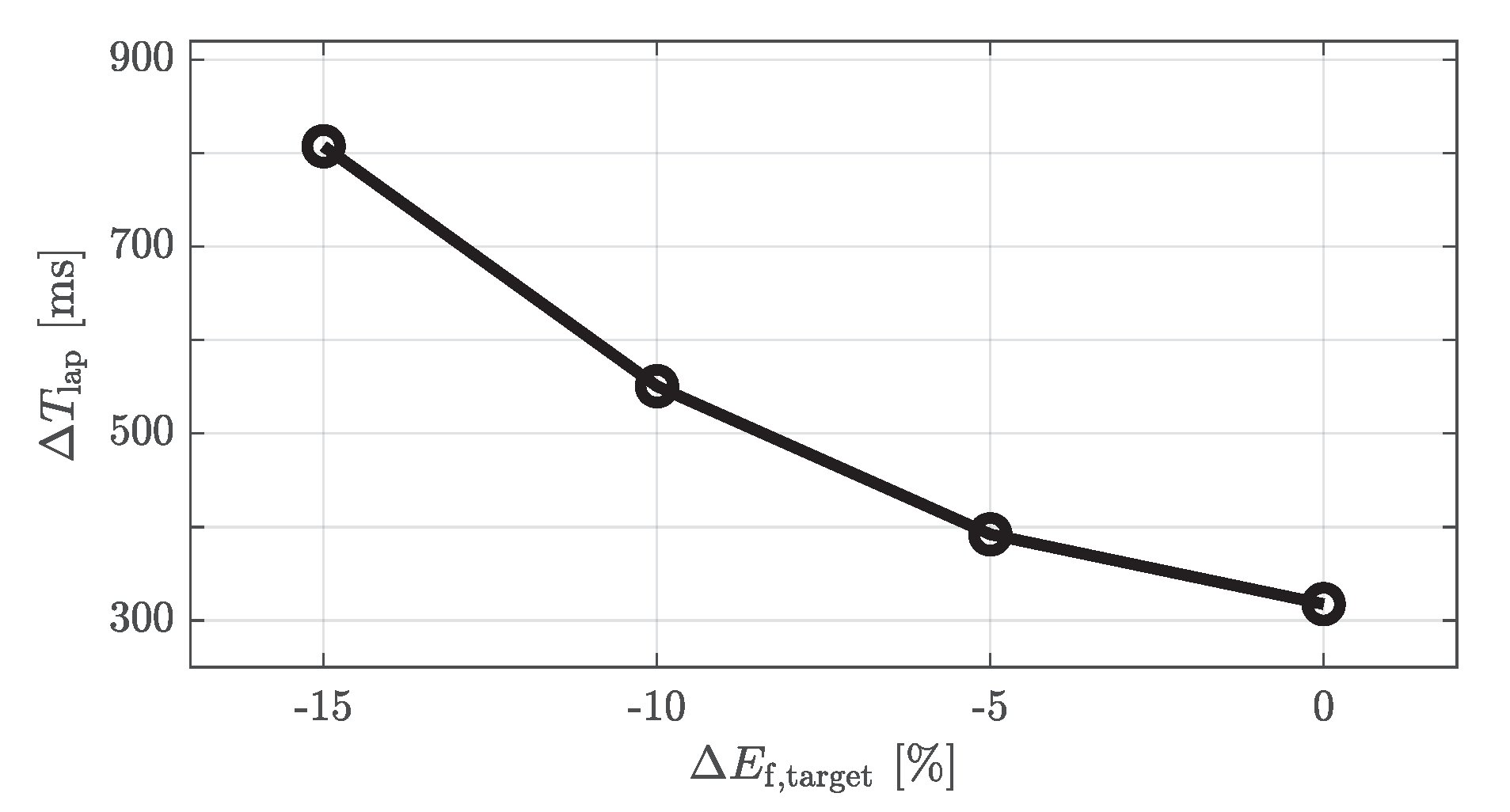
Finally, the lap time loss between and for several fuel consumption targets is shown in Figure 17. It can be noticed how the lap time loss increases nonlinearly if less fuel is used over the lap. This is a further proof of the complexity and inherent cross-couplings between the internal combustion engine and the energy recovery system of the considered hybrid electric powertrain.
Figure 17.
Lap time difference between and for four different fuel consumption targets. The reference fuel consumption target used is the same of Figure 16.
5. Conclusions
In this paper we presented an optimization framework to compute the time-optimal low-level control and gearshift strategies for the Formula 1 hybrid electric powertrain. We put the focus on the engine speed dependency of the internal combustion engine components and proposed a continuous nonlinear model to describe the engine cylinder deactivation. Furthermore, we applied convex relaxations to model the non-smooth maximum fuel mass flow regulation and captured the highly nonlinear turbocharger maps with neural network techniques. Finally, we solved the time-optimal control problem efficiently by applying outer convexification to the integer decision variable introduced by the gear selection. To showcase the optimization framework, we performed several case studies for different energy budgets. The results underlined the significant existing coupling between the internal combustion engine and the energy recovery system: The gearshift strategy, the MGU-K and MGU-H operation, the air-to-fuel ratio operational range, the waste-gate and throttle valve actuation, as well as the intake manifold pressure evolution were found to be strongly dependent on the energy budgets. Finally, we demonstrated the effectiveness of our framework as a design tool. For example, if the compressor outlet temperature has to be reduced by due to a change in the intercooler design, the lap time can increase by up to for the considered conditions. The results presented in this work underline that the framework can be used as a tool to benchmark real-time control strategies, to generate reference trajectories and to develop control heuristics.
Author Contributions
Conceptualization, C.B., M.-P.N., N.R., A.C. and V.R.; methodology, C.B., M.-P.N. and N.R.; software, C.B. and M.-P.N.; validation, C.B. and M.-P.N.; formal analysis, C.B. and M.-P.N.; investigation, C.B. and M.-P.N.; resources, C.B., M.-P.N., A.C. and V.R.; data curation, C.B., M.-P.N. and P.D.; writing–original draft preparation, C.B. and M.-P.N.; writing–review and editing, C.B., M.-P.N. and N.R., P.D., A.C. and C.O.; visualization, C.B., M.-P.N. and P.D.; supervision, A.C. and C.O.; project administration, C.O.; funding acquisition, C.O. All authors have read and agreed to the published version of the manuscript.
Funding
This research was funded by Ferrari S.p.A.
Institutional Review Board Statement
Not applicable.
Informed Consent Statement
Not applicable.
Data Availability Statement
Not applicable.
Acknowledgments
We would like to thank Ferrari S.p.A. for supporting this project. Moreover, we would like to express our gratitude to Ilse New for her helpful and valuable comments during the proofreading phase. Last, but not least, we would like to acknowledge Ristorante Montana for the support and the inspiration.
Conflicts of Interest
The authors declare that they have no known competing financial interests or personal relationships that could have appeared to influence the work reported in this paper.
Appendix A. Optimal Control Problem (Outer Convexified Formulation)
In this section, we state the optimal control problem. The state x and input u variables are
The resulting time-optimal low-level optimization problem is
subject to the dynamics
the system equality constraints
the system inequality constraints related to the integer variables
the system inequality constraints
and the initial and terminal constraints
where , , , , and are the initial and terminal conditions for the velocity of the car, the intake manifold pressure and the turbocharger kinetic energy, respectively. For periodic paths (e.g., entire lap optimizations where the start and finish line coincide), the last six constraints of Equation (A7) can be rewritten as periodicity conditions, i.e.,
and can be freely optimized.
Appendix B. Mixed-Integer Nonlinear Program Solution
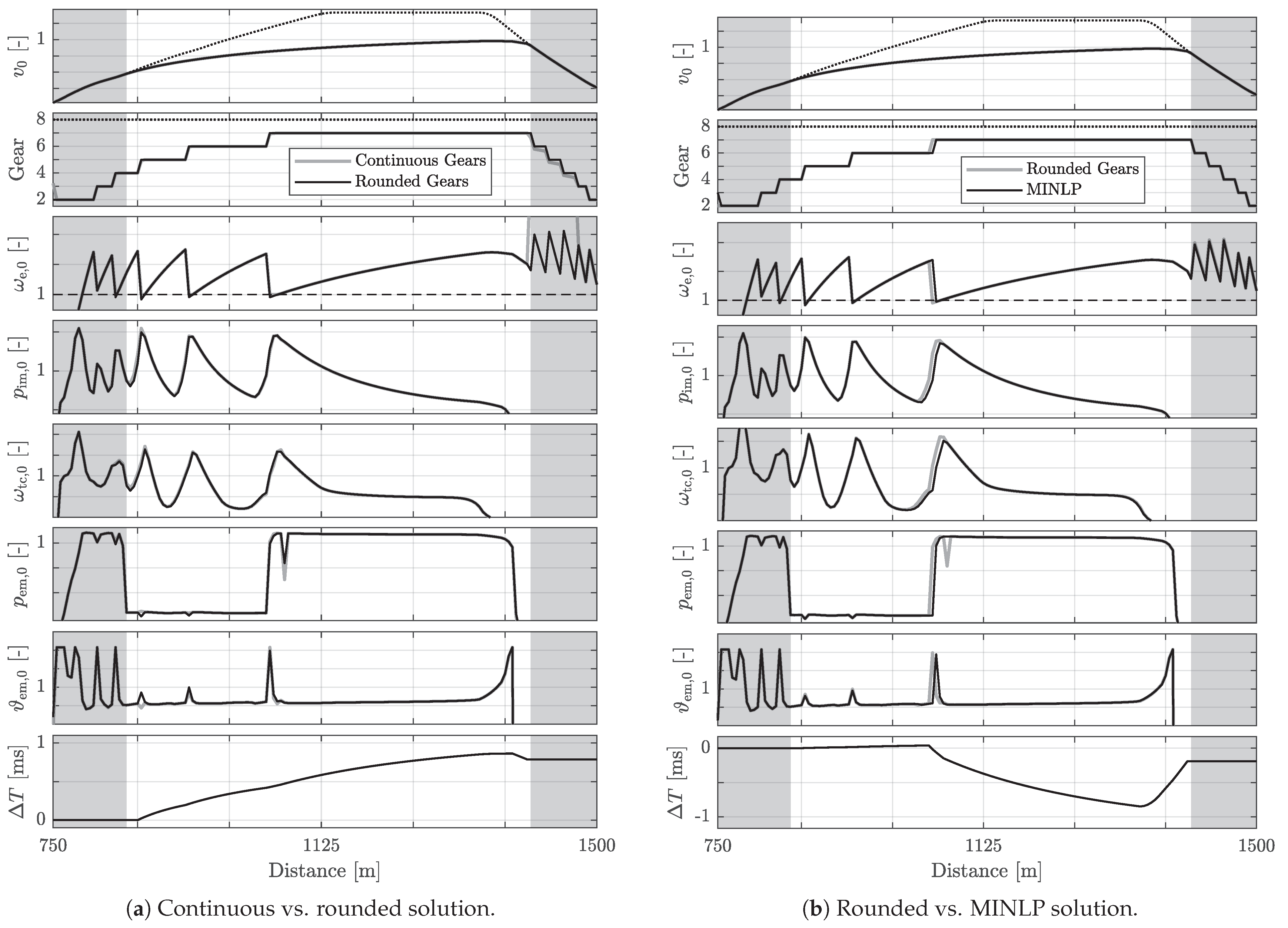
In this section, we present a comparison between the continuous solution, the rounded solution and the mixed-integer nonlinear program (MINLP) solution. The results are shown in Figure A1. As can be seen, the continuous solution partially differs from the rounded one. The gear trajectories are close to each other except in the braking phase of the second corner. Despite this fact, the difference between the solutions is marginal and the overall lap time difference is less than . Except for one point where the gearshift occurs one space step earlier, the rounded and the MINLP solutions are similar. This results in a lap time difference of less than . Given that the optimization of the continuous and rounded NLPs together displays computational times more than 100 times faster than the MINLP optimization, we deem the small difference acceptable.
Figure A1.
Optimal state and input trajectories over a straight and a corner for the same battery and fuel budgets: (a) continuous vs. rounded solution, (b) rounded vs. MINLP solution. The dotted lines are the state and input limits, while the dashed line in the engine speed plot is placed at .
Appendix C. Neural Networks
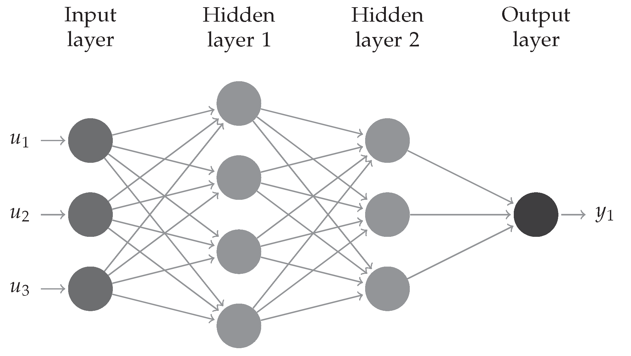
This Appendix is based on [47] and briefly summarizes the methodology used to fit the maps presented in Section 2. We apply feedforward neural networks. More precisely, we focus only on regression, i.e., both the input and output vectors consist of real numbers, where .
Figure A2.
Feedforward neural network schematic taken from [47]. The structure consists of hidden layers, inputs and output. Each neuron is connected to the next ones through arrows.
As shown in Figure A2, neural networks are structured in layers, each consisting of multiple nodes. In particular, our architecture is composed of the input layer, where each node stores the s-th entry of the input vector u, with , hidden layers, where each node is fed with all output information of the previous layer, and the output layer, that collects the information of the L-th hidden layer and generates a prediction. More precisely, each node of layer performs following operation:
where denotes the number of nodes of layer k, is the node’s internal variable, and denotes its output. The activation function of layer k can be chosen arbitrarily. In this work we choose the hyperbolic tangent function
for the hidden layers to increase the fitting quality of the nonlinear maps, and a linear function for the output layer. Finally, the parameters and are learned during the training phase. It consists of determining the set of parameters which minimizes a loss function over a given dataset . Specifically, let be the mapping described by the feedforward neural network. By applying a squared loss function, it follows that
The optimization methodology used does not guarantee global optimality of the solution. Therefore it is important to check the quality of the fitting a posteriori.
References
- FIA. 2018 Formula One Sporting Regulations; Technical Report; FIA: Geneva, Switzerland, 2018. [Google Scholar]
- FIA. 2018 Formula One Technical Regulations; Technical Report; FIA: Geneva, Switzerland, 2018. [Google Scholar]
- Hooker, J. Optimal driving for single-vehicle fuel economy. Transp. Res. Part A Gen. 1988, 22, 183–201. [Google Scholar] [CrossRef]
- Pérez, L.V.; Pilotta, E.A. Optimal power split in a hybrid electric vehicle using direct transcription of an optimal control problem. Math. Comput. Simul. 2009, 79, 1959–1970. [Google Scholar] [CrossRef]
- Heppeler, G.; Sonntag, M.; Sawodny, O. Fuel efficiency analysis for simultaneous optimization of the velocity trajectory and the energy management in hybrid electric vehicles. IFAC Proc. Vol. 2014, 47, 6612–6617. [Google Scholar] [CrossRef]
- Sciarretta, A.; Back, M.; Guzzella, L. Optimal control of parallel hybrid electric vehicles. IEEE Trans. Control. Syst. Technol. 2004, 12, 352–363. [Google Scholar] [CrossRef]
- Elbert, P.; Nüesch, T.; Ritter, A.; Murgovski, N.; Guzzella, L. Engine on/off control for the energy management of a serial hybrid electric bus via convex optimization. IEEE Trans. Veh. Technol. 2014, 63, 3549–3559. [Google Scholar] [CrossRef]
- Nüesch, T.; Elbert, P.; Flankl, M.; Onder, C.; Guzzella, L. Convex optimization for the energy management of hybrid electric vehicles considering engine start and gearshift costs. Energies 2014, 7, 834–856. [Google Scholar] [CrossRef]
- Sciarretta, A.; Guzzella, L. Control of hybrid electric vehicles. Control Syst. IEEE 2007, 27, 60–70. [Google Scholar]
- Kim, N.; Cha, S.; Peng, H. Optimal control of hybrid electric vehicles based on Pontryagin’s minimum principle. IEEE Trans. Control. Syst. Technol. 2011, 19, 1279–1287. [Google Scholar]
- Sciarretta, A.; De Nunzio, G.; Ojeda, L.L. Optimal Ecodriving Control: Energy-Efficient Driving of Road Vehicles as an Optimal Control Problem. Control Syst. IEEE 2015, 35, 71–90. [Google Scholar]
- Murgovski, N.; Johannesson, L.; Sjöberg, J.; Egardt, B. Component sizing of a plug-in hybrid electric powertrain via convex optimization. Mechatronics 2012, 22, 106–120. [Google Scholar] [CrossRef]
- Ebbesen, S.; Dönitz, C.; Guzzella, L. Particle Swarm Optimization for Hybrid Electric Drive-train Sizing. Int. J. Veh. Des. 2012, 58, 181–199. [Google Scholar] [CrossRef]
- Ebbesen, S.; Elbert, P.; Guzzella, L. Engine Downsizing and Electric Hybridization Under Consideration of Cost and Drivability. Oil Gas Sci. Technol.-Rev. IFP Energies Nouv. 2012, 68, 109–116. [Google Scholar] [CrossRef]
- Wijkniet, J.; Hofman, T. Modified computational design synthesis using simulation-based evaluation and constraint consistency for vehicle powertrain systems. IEEE Trans. Veh. Technol. 2018, 67, 8065–8076. [Google Scholar] [CrossRef]
- Paganelli, G.; Delprat, S.; Guerra, T.M.; Rimaux, J.; Santin, J.J. Equivalent consumption minimization strategy for parallel hybrid powertrains. In Proceedings of the Vehicular Technology Conference, 2002. VTC Spring 2002, Birmingham, AL, USA, 6–9 May 2002; pp. 2076–2081. [Google Scholar]
- Serrao, L.; Onori, S.; Rizzoni, G. A comparative analysis of energy management strategies for hybrid electric vehicles. J. Dyn. Syst. Meas. Control 2011, 133, 1–9. [Google Scholar] [CrossRef]
- Nüesch, T.; Cerofolini, A.; Mancini, G.; Cavina, N.; Onder, C.; Guzzella, L. Equivalent consumption minimization strategy for the control of real driving NOx emissions of a diesel hybrid electric vehicle. Energies 2014, 7, 3148–3178. [Google Scholar] [CrossRef]
- Ebbesen, S.; Elbert, P.; Guzzella, L. Battery state-of-health perceptive energy management for hybrid electric vehicles. IEEE Trans. Veh. Technol. 2012, 61, 2893–2900. [Google Scholar] [CrossRef]
- Zhao, D.; Stobart, R.; Dong, G.; Winward, E. Real-time energy management for diesel heavy duty hybrid electric vehicles. IEEE Trans. Control. Syst. Technol. 2015, 23, 829–841. [Google Scholar] [CrossRef]
- Zhao, D.; Winward, E.; Yang, Z.; Stobart, R.; Steffen, T. Characterisation, control, and energy management of electrified turbocharged diesel engines. Energy Convers. Manag. 2017, 135, 416–433. [Google Scholar] [CrossRef]
- Schmid, R.; Bürger, J.; Bajcinca, N. Efficient optimal control of plug-in-hybrid electric vehicles including explicit engine on/off decisions. In Proceedings of the 2018 European Control Conference (ECC), Limassol, Cyprus, 12–15 June 2018; pp. 596–601. [Google Scholar]
- Ngo, V.; Hofman, T.; Steinbuch, M.; Serrarens, A. Optimal Control of the Gearshift Command for Hybrid Electric Vehicles. IEEE Trans. Veh. Technol. 2012, 61, 3531–3543. [Google Scholar] [CrossRef]
- Joševski, M.; Abel, D. Gear shifting and engine on/off optimal control in hybrid electric vehicles using partial outer convexification. In Proceedings of the 2016 IEEE Conference on Control Applications (CCA), Buenos Aires, Argentina, 19–22 September 2016; pp. 562–568. [Google Scholar]
- Joševski, M.; Abel, D. Distributed predictive control approach for fuel efficient gear shifting in hybrid electric vehicles. In Proceedings of the 2016 European Control Conference (ECC), Aalborg, Denmark, 29 June–1 July 2016; pp. 2366–2373. [Google Scholar]
- Kirches, C.; Bock, H.G.; Schlöder, J.P.; Sager, S. Mixed-integer NMPC for predictive cruise control of heavy-duty trucks. In Proceedings of the 2013 European Control Conference (ECC), Zurich, Switzerland, 17–19 July 2013; pp. 4118–4123. [Google Scholar]
- Kirches, C.; Sager, S.; Bock, H.G.; Schlöder, J.P. Time-optimal control of automobile test drives with gear shifts. Optim. Control. Appl. Methods 2010, 31, 137–153. [Google Scholar] [CrossRef]
- Robuschi, N.; Zeile, C.; Sager, S.; Braghin, F. Multiphase mixed-integer nonlinear optimal control of hybrid electric vehicles. Automatica 2021, 123, 109325. [Google Scholar] [CrossRef]
- Ritzmann, J.; Christon, A.; Salazar, M.; Onder, C.H. Fuel-optimal Power Split and Gear Selection Strategies for a Hybrid Electric Vehicle. In Proceedings of the SAE International Conference on Engines & Vehicles, Capri, Italy, 15–19 September 2019. [Google Scholar]
- Robuschi, N.; Salazar, M.; Duhr, P.; Braghin, F.; Onder, C.H. Minimum-fuel engine on/off control for the energy management of a hybrid electric vehicle via iterative linear programming. IFAC-PapersOnLine 2019, 52, 134–140. [Google Scholar] [CrossRef]
- Guzzella, L.; Onder, C.H. Introduction to Modeling and Control of Internal Combustion Engine Systems, 2nd ed.; Springer: Berlin/Heidelberg, Germany, 2010. [Google Scholar]
- Eriksson, L. Modeling and control of turbocharged SI and DI engines. Oil Gas Sci. Technol.-Rev. l’IFP 2007, 62, 523–538. [Google Scholar] [CrossRef]
- Eriksson, L.; Nielsen, L. Modeling and Control of Engines and Drivelines; John Wiley & Sons: Hoboken, NJ, USA, 2014. [Google Scholar]
- Arsie, I.; Pianese, C.; Rizzo, G.; Flora, R.; Serra, G. A computer code for SI engine control and powertrain simulation. SAE Trans. 2000, 114, 935–949. [Google Scholar]
- Asprion, J.; Chinellato, O.; Guzzella, L. Optimisation-oriented modelling of the NOx emissions of a diesel engine. Energy Convers. Manag. 2013, 75, 61–73. [Google Scholar] [CrossRef]
- Asprion, J.; Chinellato, O.; Guzzella, L. Optimal control of diesel engines: Numerical methods, applications, and experimental validation. Math. Probl. Eng. 2014, 2014, 1–21. [Google Scholar] [CrossRef] [PubMed]
- Ekberg, K.; Leek, V.; Eriksson, L. Optimal control of wastegate throttle and fuel injection for a heavy-duty turbocharged diesel engine during tip-in. In Proceedings of the 58th Conference on Simulation and Modelling (SIMS 58), Reykjavik, Iceland, 25–27 September 2017; Linköping University Electronic Press: Linköping, Sweden, 2017; pp. 317–325. [Google Scholar]
- Eriksson, L.; Frei, S.; Onder, C.; Guzzella, L. Control and optimization of turbocharged spark ignited engines. IFAC Proc. Vol. 2002, 35, 283–288. [Google Scholar] [CrossRef]
- Sivertsson, M.; Eriksson, L. Modeling for optimal control: A validated diesel-electric powertrain model. In SIMS 2014-55th International Conference on Simulation and Modelling; Linköping University Electronic Press: Linköping, Sweden, 2014; pp. 49–58. [Google Scholar]
- Eriksson, L.; Nielsen, L.; Brugård, J.; Bergström, J.; Pettersson, F.; Andersson, P. Modeling of a turbocharged SI engine. Annu. Rev. Control 2002, 26, 129–137. [Google Scholar] [CrossRef]
- Keller, M.; Geiger, S.; Günther, M.; Pischinger, S.; Abel, D.; Albin, T. Model predictive air path control for a two-stage turbocharged spark-ignition engine with low pressure exhaust gas recirculation. Int. J. Engine Res. 2020, 21, 1835–1845. [Google Scholar] [CrossRef]
- Albin, T.; Ritter, D.; Liberda, N.; Quirynen, R.; Diehl, M. In-vehicle realization of nonlinear MPC for gasoline two-stage turbocharging airpath control. IEEE Trans. Control Syst. Technol. 2017, 26, 1606–1618. [Google Scholar] [CrossRef]
- Dickinson, P.; Glover, K.; Collings, N.; Yamashita, Y.; Yashiro, Y.; Hoshi, T. Real-time control of a two-stage serial VGT diesel engine using MPC. IFAC-PapersOnLine 2015, 48, 117–123. [Google Scholar] [CrossRef]
- Herceg, M.; Raff, T.; Findeisen, R.; Allgowe, F. Nonlinear model predictive control of a turbocharged diesel engine. In Proceedings of the 2006 IEEE Conference on Computer Aided Control System Design, 2006 IEEE International Conference on Control Applications, 2006 IEEE International Symposium on Intelligent Control, Munich, Germany, 4–6 October 2006; pp. 2766–2771. [Google Scholar]
- Marinkov, S.; Murgovski, N.; de Jager, B. Convex modeling and sizing of electrically supercharged internal combustion engine powertrain. IEEE Trans. Veh. Technol. 2016, 65, 4523–4534. [Google Scholar] [CrossRef]
- Marinkov, S.; Murgovski, N.; de Jager, B. Convex Modeling and Optimization of a Vehicle Powertrain Equipped With a Generator–Turbine Throttle Unit. IEEE Trans. Control. Syst. Technol. 2017, 25, 1264–1277. [Google Scholar] [CrossRef]
- Balerna, C.; Lanzetti, N.; Salazar, M.; Cerofolini, A.; Onder, C. Optimal low-level control strategies for a high-performance hybrid electric power unit. Appl. Energy 2020, 276, 115248. [Google Scholar] [CrossRef]
- Casanova, D. On Minimum Time Vehicle Manoeuvring: The Theoretical Optimal Lap. Ph.D. Thesis, School of Mechanical Engineering, Cranfield University, Bedford, UK, 2000. [Google Scholar]
- Perantoni, G.; Limebeer, D. Optimal control for a formula one car with variable parameters. Veh. Syst. Dyn. 2014, 52, 653–678. [Google Scholar] [CrossRef]
- Limebeer, D.; Perantoni, G. Optimal control of a formula one car on a three-dimensional track—Part 2: Optimal control. J. Dyn. Syst. Meas. Control 2015, 137. [Google Scholar] [CrossRef]
- Masouleh, M.I.; Limebeer, D.J. Optimizing the Aero-Suspension Interactions in a Formula One Car. IEEE Trans. Control. Syst. Technol. 2016, 24, 912–927. [Google Scholar] [CrossRef]
- Tremlett, A.J.; Limebeer, D.J.N. Optimal tyre usage for a Formula One car. Veh. Syst. Dyn. 2016, 54, 1448–1473. [Google Scholar] [CrossRef]
- Lot, R.; Evangelou, S. Lap time optimization of a sports series hybrid electric vehicle. In Proceedings of the 2013 World Congress on Engineering, London, UK, 3–5 July 2013; pp. 1–6. [Google Scholar]
- Limebeer, D.; Perantoni, G.; Rao, A. Optimal control of Formula One car energy recovery systems. Int. J. Control 2014, 87, 2065–2080. [Google Scholar] [CrossRef]
- Liu, X.; Fotouhi, A.; Auger, D.J. Optimal energy management for formula-E cars with regulatory limits and thermal constraints. Appl. Energy 2020, 279, 115805. [Google Scholar] [CrossRef]
- Herrmann, T.; Passigato, F.; Betz, J.; Lienkamp, M. Minimum Race-Time Planning-Strategy for an Autonomous Electric Racecar. arXiv 2020, arXiv:2005.07127. [Google Scholar]
- Ebbesen, S.; Salazar, M.; Elbert, P.; Bussi, C.; Onder, C.H. Time-optimal control strategies for a hybrid electric race car. IEEE Trans. Control Syst. Technol. 2018, 26, 233–247. [Google Scholar] [CrossRef]
- Salazar, M.; Elbert, P.; Ebbesen, S.; Bussi, C.; Onder, C.H. Time-optimal control policy for a hybrid electric race car. IEEE Trans. Control Syst. Technol. 2017, 25, 1921–1934. [Google Scholar] [CrossRef]
- Salazar, M.; Balerna, C.; Chisari, E.; Bussi, C.; Onder, C.H. Equivalent lap time minimization strategies for a hybrid electric race car. In Proceedings of the 2018 IEEE Conference on Decision and Control (CDC), Miami Beach, FL, USA, 17–19 December 2018; pp. 6125–6131. [Google Scholar]
- Salazar, M.; Duhr, P.; Balerna, C.; Arzilli, L.; Onder, C.H. Minimum lap time control of hybrid electric race cars in qualifying scenarios. IEEE Trans. Veh. Technol. 2019, 68, 7296–7308. [Google Scholar] [CrossRef]
- Balerna, C.; Salazar, M.; Lanzetti, N.; Bussi, C.; Onder, C.H. Adaptation Algorithms for the Hybrid Electric Powertrain of a Race Car. In Proceedings of the FISITA World Automotive Congress, Chennai, India, 2–5 October 2018. [Google Scholar]
- Salazar, M.; Balerna, C.; Elbert, P.; Grando, F.P.; Onder, C.H. Real-Time Control Algorithms for a Hybrid Electric Race Car Using a Two-Level Model Predictive Control Scheme. IEEE Trans. Veh. Technol. 2017, 66, 10911–10922. [Google Scholar] [CrossRef]
- Duhr, P.; Christodoulou, G.; Balerna, C.; Salazar, M.; Cerofolini, A.; Onder, C.H. Time-optimal Gearshift and Energy Management Strategies for a Hybrid Electric Race Car. Appl. Energy 2020, 282, 115980. [Google Scholar] [CrossRef]
- Hoheisel, T.; Kanzow, C.; Schwartz, A. Theoretical and numerical comparison of relaxation methods for mathematical programs with complementarity constraints. Math. Program. 2013, 137, 257–288. [Google Scholar] [CrossRef]
- Eriksson, L. Mean value models for exhaust system temperatures. SAE Trans. 2002, 111, 753–767. [Google Scholar]
- Roeth, J.; Guzzella, L. Modelling engine and exhaust temperatures of a mono-fuelled turbocharged compressed-natural-gas engine during warm-up. Proc. Inst. Mech. Eng. Part D J. Automob. Eng. 2010, 224, 99–115. [Google Scholar] [CrossRef]
- Fiengo, G.; Glielmo, L.; Santini, S.; Serra, G. Control oriented models for twc-equipped spark ignition engines during the warm-up phase. In Proceedings of the 2002 American Control Conference (IEEE Cat. No. CH37301), Anchorage, AK, USA, 8–10 May 2002; pp. 1761–1766. [Google Scholar]
- Egardt, B.; Murgovski, N.; Pourabdollah, M.; Mardh, L.J. Electromobility studies based on convex optimization: Design and control issues regarding vehicle electrification. IEEE Control Syst. 2014, 34, 32–49. [Google Scholar]
- Murgovski, N.; Johannesson, L.M.; Sjöberg, J. Engine on/off control for dimensioning hybrid electric powertrains via convex optimization. IEEE Trans. Veh. Technol. 2013, 62, 2949–2962. [Google Scholar] [CrossRef]
- Till, J.; Engell, S.; Panek, S.; Stursberg, O. Applied hybrid system optimization: An empirical investigation of complexity. Control Eng. Pract. 2004, 12, 1291–1303. [Google Scholar] [CrossRef]
- Sager, S. Numerical Methods for Mixed-Integer Optimal Control Problems; Der Andere Verlag: Tönning, Germany, 2005. [Google Scholar]
- Jung, M. Relaxations and Approximations for Mixed-Integer Optimal Control. Ph.D. Thesis, Ruprecht Karls Universtät, Heidelberg, Germany, 2014. [Google Scholar]
- Kirches, C. Fast Numerical Methods for Mixed-Integer Nonlinear Model-Predictive Control; Springer: Berlin/Heidelberg, Germany, 2011. [Google Scholar]
- Sager, S.; Bock, H.G.; Diehl, M. Solving Mixed–integer Control Problems by Sum Up Rounding With Guaranteed Integer Gap. SIAM J. Control Optim. 2007. [Google Scholar] [CrossRef]
- MATLAB. Version 7.10.0 (R2010a); The MathWorks Inc.: Natick, MA, USA, 2010. [Google Scholar]
- Andersson, J.A.E.; Gillis, J.; Horn, G.; Rawlings, J.B.; Diehl, M. CasADi—A software framework for nonlinear optimization and optimal control. Math. Program. Comput. 2019, 11, 1–36. [Google Scholar] [CrossRef]
- Wächter, A.; Biegler, L.T. On the implementation of an interior-point filter line-search algorithm for large-scale nonlinear programming. Math. Program. 2006, 106, 25–57. [Google Scholar] [CrossRef]
- Bonami, P.; Biegler, L.T.; Conn, A.R.; Cornuéjols, G.; Grossmann, I.E.; Laird, C.D.; Lee, J.; Lodi, A.; Margot, F.; Sawaya, N.; et al. An algorithmic framework for convex mixed integer nonlinear programs. Discret. Optim. 2008, 5, 186–204. [Google Scholar] [CrossRef]
- Thomasson, A.; Eriksson, L.; Leufven, O.; Andersson, P. Wastegate actuator modeling and model-based boost pressure control. IFAC Proc. Vol. 2009, 42, 87–94. [Google Scholar] [CrossRef]
Publisher’s Note: MDPI stays neutral with regard to jurisdictional claims in published maps and institutional affiliations. |
© 2020 by the authors. Licensee MDPI, Basel, Switzerland. This article is an open access article distributed under the terms and conditions of the Creative Commons Attribution (CC BY) license (http://creativecommons.org/licenses/by/4.0/).