Fast and Robust Hybrid Starter and Generator Speed Control for Improving Drivability of Parallel Hybrid Electric Vehicles


Abstract
:1. Introduction
- (1)
- When the step speed command is applied, speed overshoot and steady-state errors scarcely occur. Since the speed command tracking performance is similar to that of a first-order low-pass filter (LPF), the proposed controller can be designed by predicting the control performance using the time constant concept when designing the control performance.
- (2)
- When the ramp speed command is applied, it results in a very small steady-state error. Since forward compensation for the command is used, it does not react to speed measurement noise applied through the feedback loop of the speed controller. The forward compensator is based on an inverse function of the speed controller; therefore, the gain design of the forward compensator is simple.
- (3)
- The proposed speed control method is resilient to parameter variations, such as the moment of inertia and the viscous friction coefficient required for controller design. Even if parameter variation occurs, the effect on the designed control bandwidth is small, and the steady-state error for step or ramp commands is small.
- (4)
- The variation in speed is small as the proposed method uses a structure that increases the damping of the entire system using the speed for feedback even if an uncertain disturbance is encountered.
- (5)
- A method of designing the controller gain considering the constraints of the system is presented. When limiting the rate of change of torque to prevent belt slip in order to guarantee the durability of the system (connected by belt), a method for designing a control gain considering the rate of change of torque and disturbance type is presented.
2. Preliminaries
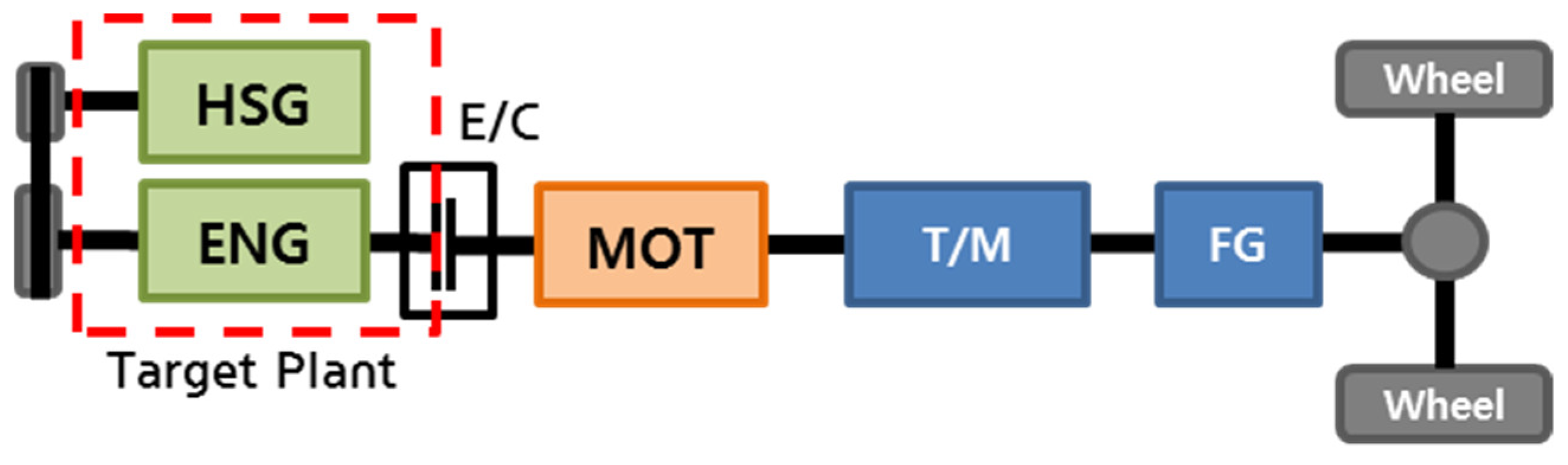
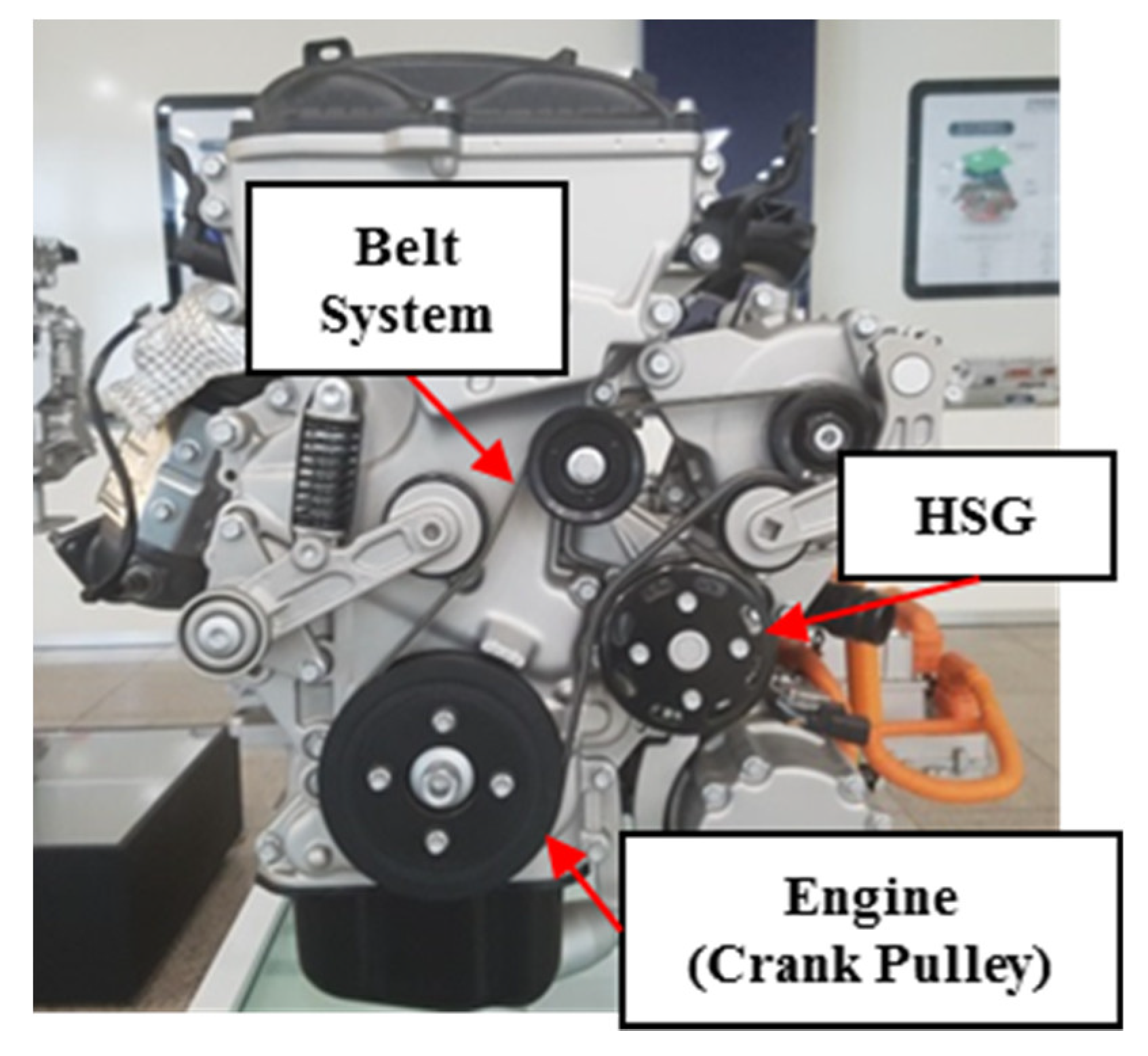
2.1. Outline and Features of TMED Systems
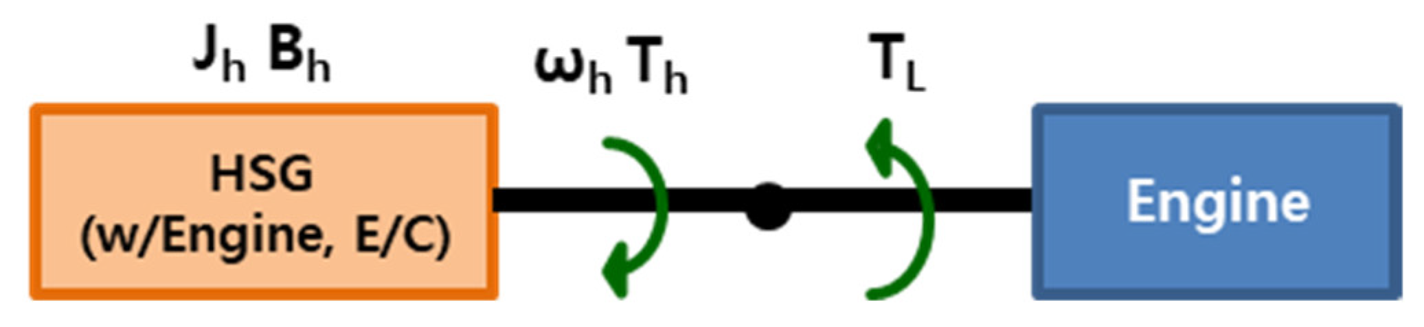
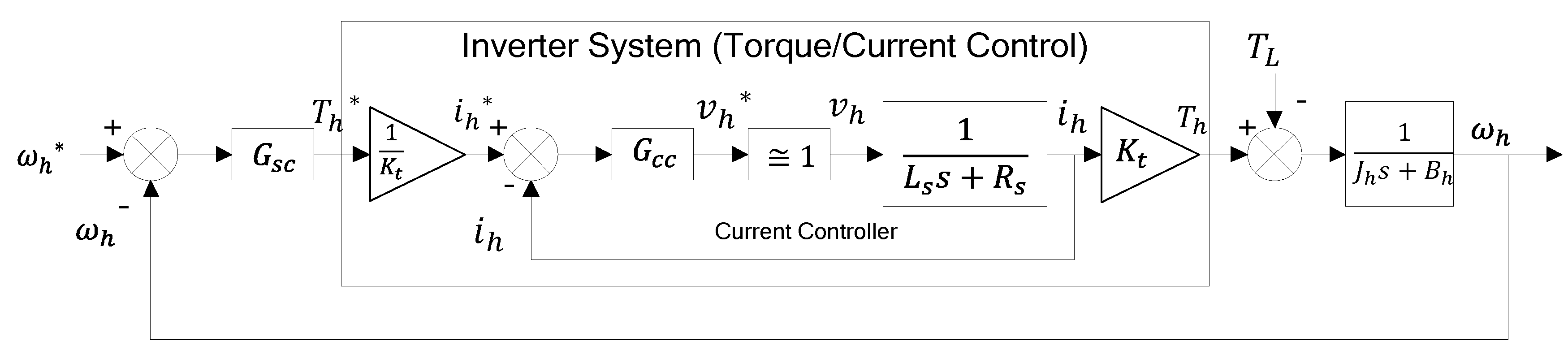
2.2. Mathematical Model of HSG
3. Design of Speed Controller
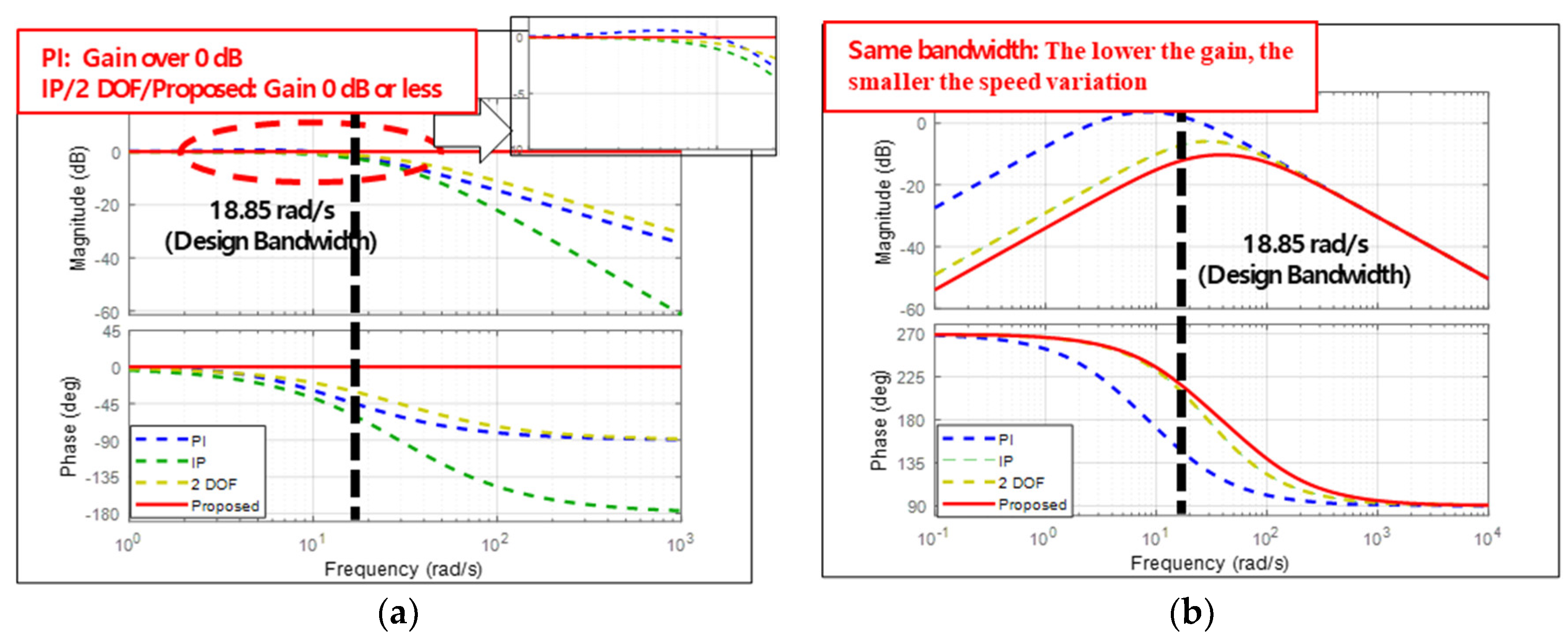
3.1. Conventional Speed Controllers
3.2. Proposed Speed Controller
3.3. Design of the Proposed Controller Gain
- (1)
- In the entire control system, if the current (torque) controller control bandwidth of the inner loop is more than ten times greater than that of the outer loop speed controller, the output of the current controller has a very small effect on the speed controller and can be ignored. If the control bandwidth of the current controller operating in the inner loop is 200 Hz, the control bandwidth of the speed controller operating in the outer loop must satisfy the condition of 20 Hz or less. However, since the 1st LPF with a cut-off frequency of 20 Hz is used to block noise at the HSG speeds used as the speed controller inputs, the control bandwidth was designed to be less than 1/5 of the filter cut-off frequency to minimize the effect of the filter. Considering all the above, the control bandwidth of the speed controller can be selected to be 4 Hz or less—herein, it was designed to be 3 Hz, to simulate and test the vehicle.
- (2)
- The control gain of the active damping controller should be designed in consideration of the limitations on the output torque of the HSG (maximum output, maximum torque, output torque change rate, etc.) and the output characteristics of the engine operating under load. The characteristics to be considered in particular are the constraints limiting the change rate of HSG output torque to prevent belt slip occurrence and the magnitude of HSG speed variation owing to C2 oscillations having twice the frequency of engine rotation produced by the operating characteristics of the engine. The time constant of the mechanical system represented by Equation (16) can be determined using the designed active damping coefficient.
4. Simulation Results
4.1. Frequency Domain Analysis
4.2. Time Domain Analysis
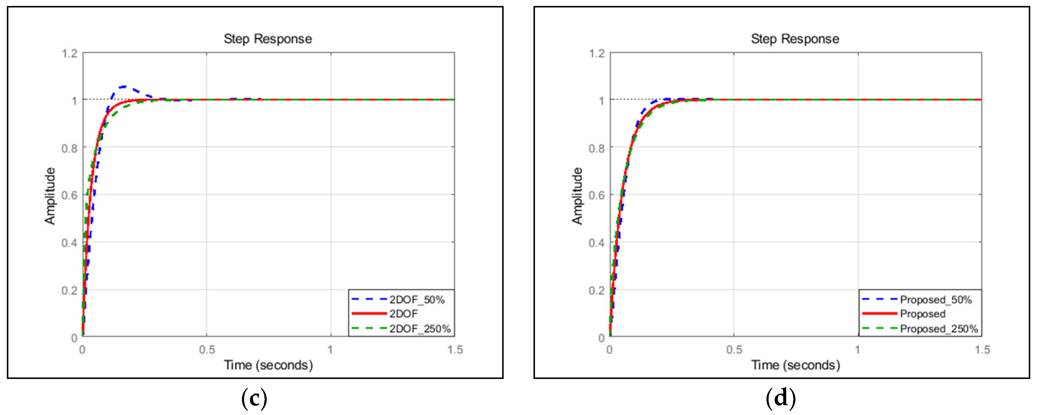
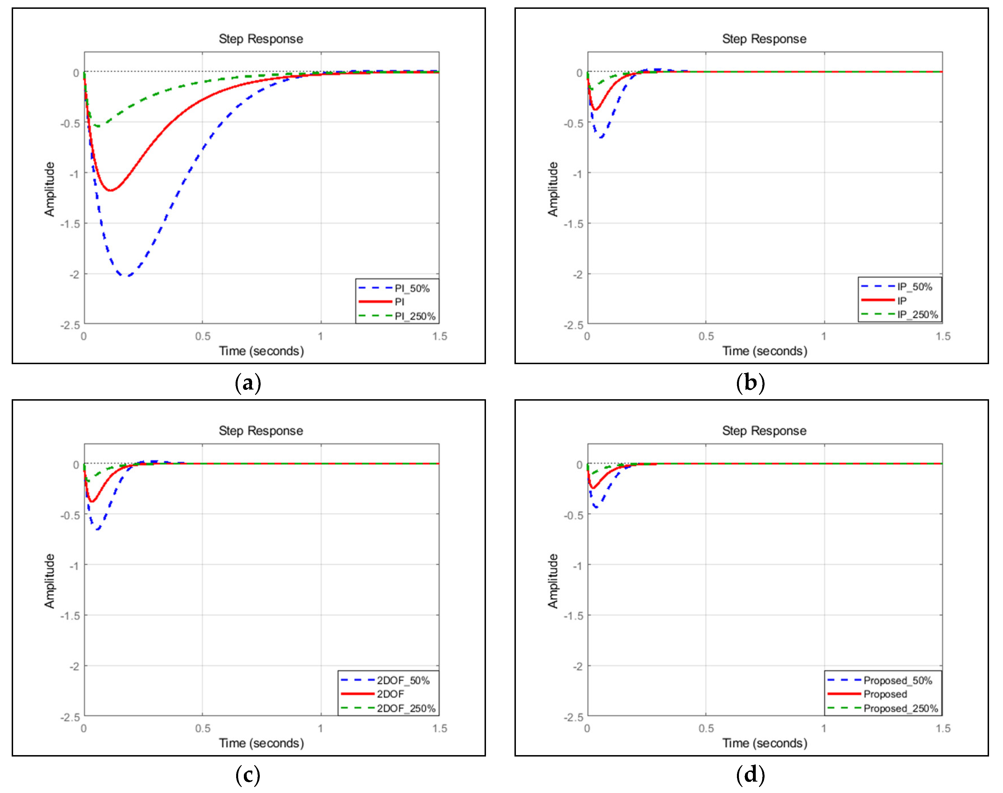
4.3. Robustness Analysis
5. Vehicle Test Results
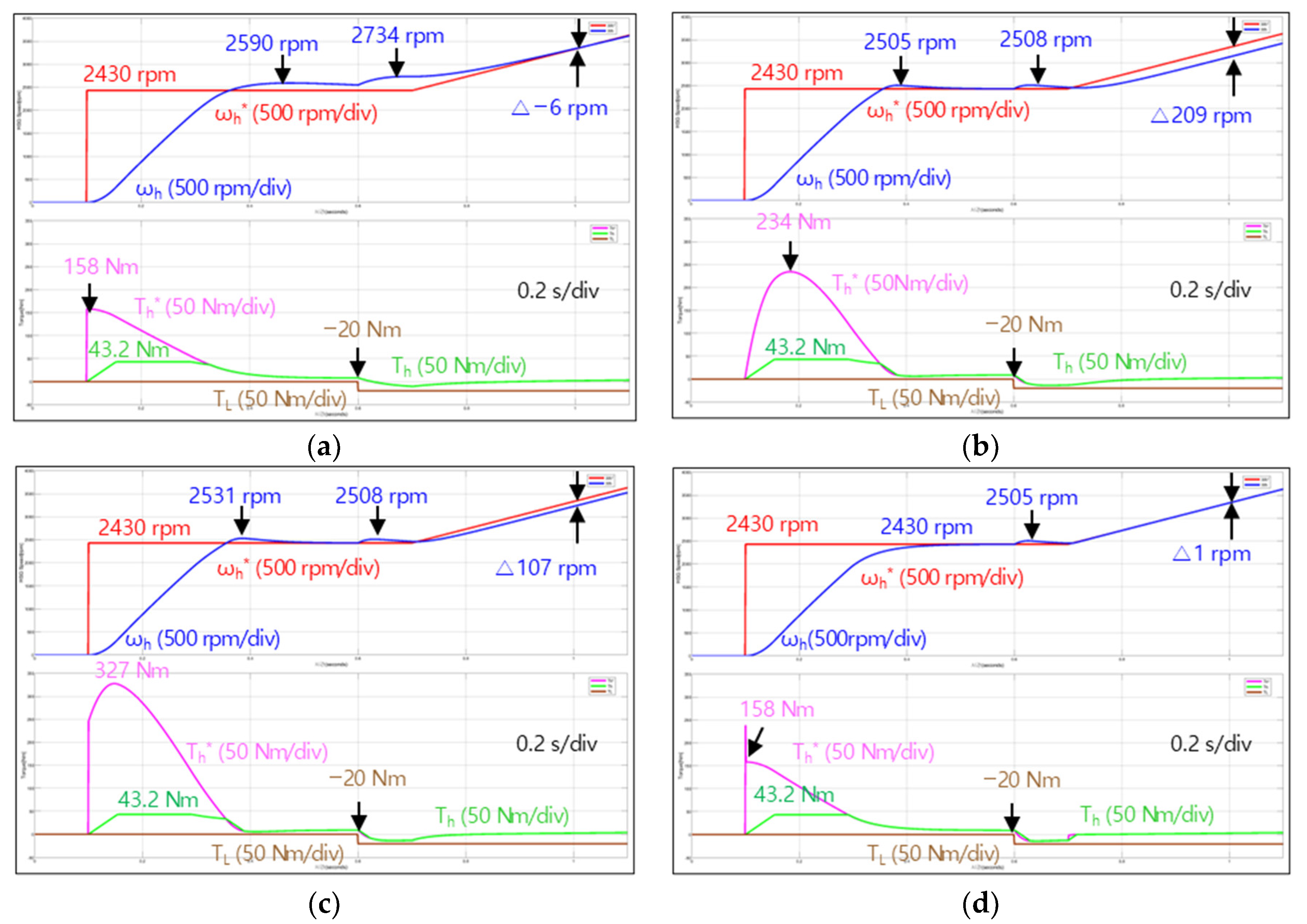
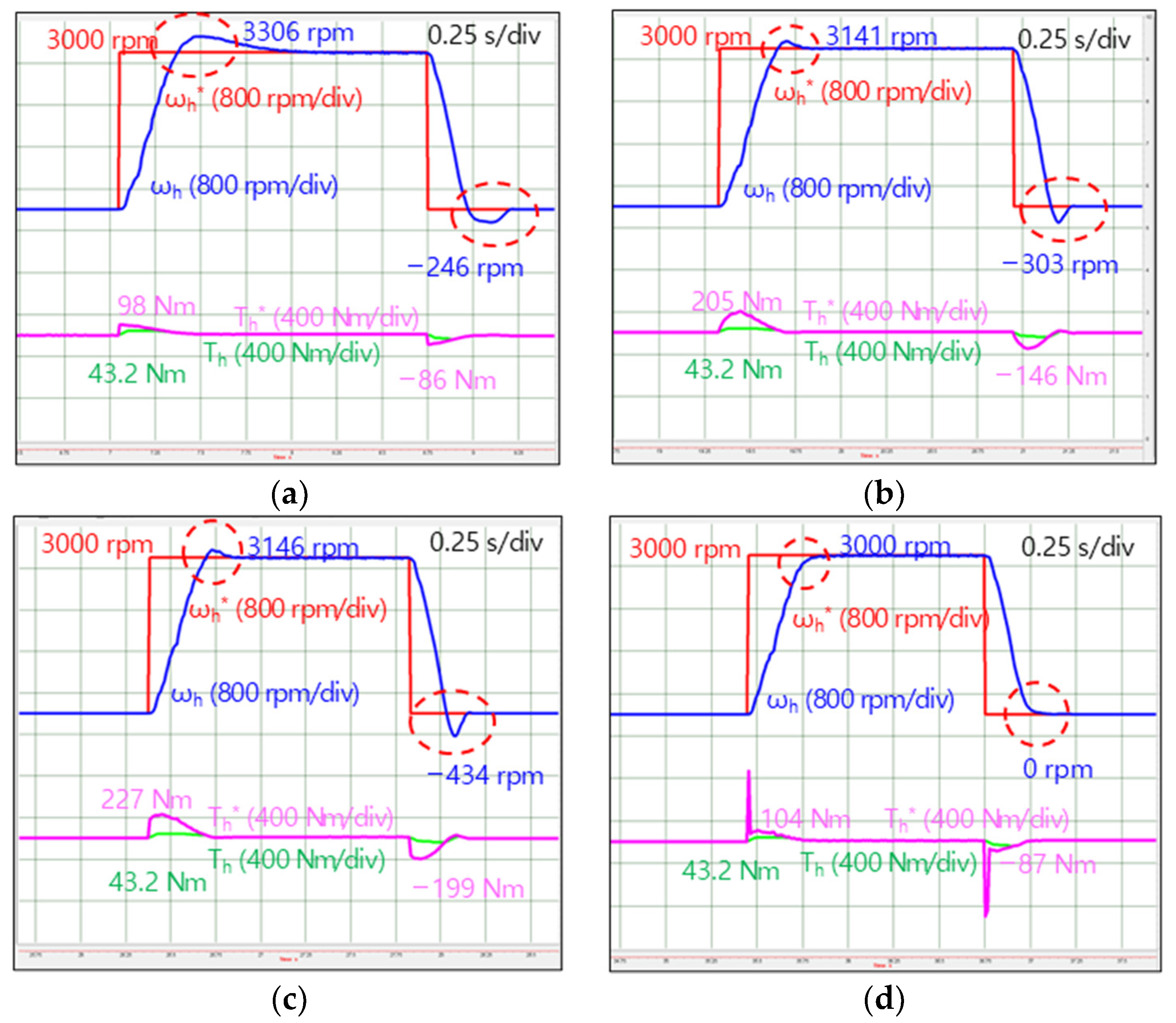
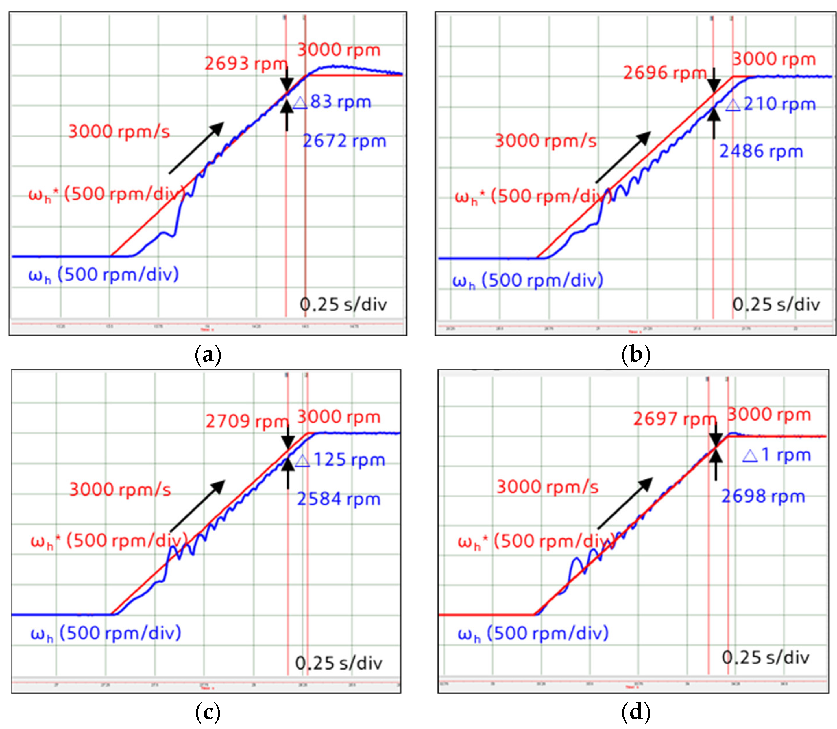
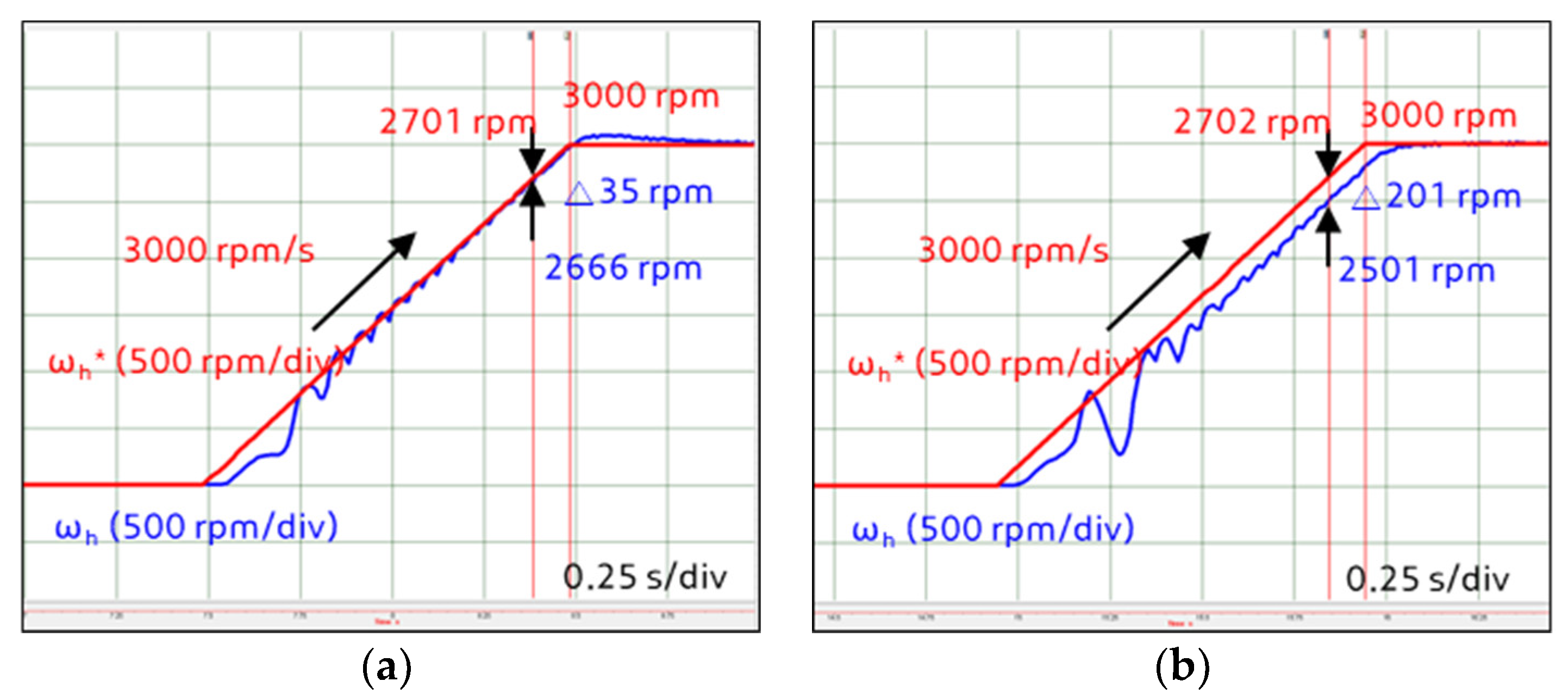
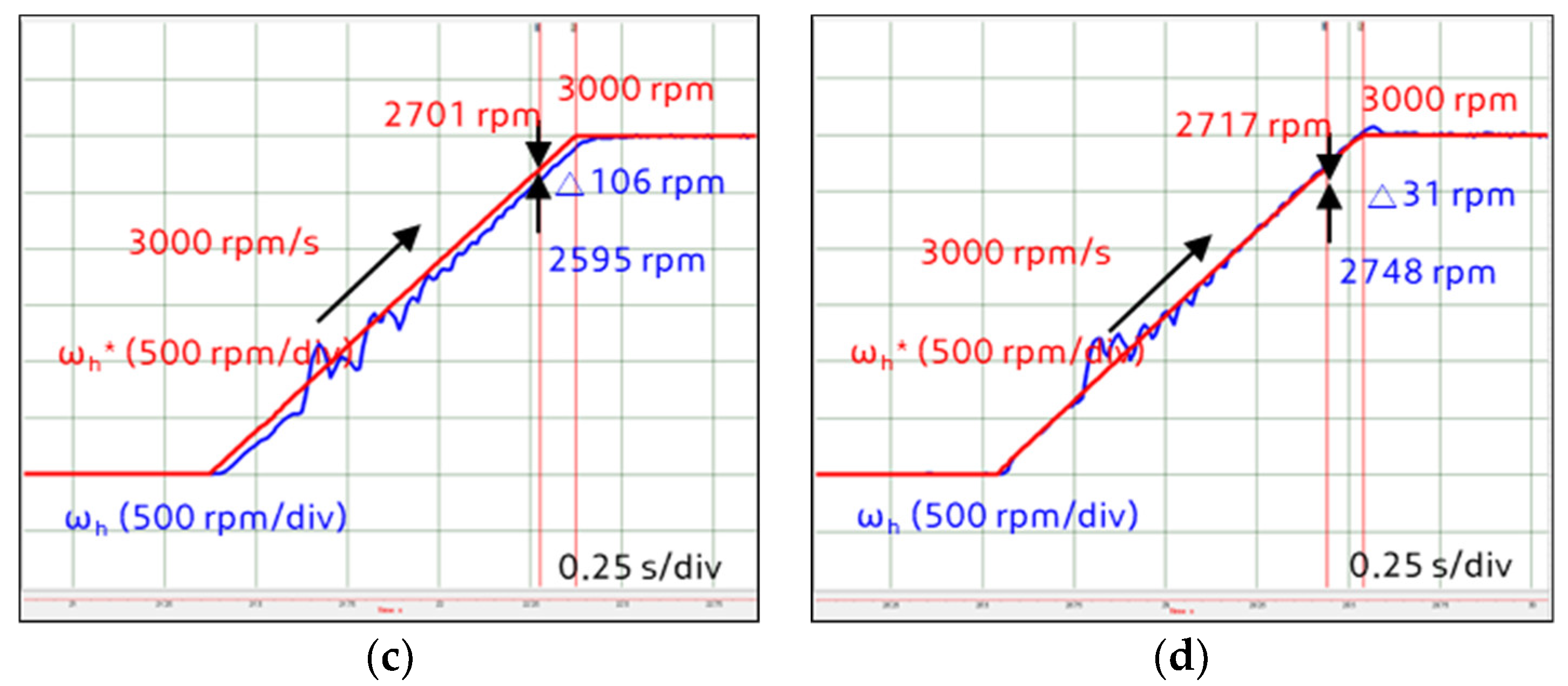
5.1. Step Command Response
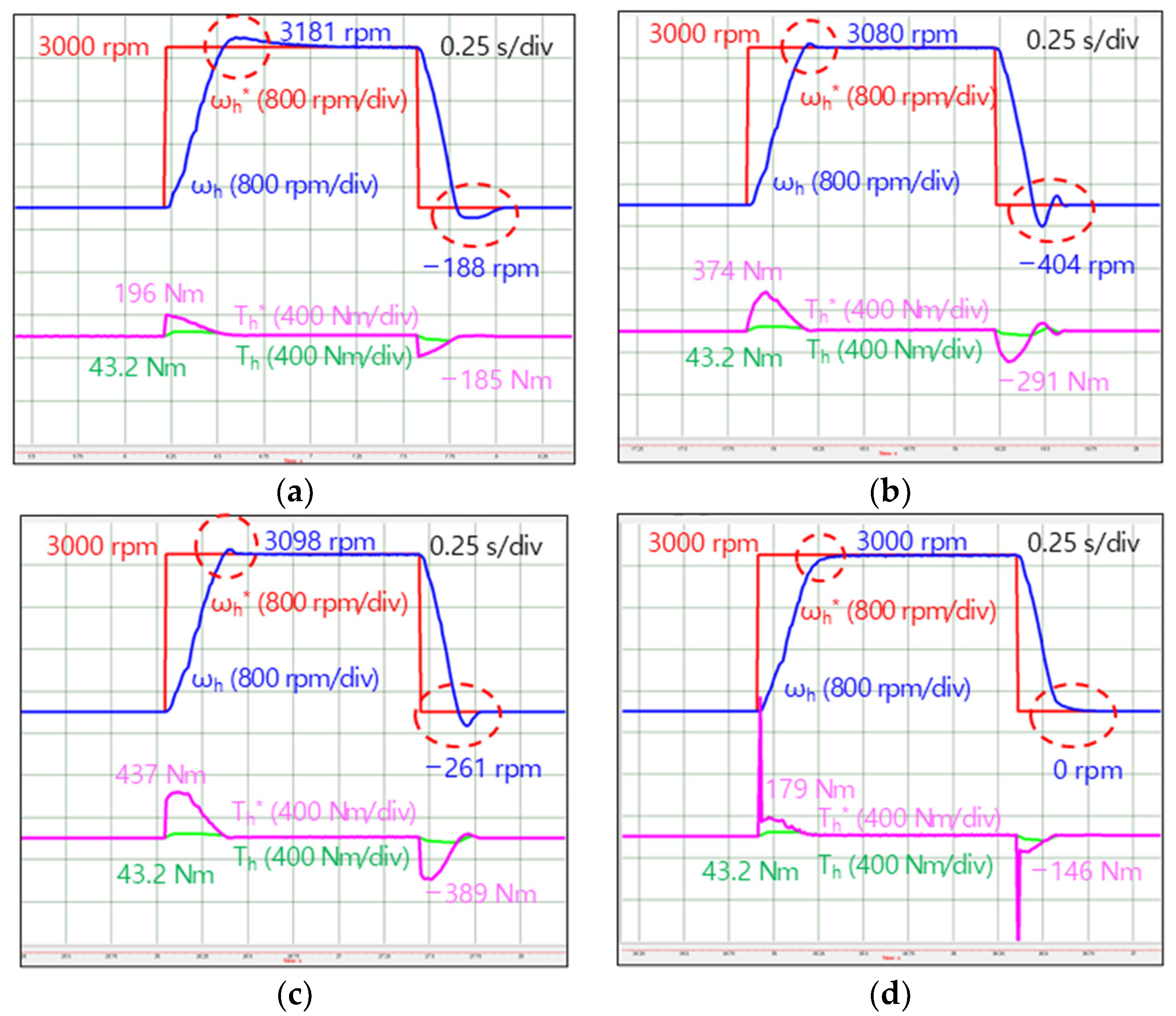
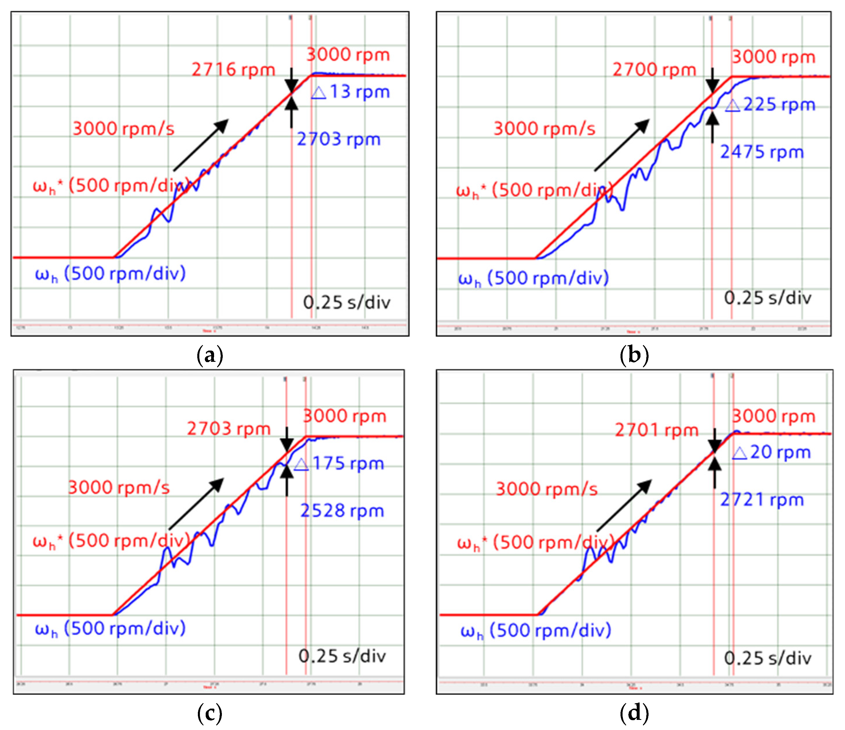
5.2. Ramp Command Response
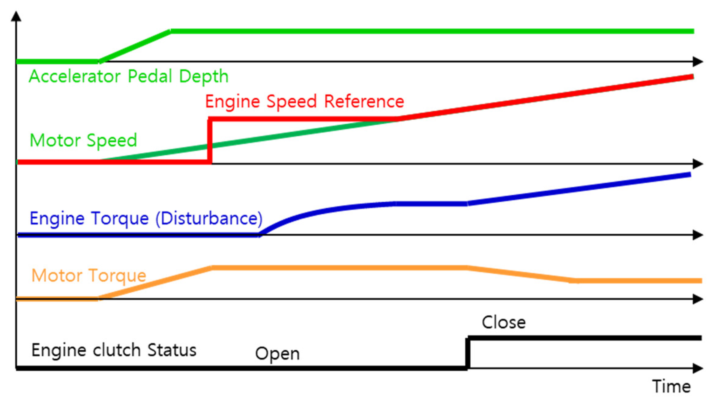
5.3. Vehicle Start Response
6. Conclusions
Author Contributions
Funding
Conflicts of Interest
References
- LaFrance, R.C.; Schult, R.W. Electrical systems for hybrid vehicles. IEEE Trans. Veh. Technol. 1973, 22, 13–19. [Google Scholar] [CrossRef]
- Kim, H.; Wi, J.; Yoo, J.; Son, H.; Kim, H.; Park, C. Influence of Number of Gear Step on Engine and Motor Operation Characteristics for Parallel HEV. In Proceedings of the 2018 Thirteenth International Conference on Ecological Vehicles and Renewable Energies (EVER), Monte-Carlo, Monaco, 10–12 April 2018; pp. 1–7. [Google Scholar]
- Seung-Ki, S. Control of Electric Machine Drive Systems; (in Korean); Hongrung: Seoul, Korea, 2007; pp. 240–245. [Google Scholar]
- Nandam, P.K.; Sen, P.C. Analog and Digital Speed Control of DC Drives Using Proportional-Integral and Integral-Proportional Control Techniques. IEEE Trans. Ind. Electron. 1987, 2, 227–233. [Google Scholar] [CrossRef]
- Umeno, T.; Hori, Y. Robust speed control of DC servomotors using modern two degrees-of-freedom controller design. IEEE Trans. Ind. Electron. 1991, 38, 363–368. [Google Scholar] [CrossRef]
- Li, S.; Liu, Z. Adaptive Speed Control for Permanent-Magnet Synchronous Motor System with Variations of Load Inertia. IEEE Trans. Ind. Electron. 2009, 56, 3050–3059. [Google Scholar]
- Lin, F.J.; Lee, T.S.; Lin, C.H. Robust H∞ controller design with recurrent neural network for linear synchronous motor drive. IEEE Trans. Ind. Electron. 2003, 50, 456–470. [Google Scholar]
- Lai, C.; Shyu, K.-K. A novel motor drive design for incremental motion system via sliding-mode control method. IEEE Trans. Ind. Electron. 2005, 52, 499–507. [Google Scholar] [CrossRef]
- Baik, I.-C.; Kim, K.-H.; Youn, M.-J. Robust nonlinear speed control of PM synchronous motor using boundary layer integral sliding mode control technique. IEEE Trans. Control Syst. Technol. 2000, 8, 47–54. [Google Scholar] [CrossRef]
- Kim, K.-H.; Youn, M.-J. A nonlinear speed control for a PM synchronous motor using a simple disturbance estimation technique. IEEE Trans. Ind. Electron. 2002, 49, 524–535. [Google Scholar]
- Li, S.; Liu, H.; Ding, S. A speed control for a PMSM using finite-time feedback control and disturbance compensation. Trans. Inst. Meas. Control 2010, 32, 170–187. [Google Scholar]
- Li, C.; Chen, M.; Gao, S. Fractional Order PI Speed Control for Permanent Magnet Synchronous Motor Drives. In Proceedings of the 11th World Congress on Intelligent Control and Automation, Shenyang, China, 29 June–4 July 2014; pp. 4681–4685. [Google Scholar]
- Liaw, C.M.; Cheng, S.Y. Fuzzy two-degrees-of-freedom speed controller for motor drives. IEEE Trans. Ind. Electron. 1995, 42, 209–216. [Google Scholar] [CrossRef]
- Zhen, L.; Xu, L. Fuzzy learning enhanced speed control of an indirect field-oriented induction machine drive. IEEE Trans. Control Syst. Technol. 2000, 8, 270–278. [Google Scholar] [CrossRef]
- Kung, Y.S.; Ouyang, M.; Liaw, C.M. Adaptive speed control for induction motor drives using neural networks. IEEE Trans. Ind. Electron. 1995, 42, 25–32. [Google Scholar] [CrossRef]
- Chen, T.-C.; Sheu, T.-T. Model reference neural network controller for induction motor speed control. IEEE Trans. Energy Convers. 2002, 17, 157–163. [Google Scholar] [CrossRef]
- Bang, J.S.; Choi, S.H.; Ko, Y.K.; Kim, T.S.; Kim, S. The Engine Clutch Engagement Control for Hybrid Electric Vehicles. In Proceedings of the 2018 IEEE Conference on Control Technology and Applications (CCTA), Copenhagen, Denmark, 21–24 August 2018; pp. 1448–1453. [Google Scholar]
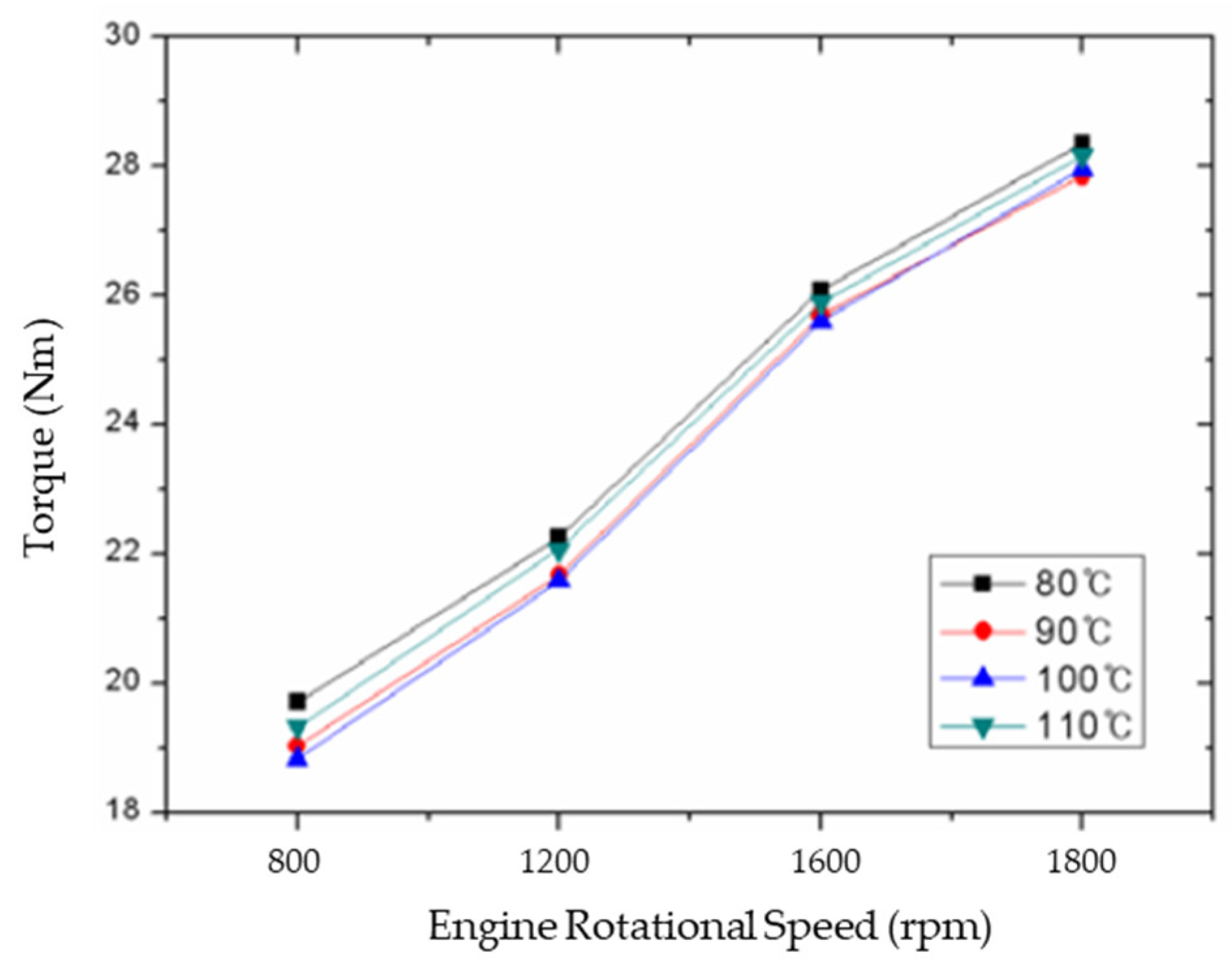
- Kim, H.-I.; Cho, W.; Lee, K. A Fundamental Study of Friction Characteristics According to the Temperature of Engine Oil (in Korean). In Proceedings of the KSAE 2007 Spring Conference, Changwon, Korea, 21–23 June 2007; pp. 69–74. [Google Scholar]
- Kwon, T.-S.; Sul, S.-K.; Nakamura, H.; Tsuruta, K. Identification of the Mechanical Parameters for Servo Drive. In Proceedings of the Conference Record of the 2006 IEEE Industry Applications Conference Forty-First IAS Annual Meeting, Tampa, FL, USA, 8–12 October 2006; pp. 905–910. [Google Scholar]
- Seok, J.-K.; Lee, D.-C. Speed Controller Design Based on Current Controller Dynamics for Industry Servo Applications (in Korean). In Proceedings of the KIPE Conference, Seoul, Korea, 16 November 2002; pp. 465–471. [Google Scholar]
- Cho, Y.; Byen, B.-J.; Lee, H.-S.; Cho, K.Y. A Single-Loop Repetitive Voltage Controller with an Active Damping Control Technique. Energies 2017, 10, 673. [Google Scholar] [CrossRef]
- Valenzuela, M.A.; Lorenz, R.D. Startup and commissioning procedures for electronically line-shafted paper machine drives. IEEE Trans. Ind. Appl. 2002, 38, 966–973. [Google Scholar] [CrossRef]


| Controller | PI | IP | 2-DOF | Proposed |
|---|---|---|---|---|
| Controller | PI | IP | 2-DOF | Proposed |
|---|---|---|---|---|
| - | - | |||
| - | - | 0.5 | - | |
| - | - | - | Multiple of |
| Controller | PI | IP | 2 DOF | Proposed |
|---|---|---|---|---|
| 0.622 | 1.933 | 1.933 | 0.622 | |
| 2.345 | 28.307 | 28.307 | 49.536 | |
| - | - | 0.5 | - | |
| - | - | - | 2.603 |
| Controller | PI | IP | 2-DOF | Proposed |
|---|---|---|---|---|
| Final value theorem of ramp command: | ||||
| Ramp command error (rpm) | Δ46.05 | Δ208.68 | Δ106.24 | 0 |
| Controller | PI | IP | 2-DOF | Proposed |
|---|---|---|---|---|
| Speed overshoot | 160 | 75 | 101 | 0 |
| Speed variation at load disturbance | 304 | 78 | 78 | 75 |
| Steady-state error (At ramp command) | −6 | 209 | 107 | 1 |
| Controller | Parameters Variation | ||
|---|---|---|---|
| 50% | 100% | 250% | |
| PI | 92.11 | 46.05 | 18.42 |
| IP | 212.49 | 208.68 | 206.39 |
| 2 DOF | 110.06 | 106.24 | 103.95 |
| Proposed | 0.00072 | 0 | −0.0043 |
| Parameters Variation | Control Method | ||||
|---|---|---|---|---|---|
| PI | IP | 2-DOF | Proposed | ||
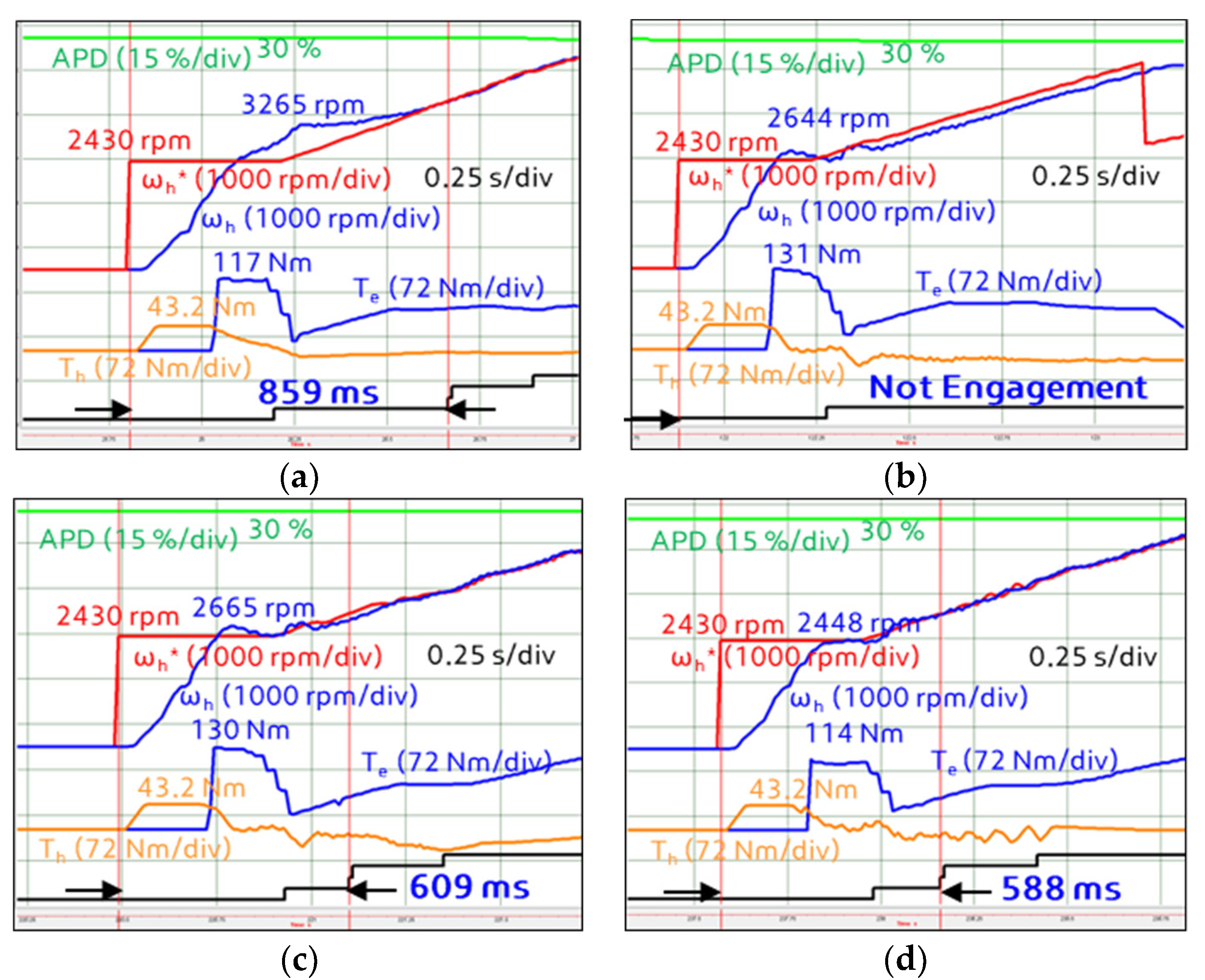
| Engagement Time (ms) | 50% | 859 | - | 609 | 588 |
| Base | - | −29.1% | −31.5% | ||
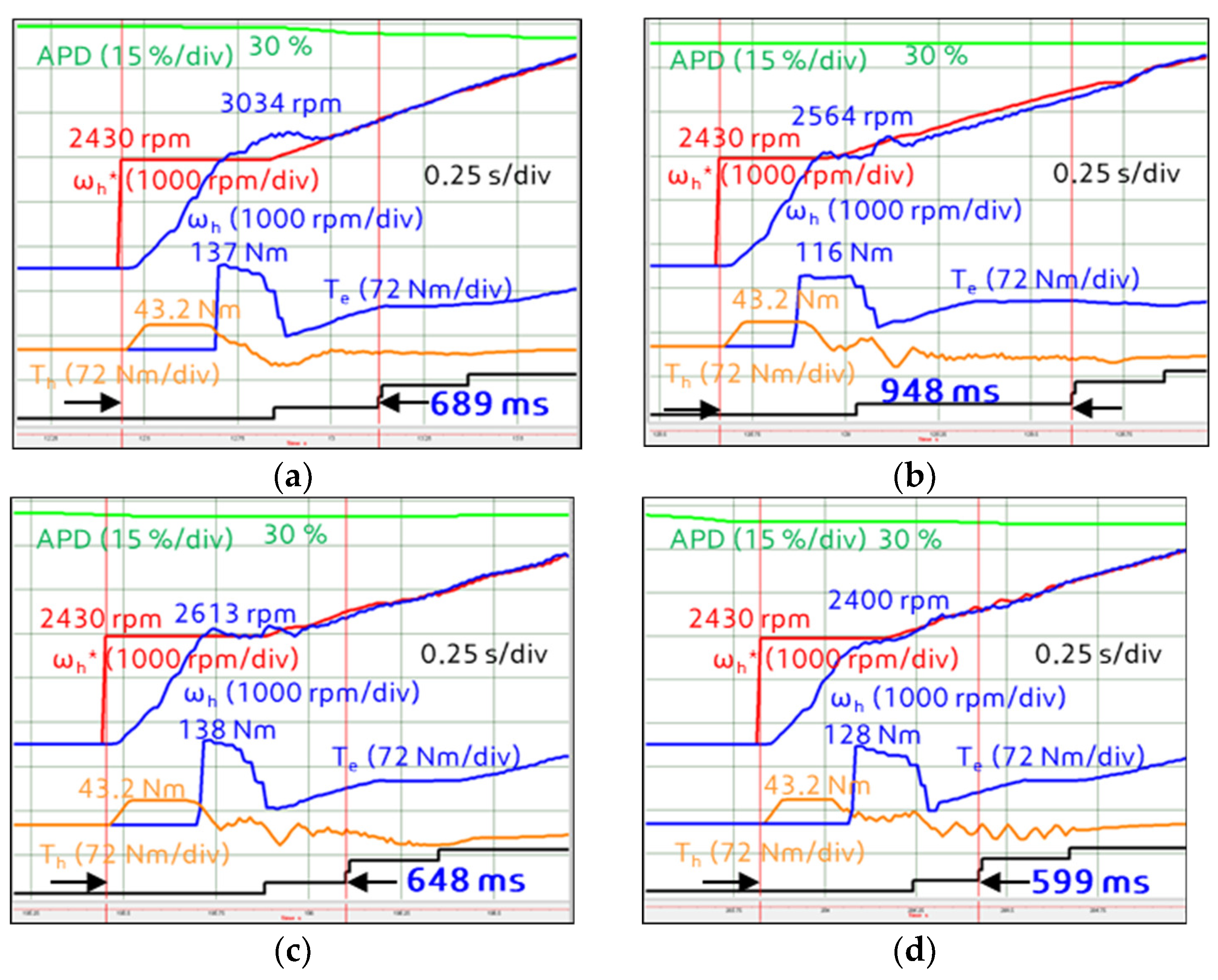
| 100% | 689 | 948 | 648 | 599 | |
| Base | 37.6% | −6.0% | −13.1% | ||
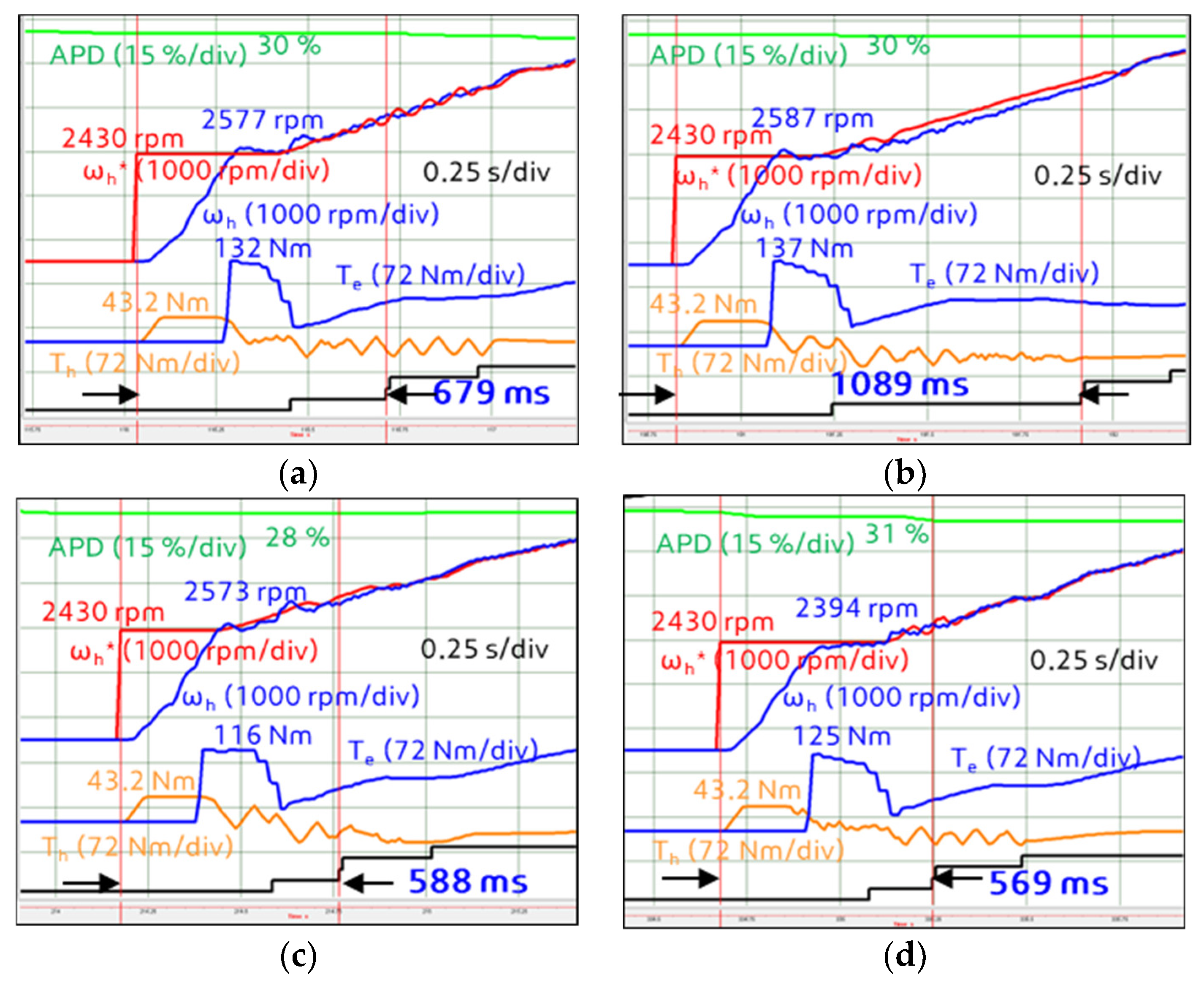
| 250% | 679 | 1089 | 588 | 569 | |
| Base | 58.1% | −14.7% | −17.4% | ||
© 2020 by the authors. Licensee MDPI, Basel, Switzerland. This article is an open access article distributed under the terms and conditions of the Creative Commons Attribution (CC BY) license (http://creativecommons.org/licenses/by/4.0/).
Share and Cite
Yang, B.; Kim, K.; Mok, H. Fast and Robust Hybrid Starter and Generator Speed Control for Improving Drivability of Parallel Hybrid Electric Vehicles. Energies 2020, 13, 5055. https://doi.org/10.3390/en13195055
Yang B, Kim K, Mok H. Fast and Robust Hybrid Starter and Generator Speed Control for Improving Drivability of Parallel Hybrid Electric Vehicles. Energies. 2020; 13(19):5055. https://doi.org/10.3390/en13195055
Chicago/Turabian StyleYang, ByungHoon, KyoungJoo Kim, and HyungSoo Mok. 2020. "Fast and Robust Hybrid Starter and Generator Speed Control for Improving Drivability of Parallel Hybrid Electric Vehicles" Energies 13, no. 19: 5055. https://doi.org/10.3390/en13195055
APA StyleYang, B., Kim, K., & Mok, H. (2020). Fast and Robust Hybrid Starter and Generator Speed Control for Improving Drivability of Parallel Hybrid Electric Vehicles. Energies, 13(19), 5055. https://doi.org/10.3390/en13195055