Author Contributions
Conceptualization, W.H., E.O. and A.D.; methodology, A.D. and E.O.; software, W.H., M.M., E.O.; validation, A.A.; formal analysis, M.N.H. and L.S.; investigation, W.H.; data curation, A.D.; original draft preparation, review and editing, W.H., E.O., A.A., M.B.H., L.F.R. and L.S.; supervision, A.A., M.B.H. and L.S. All authors have read and agreed to the published version of the manuscript.
Figure 1.
Electric scheme of the adopted photovoltaic (PV) system.
Figure 1.
Electric scheme of the adopted photovoltaic (PV) system.
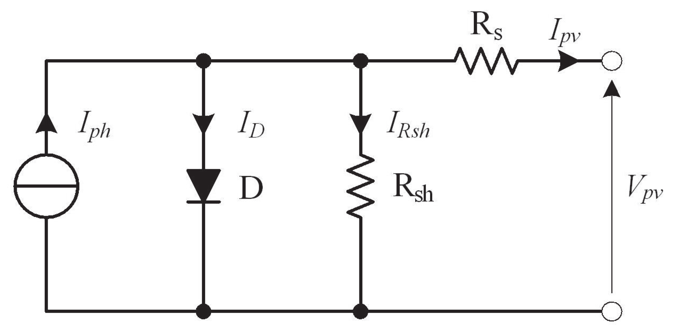
Figure 2.
Five parameter equivalent model of a solar cell.
Figure 2.
Five parameter equivalent model of a solar cell.
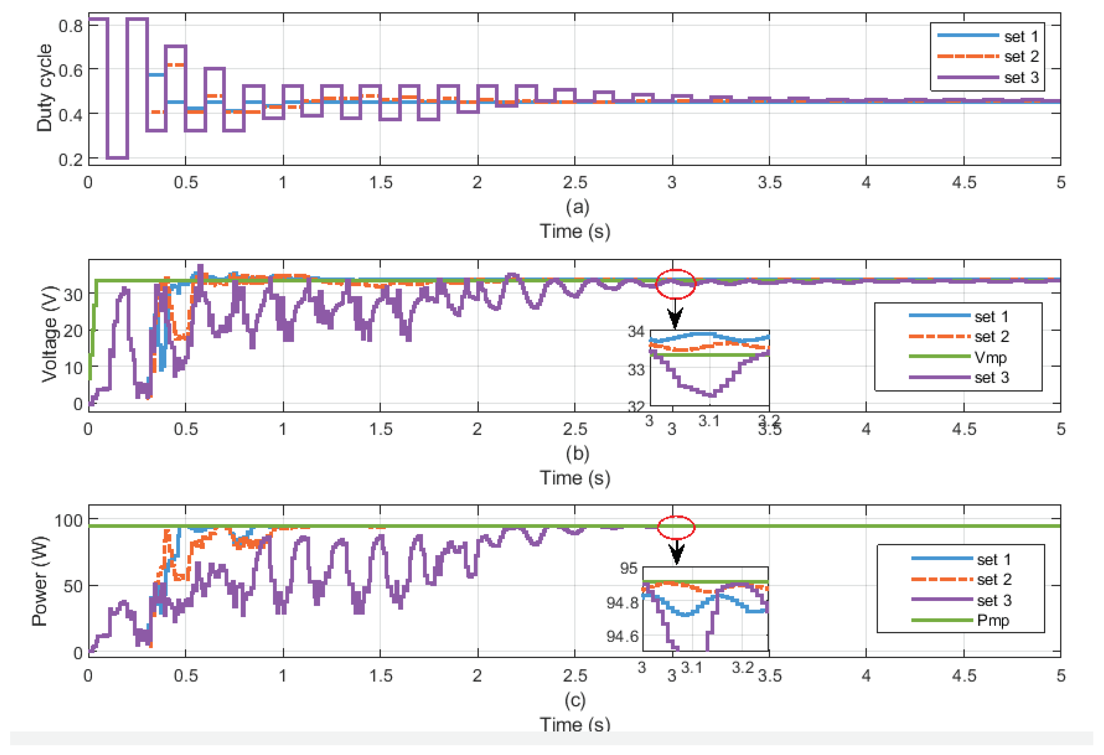
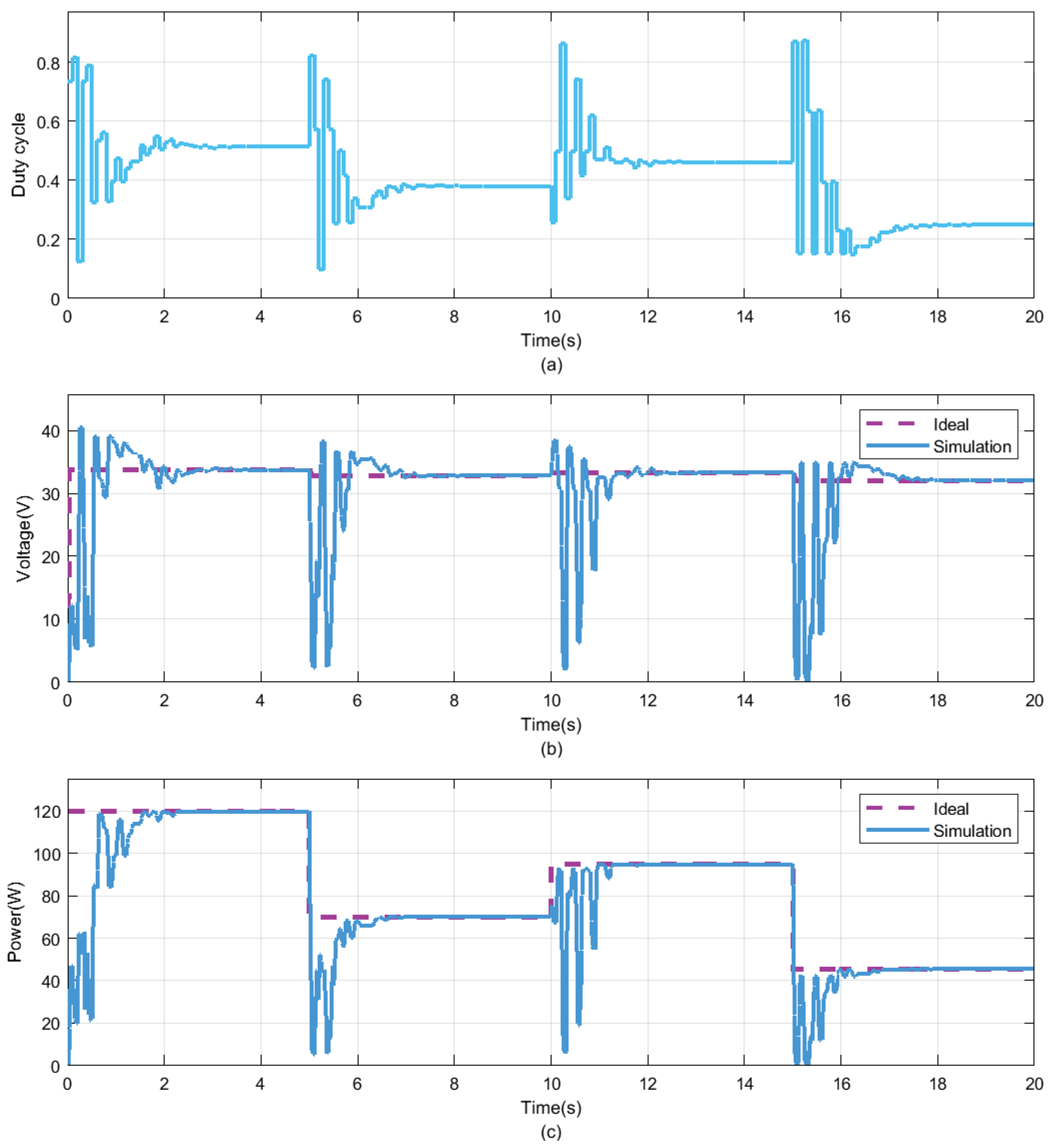
Figure 3.
Simulation results under different sets of parameters w, and given by PSO algorithm at constant irradiance and temperature (G = 800 W/m2, = 25 °C): (a) duty cycle, (b) voltage, and (c) power.
Figure 3.
Simulation results under different sets of parameters w, and given by PSO algorithm at constant irradiance and temperature (G = 800 W/m2, = 25 °C): (a) duty cycle, (b) voltage, and (c) power.
Figure 4.
Flowchart of the Improved Particle Swarm Optimisation (IPSO)-based MPPT algorithm.
Figure 4.
Flowchart of the Improved Particle Swarm Optimisation (IPSO)-based MPPT algorithm.
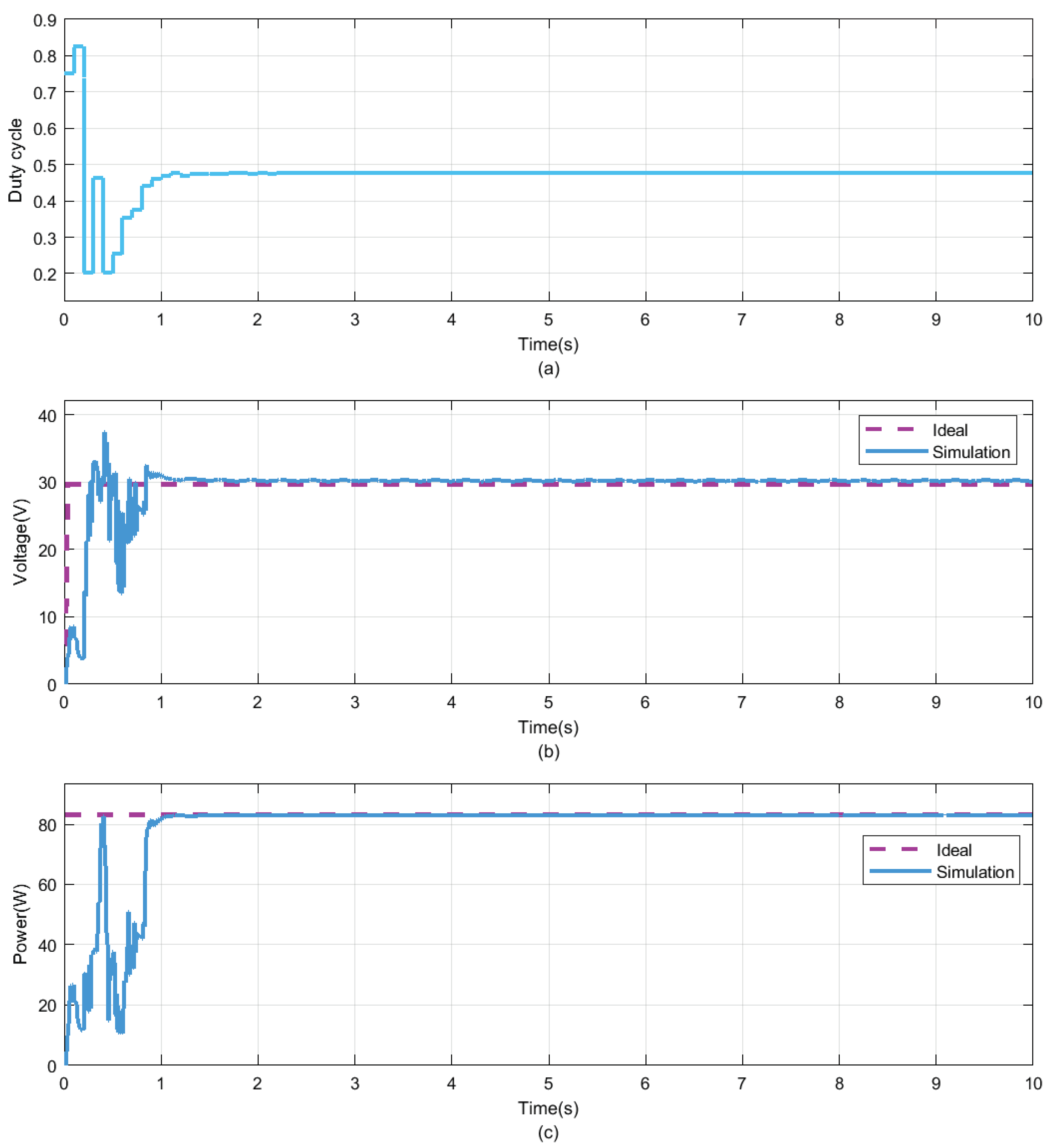
Figure 5.
Simulation results under G = 800 W/m2, = 48 °C and = 2 given by the Improved Particle Swarm Optimisation (IPSO) algorithm: (a) Duty cycle, (b) Voltage, and (c) Power.
Figure 5.
Simulation results under G = 800 W/m2, = 48 °C and = 2 given by the Improved Particle Swarm Optimisation (IPSO) algorithm: (a) Duty cycle, (b) Voltage, and (c) Power.
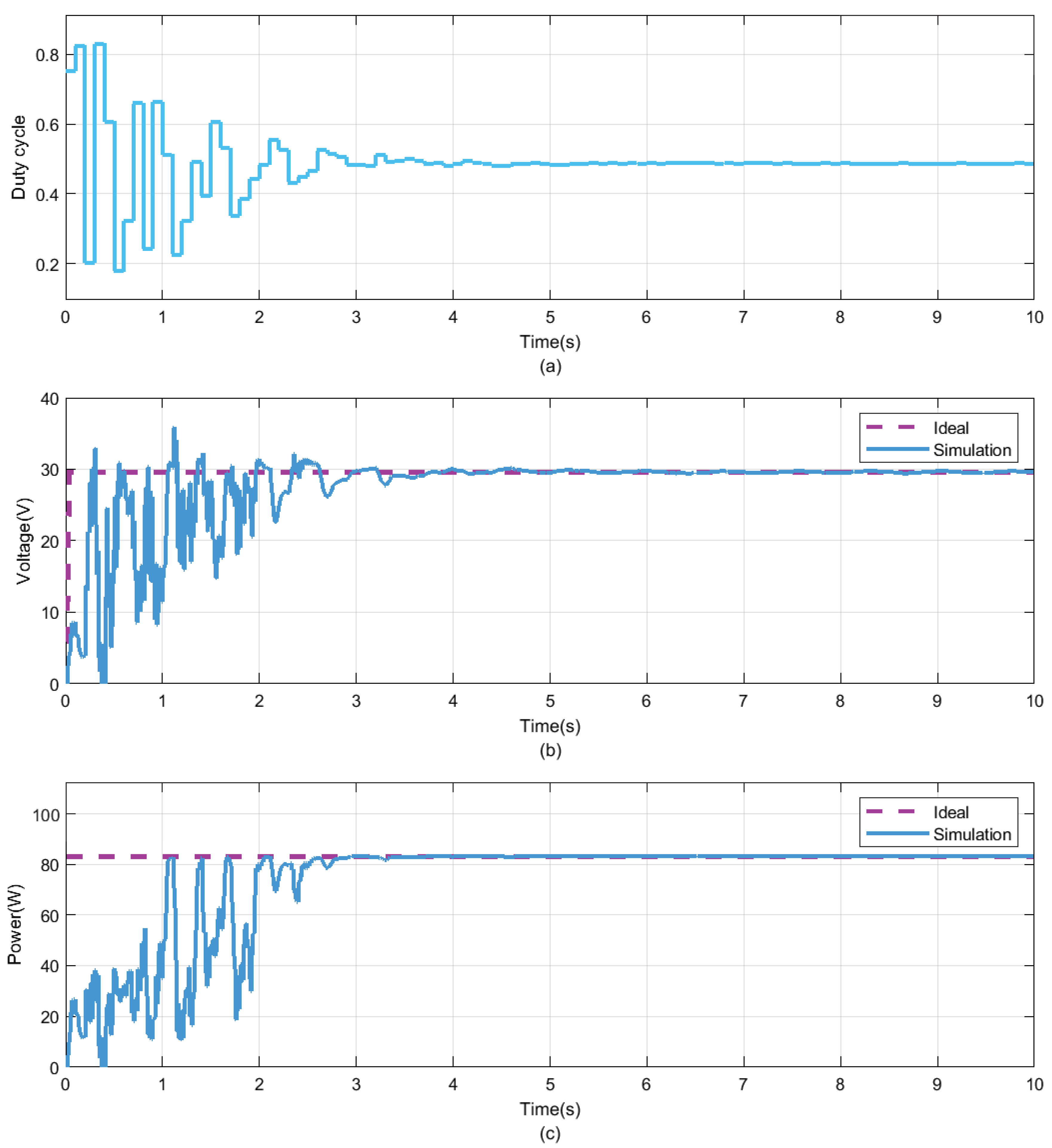
Figure 6.
Simulation results under G = 800 W/m2, = 48 °C and = 3 given by the Improved Particle Swarm Optimisation (IPSO) algorithm: (a) Duty cycle, (b) Voltage, and (c) Power.
Figure 6.
Simulation results under G = 800 W/m2, = 48 °C and = 3 given by the Improved Particle Swarm Optimisation (IPSO) algorithm: (a) Duty cycle, (b) Voltage, and (c) Power.
Figure 7.
Simulation results under G = 800 W/m2, = 48 °C and = 6 given by the Improved Particle Swarm Optimisation (IPSO) algorithm: (a) Duty cycle, (b) Voltage, and (c) Power.
Figure 7.
Simulation results under G = 800 W/m2, = 48 °C and = 6 given by the Improved Particle Swarm Optimisation (IPSO) algorithm: (a) Duty cycle, (b) Voltage, and (c) Power.
Figure 8.
Simulation results under G = 800 W/m2, = 48 °C and = 10 given by the Improved Particle Swarm Optimisation (IPSO) algorithm: (a) Duty cycle, (b) Voltage, and (c) Power.
Figure 8.
Simulation results under G = 800 W/m2, = 48 °C and = 10 given by the Improved Particle Swarm Optimisation (IPSO) algorithm: (a) Duty cycle, (b) Voltage, and (c) Power.
Figure 9.
Irradiance profile of the whole panel without shading.
Figure 9.
Irradiance profile of the whole panel without shading.
Figure 10.
P–V curves of the photovoltaic (PV) panel affected by variable irradiance.
Figure 10.
P–V curves of the photovoltaic (PV) panel affected by variable irradiance.
Figure 11.
Simulation results under irradiance variation and = 2 given by the Improved Particle Swarm Optimisation (IPSO) algorithm: (a) Duty cycle, (b) Voltage under irradiance change, and (c) Power under irradiance change.
Figure 11.
Simulation results under irradiance variation and = 2 given by the Improved Particle Swarm Optimisation (IPSO) algorithm: (a) Duty cycle, (b) Voltage under irradiance change, and (c) Power under irradiance change.
Figure 12.
Simulation results under radiation variation and = 3 given by the Improved Particle Swarm Optimisation (IPSO) algorithm: (a) Duty cycle, (b) Voltage under irradiance change, and (c) Power under irradiance change.
Figure 12.
Simulation results under radiation variation and = 3 given by the Improved Particle Swarm Optimisation (IPSO) algorithm: (a) Duty cycle, (b) Voltage under irradiance change, and (c) Power under irradiance change.
Figure 13.
Shadow affecting of the adopted panel area.
Figure 13.
Shadow affecting of the adopted panel area.
Figure 14.
irradiance values affecting 75% of the panel.
Figure 14.
irradiance values affecting 75% of the panel.
Figure 15.
P–V characteristics in different sets of partially shading.
Figure 15.
P–V characteristics in different sets of partially shading.
Figure 16.
Simulation results under different sets of partially shading and = 2 given by the Improved Particle Swarm Optimization (IPSO) method: (a) Duty cycle, (b) Voltage, and (c) Power.
Figure 16.
Simulation results under different sets of partially shading and = 2 given by the Improved Particle Swarm Optimization (IPSO) method: (a) Duty cycle, (b) Voltage, and (c) Power.
Figure 17.
Simulation results under different sets of partially shading and = 3 given by Improved Particle Swarm Optimization (IPSO) algorithm: (a) Duty cycle, (b) Voltage, and (c) Power.
Figure 17.
Simulation results under different sets of partially shading and = 3 given by Improved Particle Swarm Optimization (IPSO) algorithm: (a) Duty cycle, (b) Voltage, and (c) Power.
Table 1.
BP MSX-120 datasheet parameters.
Table 1.
BP MSX-120 datasheet parameters.
| Maximum power | | 120 W |
| Voltage at | | 33.7 V |
| Current at | | 3.56 A |
| Short circuit | | 3.87 A |
| Open circuit | | 42.1 V |
| Temperature coefficient of | | 0.065 %/°C |
| Temperature coefficient of | | −80 mV/ °C |
Table 2.
BPMSX-120 parameters.
Table 2.
BPMSX-120 parameters.
| Light-generated | | 3.8713 A |
| Diode saturation | | 322.71 nA |
| Diode ideality | n | 1.3976 |
| Series resistance | | 0.4728 |
| Shunt resistance | | 1365.8 |
Table 3.
Parameter values in different sets.
Table 3.
Parameter values in different sets.
| Set | w | | |
|---|
| 1 | 0.2 | 0.2 | 0.6 |
| 2 | 0.34 | 0.33 | 0.33 |
| 3 | 0.2 | 0.6 | 0.2 |
Table 4.
Comparison performances under different PSO parameters.
Table 4.
Comparison performances under different PSO parameters.
| Set | Duty Cycle in the Steady State | (V) | (W) | (%) | Transient Response (s) | |
|---|
| 1 | 0.4508 | 33.6157 | 94.8639 | 6.70 | 0.9 | 99.95 |
| 2 | 0.4705 | 33.4519 | 94.9001 | 7.56 | 1.18 | 99.99 |
| 3 | 0.4514 | 33.3964 | 94.9020 | 19.19 | 3.81 | 99.99 |
Table 5.
Comparison performances under different values.
Table 5.
Comparison performances under different values.
| Duty Cycle in the Steady State | (V) | (W) | (%) | Transient Response (s) | |
|---|
| 2 | 0.4759 | 30.0953 | 83.0623 | 10.75 | 1.77 | 99.84 |
| 3 | 0.4810 | 29.9190 | 83.1429 | 16.76 | 1.5 | 99.94 |
| 6 | 0.4869 | 29.6063 | 83.1905 | 22.60 | 2.97 | 99.99 |
| 10 | 0.4858 | 29.4027 | 83.1705 | 40.96 | 6.58 | 99.97 |
Table 6.
MPPs for photovoltaic (PV) generator under different irradiance at 25 °C.
Table 6.
MPPs for photovoltaic (PV) generator under different irradiance at 25 °C.
| Set | Irradiance (W/m2) | | |
|---|
| P | 1000 | 33.70 | 119.9720 |
| Q | 600 | 32.79 | 69.9888 |
| R | 800 | 33.33 | 94.90 |
| S | 400 | 31.94 | 45.3924 |
Table 7.
Comparison performances of the proposed the Improved Particle Swarm Optimisation (IPSO) method when = 2 and = 3.
Table 7.
Comparison performances of the proposed the Improved Particle Swarm Optimisation (IPSO) method when = 2 and = 3.
| Set | Duty Cycle | (V) | (W) | (%) | Transient Duration (s) | (%) |
|---|
| = 2 | P | 0.5115 | 33.8109 | 119.9635 | 4.78 | 2.26 | 99.9929 |
| | Q | 0.3939 | 32.0184 | 69.7521 | 4.63 | 2.86 | 99.6618 |
| | R | 0.4589 | 33.3224 | 94.9072 | 2.42 | 1.85 | 99.9998 |
| | S | 0.2475 | 31.8400 | 45.3885 | 2.25 | 1.66 | 99.9914 |
| = 3 | P | 0.5132 | 33.7030 | 119.9720 | 9.79 | 3.46 | 100 |
| | Q | 0.3795 | 32.7413 | 69.9874 | 7.15 | 2.36 | 99.9979 |
| | R | 0.4593 | 33.3393 | 94.9073 | 5.42 | 3.06 | 100 |
| | S | 0.2474 | 32.0115 | 45.3915 | 8.72 | 3.26 | 99.9980 |
Table 8.
Comparison accuracy between the Improved Particle Swarm Optimisation (IPSO), Neural Network (NN)-Particle Swarm Optimisation (PSO) [
30], and PSO-Perturb & Observe (P&O) [
31].
Table 8.
Comparison accuracy between the Improved Particle Swarm Optimisation (IPSO), Neural Network (NN)-Particle Swarm Optimisation (PSO) [
30], and PSO-Perturb & Observe (P&O) [
31].
| Algorithm | Set | (W) | (W) | (%) |
|---|
| ANN-PSO [30] | P | 669.1 | 897.3 | 74.57 |
| | Q | 665.7 | 723.2 | 92.05 |
| | R | 439.3 | 544.7 | 80.65 |
| | S | 302.1 | 362.5 | 83.34 |
| PSO-P&O [31] | P | 99.5 | 100.7 | 98.81 |
| | Q | 58.71 | 59.8 | 98.18 |
| | R | 79.42 | 80.7 | 98.41 |
| | S | - | - | - |
| IPSO ( = 3) | P | 119.9720 | 119.9720 | 100 |
| | Q | 69.9874 | 69.9888 | 99.9979 |
| | R | 94.9073 | 94.9073 | 100 |
| | S | 45.3915 | 45.3924 | 99.9980 |
Table 9.
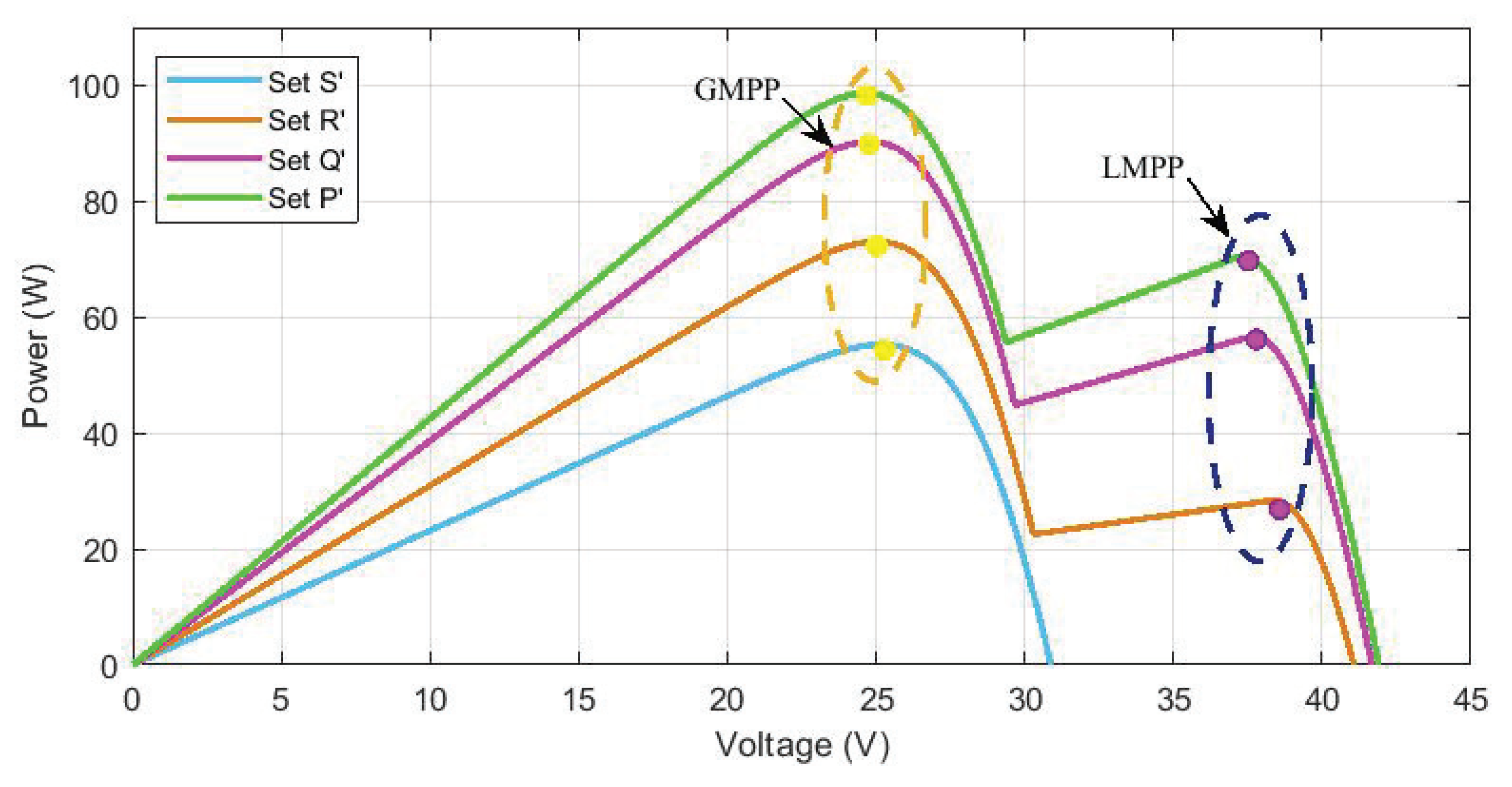
Global MPP (GMPP) and local MPP (LMPP) for photovoltaic (PV)generator under different sets of partial shading at 25 °C.
Table 9.
Global MPP (GMPP) and local MPP (LMPP) for photovoltaic (PV)generator under different sets of partial shading at 25 °C.
| Set | Time (s) | G (W/m2) | SI (%) | GS (W/m2) | GMPP | LMPP |
|---|
| | | | | | | | | |
| P’ | [0,5] | 1000 | 40 | 600 | 25.18 | 90.2943 | 37.75 | 56.89 |
| Q’ | [5,10] | 600 | 0 | 600 | 25.18 | 55.2495 | 25.18 | 55.24 |
| R’ | [10,15] | 800 | 25 | 600 | 25 | 73.0760 | 38.48 | 28.5 |
| S’ | [15,20] | 1100 | 45.46 | 600 | 24.63 | 98.6604 | 37.36 | 70.69 |
Table 10.
Performance comparison of Improved Particle Swarm Optimization (IPSO) method under partial shading when = 2 and = 3.
Table 10.
Performance comparison of Improved Particle Swarm Optimization (IPSO) method under partial shading when = 2 and = 3.
| Set | Duty Cycle | (V) | (W) | (%) | Transient Duration (s) |
|---|
| 2 | P’ | 0.5310 | 26.9670 | 82.6659 | 13.47 | 3.56 |
| | Q’ | 0.4773 | 24.5042 | 54.9416 | 4.92 | 2.56 |
| | R’ | 0.5310 | 25.3353 | 72.9674 | 4.12 | 2.66 |
| | S’ | 0.6081 | 24.6476 | 98.6605 | 3.38 | 1.96 |
| 3 | P’ | 0.5886 | 24.7296 | 90.2913 | 12.97 | 3.96 |
| | Q’ | 0.4658 | 25.1612 | 55.2495 | 9.89 | 3.26 |
| | R’ | 0.5380 | 25.0289 | 73.0759 | 6.43 | 3.26 |
| | S’ | 0.6071 | 24.5797 | 98.6555 | 8.33 | 3.66 |
Table 11.
Accuracy comparison between techniques (Improved Particle Swarm Optimization (IPSO)) and (Particle Swarm Optimization (PSO), Genetic Algorithm(GA)) methods under partial shading.
Table 11.
Accuracy comparison between techniques (Improved Particle Swarm Optimization (IPSO)) and (Particle Swarm Optimization (PSO), Genetic Algorithm(GA)) methods under partial shading.
| Algorithm | Set | (W) | PGMPP (W) | (%) |
|---|
| PSO [32] | P’ | 237.5 | 239 | 99.4 |
| | Q’ | 249.9 | 255.8 | 97.7 |
| | R’ | 257.2 | 261.2 | 98.5 |
| | S’ | 255.7 | 263.7 | 97 |
| GA [32] | P’ | 230.8 | 239 | 96.6 |
| | Q’ | 244.5 | 255.8 | 95.6 |
| | R’ | 247 | 261.2 | 94.6 |
| | S’ | 248.9 | 263.7 | 94.4 |
| IPSO ( = 3) | P’ | 90.2913 | 90.2943 | 99.99 |
| | Q’ | 55.2495 | 55.2495 | 100 |
| | R’ | 73.0759 | 73.0760 | 99.99 |
| | S’ | 98.6555 | 98.6604 | 99.99 |

 ,
, 


