Abstract
The sixth-generation (6G) mobile networks are expected to operate at a higher frequency to achieve a wider bandwidth and to enhance the frequency reuse efficiency for improved spectrum utilization. In this regard, three-dimensional (3D) spatial reuse of millimeter-wave (mmWave) spectra by in-building small cells is considered an effective technique. In contrast to previous works exploiting microwave spectra, in this paper, we present a technique for the 3D spatial reuse of 28 and 60 GHz mmWave spectra by in-building small cells, each enabled with dual transceivers operating at 28 and 60 GHz bands, to enhance frequency reuse efficiency and achieve the expected spectral efficiency (SE) and energy efficiency (EE) requirements for 6G mobile networks. In doing so, we first present an analytical model for the 28 GHz mmWave spectrum to characterize co-channel interference (CCI) and deduce a minimum distance between co-channel small cells at both intra- and inter-floor levels in a multistory building. Using minimum distances at both intra- and inter-floor levels, we find the optimal 3D cluster size for small cells and define the corresponding 3D spatial reuse factor, such that the entire 28 and 60 GHz spectra can be reused by each 3D cluster in each building. Considering a system architecture where outdoor macrocells and picocells operate in the 2 GHz microwave spectrum, we derive system-level average capacity, SE, and EE values, as well as develop an algorithm for the proposed technique. With extensive numerical and simulation results, we show the impacts of 3D spatial reuse of multi-mmWave spectra by small cells in each building and the number of buildings per macrocell on the average SE and EE performances. Finally, it is shown that the proposed technique can satisfy the expected average SE and EE requirements for 6G mobile networks.
1. Introduction
Given that fifth-generation (5G) mobile communication networks are scheduled to be commercially deployed in 2020, researchers are looking forward to the next-generation (i.e., sixth-generation (6G)) mobile communication networks. In line with this, both academics and industry researchers have started discussing the structure of 6G, while several proposals for 6G vision and enabling techniques have already been recommended [1,2,3,4]. Because of the highly diversified nature of these proposals, it is very hard to compile a definite set of requirements and enabling techniques at this moment. However, there is a common expectation regarding the 10-fold improved performance of 6G over its predecessor 5G networks in terms of several key performance metrics, including average user data rate, system capacity, spectral efficiency, and energy efficiency. Since most data is generated in indoor environments, particularly in urban multistory buildings, developing new techniques to utilize spectra in the high-frequency bands (including millimeter-wave (mmWave), terahertz, and visible light bands) to address high user data rate, system capacity, spectral efficiency (SE), and energy efficiency (EE) demands for the future 6G mobile networks has been proposed as one of the key pillars [1,3,4].
Spatial spectrum reuse techniques have been considered as effective techniques to improve spectrum utilization. However, traditional approaches to spectrum reuse by base stations in two-dimensional (2D) space are not sufficient to address the envisaged user data rate, system capacity, SE, and EE demands of 6G mobile networks. High-frequency bands are coverage-limited due to associated high propagation loss. Moreover, the penetration losses of high-frequency mmWave bands through external and internal walls and floors in any multistory building are significant compared to low-frequency microwave bands. For these reasons, the reuse of high-frequency mmWave bands are explored in the third dimension (i.e., the height of a multistory building), which results in reusing the same high-frequency band more than once at the inter-floor level. In addition, the conventional spectrum reuse techniques at the intra-floor level in a multistory building are used in order to facilitate extensive reuse of mmWave spectra in ultra-dense deployed small cells within the building.
Importantly, the capacity is directly proportional to the available spectrum bandwidth of a channel, which can be extended by increasing either the number of available spectra, such that each small cell can operate in more than one spectrum; or the number of times the same spectrum is reused by small cells through vertical spatial reuse in a multistory building. Hence, techniques for three-dimensional (3D) spatial reuse of high-frequency mmWave spectra with in-building multiband-enabled small cells can achieve the predicted 10-fold increase of the average user data rate, system capacity, SE, and EE of 5G systems to address the expected requirements of the future 6G mobile networks.
Applying a multiband cooperative network architecture for 5G heterogeneous networks is mandatory to address seamless coverage [5]. Moreover, numerous studies on multiband-enabled network architectures have been carried out in the literature. The authors of [5] proposed a control/user plane split-based multiband cooperative network architecture where small access points are considered, enabling multiple mmWave bands to serve user plane data and high data rate demands, while macrocells are enabled with sub-6GHz bands to serve control plane signals and to enable coverage for 5G heterogeneous networks. Likewise, an architecture for long-term evolution (LTE) systems considering unlicensed bands for splitting control and user plane data is proposed in [6], the fundamentals and general structure of a control and user plane split architecture are proposed in [7], and a mobility management scheme for ultra-dense networks is proposed in [8].
However, studies on multiband-enabled in-building small cells used to exploit the vertical spatial reuse of spectra are not obvious. We first studied this case and proposed techniques to show the potential to achieve high spectral and energy efficiencies in both fourth generation (4G) [9] and 5G [10,11,12] networks by exploiting both microwave and mmWave spectrum sharing with small cells of the same or a different system. This paper extends the contribution of these previous studies, where small cells are enabled only with high-frequency bands, by reusing these spectrum bands as much as possible with each small cell to address the expected requirements for 6G. Unlike previous works, multi-millimeter-wave (multi-mmWave) channel models are exploited to define a more accurate 3D cluster of small cells to reuse the whole spectrum with each cluster of small cells. Since the microwave spectrum is not reused by small cells and because 28 and 60 GHz mmWave spectra of the mobile network operator (MNO) are reused only by in-building small cells, no co-channel interference management technique is needed, unlike in previous studies. Transceiver 1 for each small cell operates in the 28 GHz licensed spectrum band, whereas transceiver 2 operates in the 60 GHz unlicensed spectrum band.
Based on the service requirements, both intra-floor- and inter-floor-level co-channel interference constraints are set to define a minimum distance between co-channel interferers at both intra-floor and inter-floor levels, which in turns gives the size of a 3D cluster of small cells. The entire 28 and 60 GHz spectra are reused by each 3D cluster in each building for L number of buildings where L denotes the number of buildings of small cells per macrocell. The average system-level capacity, SE, and EE performance metrics are derived for numerous values of 3D spatial reuse factors. Finally, the performance of the proposed technique is then compared with that of 6G mobile networks to show that the 3D spatial reuse of multi-mmWave spectra can satisfy the average SE and EE requirements for 6G mobile networks.
The paper is organized as follows. The system model, including the system architecture and modeling of 3D clusters of in-building small cells operating in multi-mmWave spectrum bands, is detailed in Section 2. In Section 3, system-level average capacity, SE, and EE performance metrics are derived and an algorithm for the proposed technique for 3D in-building spatial reuse of multi-mmWave spectra in ultra-dense small cells are developed. Performance evaluation, as well as performance comparison of the proposed technique with the expected requirements for 6G in terms of average SE and EE, is carried out in Section 4. We conclude the paper in Section 5.
2. System Model
2.1. System Architecture
First, we consider a system architecture of an MNO, as shown in Figure 1, which incorporates a set of picocells and small cells distributed over the coverage of a macrocell. Picocells serve outdoor users, particularly in hotspot areas, by offloading users from the macrocell. All outdoor macro user equipment (UE) is served either by the macrocell or by a picocell if offloaded. However, if a macro UE is found within a building, the corresponding indoor macro UE is served only by the macrocell. Small cells are deployed only within multistory buildings, such that in-building small cell UE is served only by small cells.
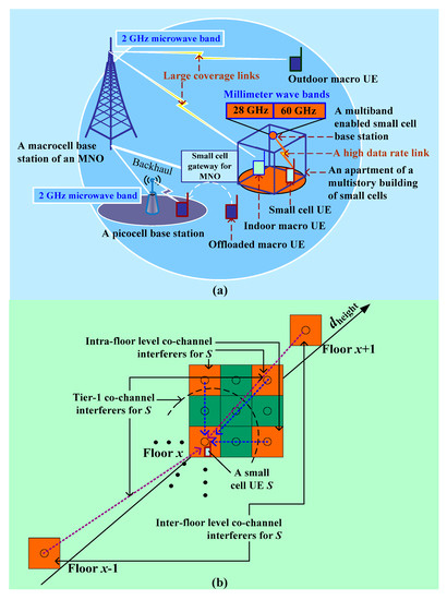
Figure 1.
(a) An illustration of the system architecture for reuse of millimeter-wave (mmWave) spectra for in-building small cells. (b) Co-channel interferers with both intra-floor and inter-floor levels for small-cell user equipment (UE).
Assume that the MNO is allocated with the licensed and 28 GHz spectrum bands to operate 5G mobile networks. To increase the available spectrum bandwidth, assume that the MNO also considers operating at the 60 GHz unlicensed spectrum band. Due to the good channel quality and to ensure extensive coverage, we assume that macrocells operate only in the 2 GHz microwave spectrum, whereas to provide high data rate services within small coverage areas, small cells operate in both mmWave spectra, such that each small cell is enabled with dual-band operation in 28 and 60 GHz bands, as shown in Figure 1a.
Similar to [9], we assume that each building consists of a set of square grid apartments measuring 10 × 10 m2 per floor, and that there are multiple floors per building. For simplicity, we assume that each building has the same number of small cells, although in practice the number of apartments per building varies. Further, we assume that each small cell serves only one UE at any time and is located at the center of the ceiling of an apartment, as shown in Figure 1b. It is to be noted that since macrocells and small cells operate at different frequencies, and that all macro UE and small cell UE are served only by their respective cells, no co-channel interference management technique is needed between macrocell UE and small-cell UE. However, the reuse of the same mmWave spectra is considered within small cells in each building by forming a set of three-dimensional clusters of small cells that satisfy an optimal value of co-channel interference for any small-cell UE. Figure 1b shows the formation of a 3D cluster of small cells for any small-cell UE S within a building, satisfying an optimal co-channel interference value set by the MNO for both intra-floor and inter-floor levels, which we discuss in more detail in the following section.
2.2. Modeling 3D Clusters of Millimeter-Wave Multiband Small Cells
2.2.1. Floor Attenuation Loss
Even though indoor radio signal propagation modeling has been studied for a long time, no standard methodology has yet been developed to measure the penetration loss of walls and floors for different building materials, making it difficult to compare results [13]. Moreover, studies at high frequencies are also limited in the literature, particularly in millimeter frequency bands. Hence, following [14], we consider a typical reinforced concrete floor for modeling purposes. According to [14], the penetration loss of a typical reinforced concrete floor with a suspended false ceiling is 20 dB at 5.2 GHz. Since the floor penetration loss is frequency-dependent and increases rapidly with an increase in frequency, using the floor penetration loss data at 24 GHz in [15] and fitting the curve for a concrete block in [13], we assume that the floor penetration loss in the 28 GHz mmWave spectrum is 55 dB for the first floor as a worst case analysis. Note that the floor penetration loss is not fixed for all floors between transmitters and receivers. Instead, the impact of floor penetration loss is nonlinear, whereby it decreases with an increase in the number of floors.
Moreover, according to [16], an internal wall exhibits a penetration loss of 6.84 dB at 28 GHz. Furthermore, outdoor external tinted glass causes 40.1 dB penetration loss, whereas brick walls show penetration loss of 28 dB at 28 GHz (Table 1). This large penetration loss at 28 GHz for both intra-floor and inter-floor levels, along with high external wall penetration loss, causes the radio frequency to be confined within a building, resulting in no or insignificant interference with outdoor signals of the same frequency. Due to the higher frequency, the loss also increases at 60 GHz as compared to 28 GHz, such that the 3D cluster model of small-cell base stations (SBSs) with the 28 GHz spectrum is also applicable for the 60 GHz unlicensed spectrum.

Table 1.
Floor penetration loss in the 28 GHz mmWave spectrum band.
2.2.2. Modeling of 28 GHz Interference
To model 28 GHz mmWave path loss, we consider the omnidirectional, multi-frequency, combined polarization, close-in free space (CIF) reference distance with the large-scale, frequency-dependent path loss exponent model, as given below.
where n denotes the path loss exponent, b represents the slope of the linear frequency dependence of the path loss, f0 represents a fixed reference frequency serving as the balancing point of the linear frequency dependence of n, and is the Gaussian random variable, with standard deviation representing large-scale signal variation about the mean path loss due to shadowing.
For line-of-sight (LOS) cases, n = 2.1, b = 0.32, , and f0 = 51 GHz. Putting these values in the above equation, for f = fc = 28 GHz, the following can be obtained.
2.2.3. Modeling Intra-floor and Inter-floor Co-Channel Interference Effects and 3D Clusters of Small Cells
Previously, we presented a model for microwave spectra in [9] to find the size of a 3D cluster, which we adopt in this paper to extend its applicability to mmWave spectra. In line with this, the co-channel interference effect experienced by small-cell UE is given by the total co-channel interference effect from both intra-floor and inter-floor levels, i.e., , subject to . Here, and denote the total interference effect that small-cell UE experience in intra-floor and inter-floor levels, respectively. Here, denotes the total optimal value of co-channel interference in both intra-floor and inter-floor levels set by the MNO, while Ioptimal,intra and Ioptimal,inter denote the optimal values of co-channel interference in intra-floor and inter-floor levels, respectively.
Note that a reduction in the size of a 3D cluster corresponds to an increase in reuse of any spectrum for a given number of small cells within a building. Hence, the optimal size of a 3D cluster requires the size of the cluster to be minimized. The minimum size can be found by solving the following minimization problem:
However, finding the minimum size of a 3D cluster of small cells requires finding the minimum distance between co-channel interferers in both intra-floor and inter-floor levels. Hence, to find an optimal minimum distance in both intra-floor and inter-floor levels, such as in [9], we also consider separating the problem into two sub-problems—sub-problem 1 for intra-floor levels and sub-problem 2 for inter-floor levels, as follows.
Sub-Problem 1
Sub-Problem 2
where PSC,max denotes the maximum transmission power of a small-cell transceiver operating in the 28 GHz mmWave band. Hence, solving the above two sub-problems for an optimal minimum distance of in the intra-floor level and in the inter-floor level gives an optimal minimum cluster size .
(a) Intra-Floor Interference
The received co-channel interference power in the intra-floor level for small-cell UE can be expressed as follows:
Since mmWave signals are highly attenuated by internal walls and the transmission power of a small cell is typically low, considering only the first tier of co-channel interferers is sufficient to incorporate the co-channel interference effect for small-cell UE. Considering the worst case scenario, the maximum co-channel interference is experienced by UE when the co-channel interferer is located at distance . Hence, the maximum value of co-channel interference can be expressed as follows:
The normalized value of intra-floor interference from a co-channel interferer for small-cell UE can be expressed as:
(b) Inter-Floor Interference
The expression for inter-floor interference can be derived similarly, except that additional floor penetration loss needs to be accounted for. Let denote the floor penetration loss of a multi-floor building, as discussed in Section 2.2.1, such that the co-channel interference effect for small-cell UE due to first-tier co-channel interferers located on different floors to the small-cell UE can be given by:
Hence, the maximum value of the co-channel interference in the inter-floor level can be expressed similarly, as follows:
The normalized value of inter-floor interference from a co-channel interferer for small-cell UE located on any floor other than the same floor as the small-cell UE can be expressed as:
(c) Intra-Floor-Level Minimum Distance between Co-Channel Interferers
Let Imax,intra denote the maximum number of co-channel interferers for a small-cell UE in the intra-floor level in the worst condition. Then, the total interference effect that a small-cell UE experiences in the intra-floor level is given by:
Note that if only the first tier of the intra-floor-level co-channel interference effect is considered dominant, then Imax,intra = 8. Then, from Equation (2), the constraint is satisfied when , such that using the above equation, we can write the following:
After manipulating the above expression, can be expressed as follows:
(d) Inter-Floor-Level Minimum Distance between Co-Channel Interferers
Similarly, let Imax,inter denote the maximum number of co-channel interferers for a small-cell UE in the inter-floor level in the worst condition. Then, the total interference effect that a small-cell UE experiences in the inter-floor level is given by:
Similarly to the intra-floor level, if only the first tier of the inter-floor-level co-channel interference effect is considered dominant, then Imax,inter = 2 for double-sided co-channel interferers, where one is on the floor above and the others are on the floors below the small-cell UE. However, for single-sided co-channel interferers, either on the floor above or the floors below the small-cell UE, Imax,inter = 1. Then, from Equation (3), the constraint is satisfied when , such that using the above equation, we can write the following.
Similar to the intra-floor level, an optimal distance between inter-floor level co-channel interferer can be found as follows.
(e) Estimation of 3D Cluster Size
Let denote the maximum number of small-cell tiers in the exclusion region to satisfy . We can then express the number of small cells in the 2D intra-floor cluster as follows:
The value of can be found as follows:
where a denotes the side length of a square apartment, which is equal to 10 m. Similarly, the maximum number of small cells in the exclusion region corresponding to satisfying can be expressed as follows:
where denotes the height of a floor. Hence, an optimal minimum size of a 3D cluster of small cells satisfying the constraints in Equation (1) can be found as follows:
Let denote the spectrum reuse factor of small cells per multistory building, such that the number of times the same mmWave spectra can be reused by small cells per building due to 3D clustering is given by:
3. Problem Formulation and Algorithm Development
3.1. Problem Formulation
Let SF denotes the maximum number of small cells per 3D cluster, such that and SF,total per building, meaning that . Assume that L denotes the number of buildings per macrocell coverage, such that for the MNO. Assume that there are SM macrocells in the MNO system and SP picocells per macrocell. Let , , and denote the number of resource blocks (RBs) in the 2 GHz microwave spectrum, 28 GHz licensed mmWave spectrum, and 60 GHz unlicensed mmWave spectrum, respectively, where a RB is equal to 180 kHz. Also assume that transceivers 1 and 2 in each small cell operate at the transmission powers of and , respectively; whereas the transmission powers of macrocells and picocells are denoted as and , respectively.
The downlink received signal-to-interference-plus-noise ratio for UE at RB = i in the transmission time interval (TTI) = t can be expressed as:
where is the transmission power, is the noise power, and is the total interference signal power. Here, is the link loss for a link between UE and a base station at RB = i in TTI = t, and can be expressed in dB as:
where and are the total antenna gain and connector loss, respectively. Here, , , and denote the large-scale shadowing effect, small-scale Rayleigh or Rician fading, and distance-dependent path loss, respectively, between a base station and a piece of UE at RB = i in TTI = t.
Using Shannon’s capacity formula, a link throughput at RB = i in TTI = t in bps per Hz is given by [17]:
where β denotes the implementation loss factor.
The total capacity of all macro UE serving in the 2 GHz microwave spectrum of MNO can be expressed as:
where and are responses over RBs of all macro UE in tT.
Recall that transceiver 1 of an SBS operates in the 28 GHz spectrum, such that the capacity served by transceiver 1 of an SBS is given by:
Note that the same 28 GHz spectrum is used for each 3D cluster of small cells. If all SBSs in each multistory building serve simultaneously in tT, then the aggregate capacity served by transceiver 1 for all SBSs per 3D cluster, as well as per building, is given by:
Similarly, transceiver 2 for all SBSs per building operates in the 60 GHz spectrum, such that the capacity served by transceiver 2 for all SBSs per building is given by:
If all SBSs in each multistory building serves simultaneously in tT, the aggregate capacity served by transceiver 1 for all SBS per 3D cluster, as well as per building, is given by:
where .
Then, the total aggregate capacity served by transceivers 1 and 2 for all SBSs per building is given by:
Due to the short distance between the small-cell UE and its SBS, along with the low transmission power of SBSs, we assume similar indoor signal propagation characteristics for all L buildings for each macrocell. Then, by linear approximation, the system-level average aggregate capacity of the MNO for L > 1 is given by:
The spectral efficiency (SE) for L buildings is then given by:
Similarly, the energy efficiency (EE) for L buildings is given by:
It should be noted that for the SE estimation, only the licensed spectra (i.e., 2 and 28 GHz spectra) of the MNO are considered, due to the licensing fee being paid by the MNO to use these bands. This is why the 60 GHz unlicensed spectrum is not accounted for in the SE estimation, because there is no charge to use this band. In other words, only the licensed spectra are considered as the effective spectra for the MNO.
3.2. Algorithm Development
Algorithm 1 shows the logical operation of the proposed technique for 3D in-building spatial reuse of multi-mmWave spectra in ultra-dense small cells. The algorithm works as follows. At first, the minimum distances between co-channel interferers in both intra-floor and inter-floor levels are estimated subject to satisfying and , respectively. Using these values of minimum distances, the size of the 3D cluster of small cells per building and the 3D spatial reuse factor are estimated. Then, the average outdoor macro UE capacity and the average indoor small cell capacity for each of the L buildings are found, which in turn provides the system-level average capacity, SE, and EE metrics for L buildings for . The SE and EE values for L buildings are then used to find values of L that satisfy both and conditions, which result in finding a value of L that can satisfy both average SE and EE requirements for 6G mobile networks, using the condition for .
| Algorithm 1. The 3D in-building spatial reuse of multi-millimeter-wave spectra in ultra-dense small cells. |
|
4. Performance Evaluation
4.1. Estimation of 3D Cluster Size and Spectrum Reuse Factor
Assume that , = 8, and = 2 for the worst case analysis. Since in Equation (3), irrespective of the value of , we can write . Then, from Equation (3), this results in , meaning it is sufficient to reuse the same spectrum. Hence, due to the high floor penetration loss, mmWave spectra can be reused on each floor. Figure 2 shows the required minimum distance in the intra-floor level with the variation of . It can be found that for mmWave signals, decreases exponentially with an increase in . Hence, it is preferable to set as high as possible, which can be compensated by due to the high floor penetration loss, such that the aggregate interference constraint in the intra-floor and inter-floor areas, in Equation (1), can be satisfied. Since can be considered independent of , the value of can be defined only by .
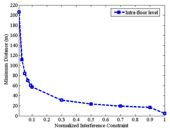
Figure 2.
The optimal minimum distance versus normalized co-channel interference constraint in the intra-floor level.
Assume that , such that by using Equation (2) and Figure 2, the corresponding value of the minimum distance between co-channel interferers in the intra-floor level can be found as , which corresponds to a separation of at least 3 apartments between intra-floor co-channel interferers. Hence, using Equations (6) and (7), = 3, such that . Since the mmWave spectrum can be reused on each floor (i.e., for ), using Equation (8), . Now, using Equation (9), we can find the size of a 3D cluster . Similarly, using Figure 2, the optimal size of a 3D cluster of small cells corresponding to any intra-floor interference value can be estimated. Now, consider that each multistory building consists of 10 floors, each containing 18 apartments, such that the total number of apartments per building is = 180. Now, using Equation (10), the total number times the same mmWave spectrum that can be reused for small cells per building is given by .
4.2. Evaluation Parameters and Assumptions
Default parameters and assumptions used for the system-level evaluation are given in Table 2. To comply with the recommendations of standards bodies [18], omnidirectional path loss models with arbitrary antenna patterns are considered for small cells operating in only mmWave spectra. Further, no small-scale fading is considered at mmWave frequencies due to insignificant small-scale fading variation (e.g., dB) in the mmWave received signals [19]. Furthermore, even though the CIF large-scale model at the 28 GHz band is available for both line-of-sight (LOS and non-line-of-sight (NLOS) signal propagations [18], because there is less multi-path fading at mmWave frequencies in indoor environments, we consider the CIF large-scale LOS model. However, since the path loss exponent in NLOS propagation of mmWave signals increases considerably from that in LOS (e.g., from 2.1 in LOS to 3.4 in NLOS propagation of the 28 GHz signal [18]), the size of an optimal 3D cluster of small cells in a building, in general, would also decrease, particularly at the intra-floor level. Hence, considering NLOS instead of LOS would help improve the overall system-level performance due to reusing the same mmWave spectrum more for NLOS than LOS for each building. In other words, the performance analysis using the LOS 28 GHz mmWave spectrum could be considered as a worst case scenario analysis in this band, which we carry out in this paper. Additionally, since the mmWave path loss indoors is frequency-dependent, which typically increases with an increase in frequency, we consider the lower 28 GHz mmWave path loss model to estimate the optimal 3D cluster size of small cells within a multistory building, which is applicable to both 28 and 60 GHz spectrum bands.
Table 2.
Default parameters and assumptions.
4.3. Performance Analysis
Using the analytical expressions given by Equations (21)–(23) and varying the number of buildings L, as well as the 3D spatial reuse factor given by Equation (10), the impact of applying the proposed technique for 3D spatial reuse of 28 and 26 GHz mmWave spectra to in-building small cells for each building in terms of average SE and average EE is discussed in the following.
4.3.1. Impact of 3D Spatial Reuse of mmWave Spectra
Figure 3 shows SE and EE responses when applying 3D spatial reuse of mmWave spectra to in-building small cells for = 20. It is clear from Figure 3a that with an increase in the number of buildings L, SE increases significantly when employing 3D spatial reuse of spectra to small cells within each building as compared to when no reuse is considered. Employing only horizontal 2D spatial reuse of mmWave spectra, reusing any spectrum just once for each building containing small cells is not sufficient to gain high SE, due to the limitation of the maximum number of multistory buildings that can exist within each macrocell’s coverage. To achieve ultra-high SE (e.g., 10 times the efficiency of 5G networks [1]) for future 6G mobile networks, in addition to the horizontal spatial reuse of spectra by more than one building containing small cells (i.e., L > 1), the vertical (i.e., the £D inter-floor- and intra-floor-level reuse of spectra within a building) spatial reuse of mmWave spectra within each building needs to be exploited.
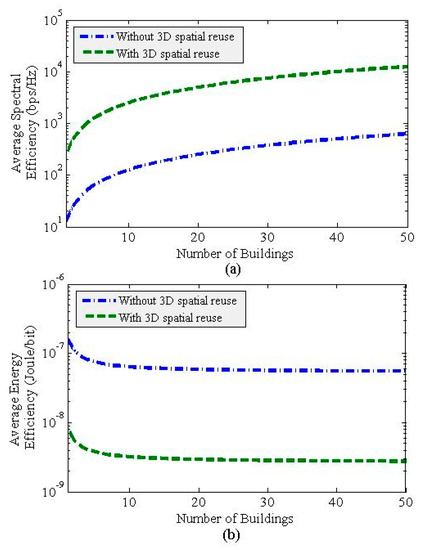
Figure 3.
Impact of applying 3D spatial reuse of mmWave spectra to in-building small cells: (a) system-level average SE; (b) system-level average EE.
By exploiting the vertical spatial reuse of mmWave spectra by small cells within each building, an MNO can address the scarcity of spectrum demands without sharing the spectra of other MNOs or different systems, such as non-terrestrial satellite systems. This can result in saving additional costs and reducing the network complexities associated with sharing spectra with other systems. From Figure 3b, it can be found that EE improves exponentially with an increase in L and becomes almost steady for large values of L. Hence, unlike SE, 3D spatial reuse of spectra within each building of small cells improves EE by a decent margin of about 20 times in the steady-state of the EE response with L as compared to when no 3D spatial reuse of spectra is exploited. In short, exploiting 3D spatial reuse of mmWave spectra within multistory buildings of small cells is a very effective technique to address the expected SE and EE requirements for 6G mobile networks [1,2].
4.3.2. Impact of Variation in 3D Spatial Reuse Factor
Recall that both 28 GHz and 60 GHz mmWave spectra can be reused on each floor. Hence, using Equation (6), the size of a 3D cluster is 1, 4, 9, or 16 for a maximum number of 18 apartments per floor for a 10-story building. However, using Figure 2, it can be found that for a 3D cluster size of 1, needs to be set to 1, which is not feasible, since the maximum value of the normalized desired received signal power of a small-cell UE from its serving small cell is 1. Hence, using Equation (10), a 3D cluster size of 4, 9, or 16 corresponds to value of 35, 20, or 11.25, respectively.
Figure 4 and Figure 5 show SE and EE responses for values of 35, 20, and 11 with the variation in L. From Figure 4a, it can be found that SE improves linearly with an increase in L for any value of . Similarly, SE improves linearly with an increase in for any value of L (Figure 5a). Hence, Figure 4a and Figure 5a imply that SE improves by a factor of (i.e., it is a horizontal and vertical spatial reuse product). However, from Figure 4b and Figure 5b, it can be found that EE improves noticeably with an increase for low values of L (e.g., 1 ≤ L ≤ 5). As L gets larger (e.g., L > 50), no significant improvement in EE is achieved, even though increases from 11 to 35 (Figure 5b). Hence, mainly impacts SE enhancement, irrespective of the values of L, whereas contributes to enhancing EE for low values of L.
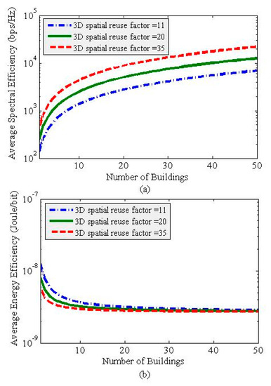
Figure 4.
(a) Average spectral efficiency (SE) and (b) average energy efficiency (EE) responses for numerous 3D spatial reuse factors per building with the variation in the number of buildings of small cells, L.
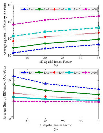
Figure 5.
(a) Average spectral efficiency (SE) and (b) average energy efficiency (EE) responses for different values of L with the variation in 3D spatial reuse factor per building.
4.4. Performance Comparison
According to [25,26], the average SE and average EE requirements for 5G mobile systems are 27–37 bps/Hz and 3 × 10⁻⁶ Joules/bit, respectively. It is expected that the future 6G mobile systems will require 10 times average the SE [1] (i.e., 270–370 bps/Hz) and 10 times the average EE [2] (i.e., 0.3 × 10⁻⁶ Joules/bit) of 5G mobile systems. Here, and denote the average SE and average EE requirements for 6G mobile systems, respectively, such that = 270–370 bps/Hz and = 0.3 × 10⁻⁶ Joules/bit. Now, using Equations (22)–(23), the required values of and L for the system-level average SE and average EE to satisfy the corresponding requirements for 6G mobile systems are given in Table 3. From Table 3, it can be found that both the average SE and average EE requirements for 6G mobile systems can easily be satisfied by all possible 3D spatial reuse factors with cluster sizes of 4, 9, and 16 for multistory buildings, with each building containing 10 floors with 18 apartments per floor, which is achieved by reusing the same 28 and 60 GHz mmWave spectra, with small-cell building L values of just 3, 2, and 1, respectively. It is noted that with no 3D spatial reuse of mmWave spectra (i.e., = 1), a large number of small-cell buildings with L = 30 are needed to satisfy the requirements (particularly, the average SE requirement) for 6G mobile networks.
Table 3.
Required values of 3D spatial reuse factor and the number of small-cell buildings L to satisfy both average SE and average EE requirements for 6G mobile networks.
5. Conclusions
In this paper, unlike previous works (e.g., [9,10,11,12]) that exploited the microwave channel model, by exploiting the 28 GHz mmWave channel model, we have presented a technique for 3D spatial reuse of multi-millimeter-wave (multi-mmWave) spectra in ultra-dense in-building small cells. In doing so, we first present an analytical model for the 28 GHz mmWave spectrum to characterize co-channel interference (CCI) between small cells enabled with dual transceivers operating in 28 and 60 GHz millimeter-wave (mmWave) bands in a multistory building. The 28 GHz mmWave spectrum is considered to model CCI and define a minimum distance between co-channel small cells in both intra- and inter-floor levels, such that finding an optimal size of a 3D cluster of small cells in a building is applicable for both 28 and 60 GHz spectrum bands, due to less indoor propagation loss in the 28 GHz band than in the 60 GHz band. We then define the corresponding 3D spatial reuse factor, such that the entire 28 and 60-GHz spectra can be reused by each 3D cluster in each building. Considering a system architecture where outdoor macrocells and picocells operate in the 2 GHz microwave spectrum, we derive the system-level average capacity, spectral efficiency (SE), and energy efficiency (EE) performance metrics and develop an algorithm for the proposed technique.
Extensive system-level numerical and simulation analysis has been carried out to evaluate the performance of the proposed technique. It has been shown that with an increase in the number of small cell buildings L for a given value of , SE increases significantly when employing 3D spatial reuse of spectra by small cells within each building as compared to when no reuse is considered (i.e., ). This implies that employing horizontal 2D spatial reuse of mmWave spectra only once per small-cell building (i.e., by increasing L) is not sufficient to gain high SE, since L is limited by the macrocell coverage. To achieve ultra-high SE for 6G mobile networks, in addition to the horizontal spatial reuse of spectra, the vertical spatial reuse of mmWave spectra within each building needs to be exploited. In short, the average SE improves by the product of horizontal spatial reuse of mmWave spectrums by varying the number of buildings L and vertical spatial reuse of mmWave spectrums by varying the 3D spatial reuse factor , i.e., .
On the other hand, the average EE improves exponentially with an increase in L and becomes almost steady for large values of L. However, with an increase in , EE improves noticeably for low values of L (e.g., 1 ≤ L ≤ 5). As L gets larger (e.g., L > 50), no significant improvement in EE can be achieved, irrespective of the values of . Hence, mainly impacts SE enhancement, irrespective of the values of L, whereas contributes to enhancing EE only for low values of L. Finally, we have shown that in contrast to considering = 1, which requires L = 30, the expected requirements for 6G mobile networks of 270–370 bps/Hz average SE and 0.3 × 10⁻⁶ Joules/bit average EE can be satisfied with for low values of L (e.g., values of 4, 9, and 16 require L values of just 3, 2, and 1, respectively), with each containing 180 small cells. Hence, 3D spatial reuse of multi-mmWave spectra by small cells deployed within multistory buildings is a promising technique to address the expected average SE and EE requirements for 6G mobile networks.
Funding
This research received no external funding.
Acknowledgments
This paper is partly submitted to the 2020 IEEE 92nd Vehicular Technology Conference (VTC2020-Fall), Victoria, BC, Canada, [27].
Conflicts of Interest
The author declares no conflict of interest.
References
- Zhang, Z.; Xiao, Y.; Ma, Z.; Xiao, M.; Ding, Z.; Lei, X.; Karagiannidis, G.K.; Fan, P. 6G wireless networks: Vision, requirements, architecture, and key technologies. IEEE Veh. Technol. Mag. 2019, 14, 28–41. [Google Scholar] [CrossRef]
- Chen, S.; Liang, Y.; Sun, S.; Kang, S.; Cheng, W.; Peng, M. Vision, requirements, and technology trend of 6G: How to tackle the challenges of system coverage, capacity, user data-rate and movement speed. IEEE Wirel. Commun. 2020, 1–11. [Google Scholar] [CrossRef]
- Yang, P.; Xiao, Y.; Xiao, M.; Li, S. 6G wireless communications: Vision and potential techniques. IEEE Netw. 2019, 33, 70–75. [Google Scholar] [CrossRef]
- Saad, W.; Bennis, M.; Chen, M. A vision of 6G wireless systems: Applications, trends, technologies, and open research problems. IEEE Netw. 2019, 1–9. [Google Scholar] [CrossRef]
- Zhao, J.; Ni, S.; Yang, L.; Zhang, Z.; Gong, Y.; You, X. Multiband cooperation for 5G hetnets: A promising network paradigm. IEEE Veh. Technol. Mag. 2019, 14, 85–93. [Google Scholar] [CrossRef]
- Song, H.; Fang, X.; Yan, L.; Fang, Y. Control/user plane decoupled architecture utilizing unlicensed bands in LTE systems. IEEE Wireless Commun. 2017, 24, 132–142. [Google Scholar] [CrossRef]
- Mohamed, A.; Onireti, O.; Imran, M.A.; Imran, A.; Tafazolli, R. Control data separation architecture for cellular radio access networks: A survey and outlook. IEEE Commun. Surveys Tuts. 2016, 18, 446–465. [Google Scholar] [CrossRef]
- Mohamed, A.; Onireti, O.; Imran, M.A.; Imran, A.; Tafazolli, R. Predictive and core-network efficient RRC signalling for active state handover in RANs with control/data separation. IEEE Trans. Wireless Commun. 2017, 16, 1423–1436. [Google Scholar] [CrossRef]
- Saha, R.K.; Aswakul, C. A tractable analytical model for interference characterization and minimum distance enforcement to reuse resources in three dimensional in building dense small cell networks. Int. J. Commun. Syst. 2017, 30, e3240. [Google Scholar] [CrossRef]
- Saha, R.K. Realization of licensed/unlicensed spectrum sharing using eicic in indoor small cells for high spectral and energy efficiencies of 5g networks. Energies 2019, 12, 2828. [Google Scholar] [CrossRef]
- Saha, R.K. Multi-band spectrum sharing with indoor small cells in hybrid satellite-mobile systems. In Proceedings of the 2019 IEEE 90th Vehicular Technology Conference (VTC2019-Fall), Honolulu, HI, USA, 22–25 September 2019; pp. 1–7. [Google Scholar]
- Saha, R.K. A technique for massive spectrum sharing with ultra-dense in-building small cells in 5g era. In Proceedings of the 2019 IEEE 90th Vehicular Technology Conference (VTC2019-Fall), Honolulu, HI, USA, 22–25 September 2019; pp. 1–7. [Google Scholar]
- Allan, R. Application of FSS Structures to Selectively Control the Propagation of Signals into and out of Buildings—Executive Summary; ERA Technology Ltd.: Leatherhead, UK, 2004; Available online: https://www.ofcom.org.uk/__data/assets/pdf_file/0020/36155/exec_summary.pdf (accessed on 25 February 2020).
- Propagation Data and Prediction Methods for the Planning of Indoor Radiocommunication Systems and Radio Local Area Networks in the Frequency Range 300 MHz to 450 GHz. Recommendation ITU-R P.1238-10, 08/2019. Available online: https://www.itu.int/rec/R-REC-P.1238 (accessed on 25 February 2020).
- Lu, D.; Rutledge, D. Investigation of indoor radio channels from 2.4 GHz to 24 GHz. In Proceedings of the IEEE Antennas and Propagation Society International Symposium. Digest. Held in Conjunction with: USNC/CNC/URSI North American Radio Sci. Meeting (Cat. No.03CH37450), Columbus, OH, USA, 22–27 June 2003; Volume 2, pp. 134–137. [Google Scholar]
- Zhao, H.; Mayzus, R.; Sun, S.; Samimi, M.; Schulz, J.K.; Azar, Y.; Azar, Y.; Wang, K.; Wong, G.N.; Gutierrez, F.; et al. 28 GHz millimeter wave cellular communication measurements for reflection and penetration loss in and around buildings in New York city. In Proceedings of the 2013 IEEE International Conference on Communications (ICC), Budapest, Hungary, 9–13 June 2013; pp. 5163–5167. [Google Scholar]
- Ellenbeck, J.; Schmidt, J.; Korger, U.; Hartmann, C. A concept for efficient system-level simulations of OFDMA systems with proportional fair fast scheduling. In Proceedings of the 2009 IEEE Globecom Workshops, Honolulu, HI, USA, 30 November–4 December 2009; pp. 1–6. [Google Scholar]
- Maccartney, G.R.; Rappaport, T.S.; Sun, S.; Deng, S. Indoor office wideband millimeter-wave propagation measurements and channel models at 28 and 73 ghz for ultra-dense 5G wireless networks. IEEE Access 2015, 3, 2388–2424. [Google Scholar] [CrossRef]
- Rappaport, T.S. Millimeter wave mobile communications for 5G cellular: It will work! IEEE Access 2013, 1, 335–349. [Google Scholar] [CrossRef]
- Evolved Universal Terrestrial Radio Access (E-UTRA); Radio Frequency (RF) System Scenarios. Document 3GPP TR 36.942, V.1.2.0, 3rd Generation Partnership Project. July 2007. Available online: https://portal.3gpp.org/desktopmodules/Specifications/SpecificationDetails.aspx?specificationId=2592 (accessed on 15 February 2020).
- Simulation Assumptions and Parameters for FDD HeNB RF Requirements. Document TSG RAN WG4 (Radio) Meeting #51, R4-092042, 3GPP. May 2009. Available online: https://www.3gpp.org/ftp/tsg_ran/WG4_Radio/TSGR4_51/Documents/ (accessed on 13 February 2020).
- Geng, S.; Kivinen, J.; Zhao, X.; Vainikainen, P. Millimeter-wave propagation channel characterization for short-range wireless communications. IEEE Trans. Veh. Technol. 2009, 58, 3–13. [Google Scholar] [CrossRef]
- Saha, R.K.; Saengudomlert, P.; Aswakul, C. Evolution toward 5G mobile networks-A survey on enabling technologies. Eng. J. 2016, 20, 87–119. [Google Scholar] [CrossRef]
- Guidelines for Evaluation of Radio Interface Technologies for IMT-2020. Report ITU-R M.2412-0 (10/2017), Geneva. 2017. Available online: https://www.itu.int/dms_pub/itu-r/opb/rep/R-REP-M.2412-2017-PDF-E.pdf (accessed on 13 February 2020).
- Wang, C.-X.; Haider, F.; Gao, X.; You, X.-H.; Yang, Y.; Yuan, D.; Aggoune, H.; Haas, H.; Fletcher, S.; Hepsaydir, E. Cellular architecture and key technologies for 5G wireless communication networks. IEEE Commun. Mag. 2014, 52, 122–130. [Google Scholar] [CrossRef]
- Auer, G.; Giannini, V.; Desset, C.; Godor, I.; Skillermark, P.; Olsson, M.; Imran, M.; Sabella, D.; Gonzalez, M.; Blume, O.; et al. How much energy is needed to run a wireless network? IEEE Wirel. Commun. 2011, 18, 40–49. [Google Scholar] [CrossRef]
- Saha, R.K. Modeling interference to reuse millimeter-wave spectrum to in-building small cells toward 6G. In Proceedings of the 2020 IEEE 92nd Vehicular Technology Conference (VTC2020-Fall), Victoria, BC, Canada, 4–7 October 2020. [Google Scholar]


© 2020 by the author. Licensee MDPI, Basel, Switzerland. This article is an open access article distributed under the terms and conditions of the Creative Commons Attribution (CC BY) license (http://creativecommons.org/licenses/by/4.0/).