Experimental and Numerical Study on Flow Resistance and Bubble Transport in a Helical Static Mixer

Abstract

Flow resistance and bubble transport in a helical static mixer were studied experimentally and numerically. The inline mixer increases the volume fraction of gas in liquids by breaking bubbles into smaller sizes with a micrometer size in the flow experiments. The gas–liquid flow was simulated by a combination of computational fluid dynamics and Taylor expansion methods of moments. The friction factor of the helical static mixer is much smaller than that of the Kenics static mixers. The pressure drop increases with the Reynolds number, and the increment is larger when the Reynolds number is higher. The equidistant pressure drop increases with the argument of Reynolds number, and increases when the pitch decreases from upstream to downstream. The energy expenditure increases significantly when the variable-pitch coefficient is too small. The bubble geometric mean diameter decreases and the geometric standard deviation increases when the gas–liquid fluid flows through the mixer. The variable pitch structure enhances the bubble breakup effectively. The change of the bubble size decreases with the argument of the Reynolds number. The effect of the mixer has a limitation on breaking the bubbles.

1. Introduction

Mixing is one of the core unit operations performed to enhance heat and mass transfer or chemical reactions for multiphase or multicomponent dispersions in modern industrial processes. In recent decades, developments have been made on the design principles and methods of different kinds of mixing equipment for various process objectives, such as fine chemicals, agrochemicals, pharmaceuticals, cosmetics, food, drinking water and wastewater treatment [1]. A wide range of mixing equipment is now available including static mixers, mechanically stirred vessels/tanks, rotor-stator devices, etc. Micromixers were designed recently which can be used under small Reynolds number as a lab-on-a-chip technology [2]. Static mixers refer to mixing devices that are motionless, and the fluid inside moves in pipelines. Traditional static mixers are made up of a series of metal baffles such as twists of metal, corrugated sheets, parallel bars, small-diameter passages, etc. Multiphase mixing is achieved by redirecting the flow patterns in pipelines [3]. It is a passive mixing method without an external energy source and moving parts, which makes the device easy to manufacture and operate. The static mixer with a helical structure or corrugated sheets is suggested as the best design choice for gas–liquid dispersion applications [1,4].

Static mixers can be divided into three categories based on different mechanisms, which are split-and-recombine [5], chaotic fluid motion by surface patterning [6] and secondary flow in curved channels [7]. Ghanem et al. [8] summarized recent developments on different kinds of industrial static mixers and pointed out that computational fluid dynamics (CFD) facilitated the conceptual designs and the refinement of the static mixers. Energy expenditure, as well as fouling resistance, corrosion, maintenance, and cleaning operations are currently problems in traditional mixing devices. Kenics static mixers (KSM), first manufactured by Chemineer, Inc., consists of a number of elements of alternating 180° helices [9], as shown in Figure 1a. The inserted twisted tapes elongate the inline flow path and reduce the hydraulic diameter, which can enhance the heat and mass transfer. Nevertheless, the flow resistance increases as well [4]. Therefore, many researchers investigated and optimized the hydrodynamic and mixing performance of static mixers with helical flow channels in recent years [10]. Lei et al. [11] numerically studied the fluid flow and heat transfer of pipe flow in a modified helical static mixer with perforated holes on the staggered twisted tapes (Figure 1b). The results showed that the friction factors of flow decreased by 8% to 15.1%, while the heat transfer was enhanced by 34.1% to 46.8%. Meng et al. [3] found that an increase of perforated spacing did not affect the Nusselt number and the friction factor of fluid flow. Rahimi et al. [12] compared different static mixers with four different twisted tapes. They concluded that the jagged twisted tape showed better thermal-hydraulic performance than the typical twisted tape (TTT) (Figure 1c), the perforated twisted tape (PTT) and the notched twisted tape (NTT). Edgefold-twisted tape (ETT) was inserted in the tube and tested by Cui and Tian [13], the results showed that both of the Nusselt number and the friction factor are larger than those of the TTT [14]. Thianpong et al. [15] experimentally studied the heat transfer and friction factor of flow in a tube equipped with the PPT. Compared to the TTT, the mixer with s/W = 0.4, d/W = 0.17, and y/W = 3 achieved heat transfer enhancement up to 27.4%. Eiamsa-ard et al. [16] set twin delta-wings at the twisted tape and tested the friction factor of the inside fluid flow. All of the three different arrangements of twin-wings provided superior thermal performance than the TTT. The friction factor of the TTW-up with wing-tip angle of 20 ° is 8.55 times those of the plain tube.

The kinds of literature reviewed above discussed the overall hydrodynamic and heat transfer assessment of the mixer’s performance. Few studies reported on the gas–liquid dispersion inside the static mixers. Enhanced gas–liquid dispersion can increase the rate of interphase mass transfer and chemical reaction in modern industrial applications [4,17]. Over the last decades, developments have been made on design principles and methods of different kinds of equipment for various applications, such as food, sparkling water, wastewater treatment, fine chemicals, agrochemicals, pharmaceuticals and cosmetics, etc. Furthermore, a static mixer can be used as a microbubble generator utilizing the hydrodynamic shear when gas–liquid fluid flowing through. The hydrodynamic air dispersing method refers to breaking up bubbles using a high-speed shear into microbubbles (d < 50 μm), which can be dispersed into liquid phase stably [18]. This method has the advantage of low energy-consumption, high efficiency for mixing and mass transfer, and is environmentally friendly compared to other methods such as ultrasonic cavitation [19], chemical reaction or electrolysis [20,21]. As early as 1961, Turner et al. [19] first discovered that ultrasonic cavitation can generate microbubbles with 30 μm in water and can be stored for more than 100 h. However, this method is unable to work continuously, and the power consumption is relatively large with low efficiency. Other methods with high cost are generating microbubbles by chemical reaction or electrolysis. Lawrie et al. [20] obtained a large number of oxygen microbubbles with an average diameter of 3 μm by segmenting hydrogen peroxide. However, the use of chemical reagents can easily cause pollution. Osamu et al. [21] electrolyzed a large number of microbubbles with an average diameter of 777 nm in water by a mesh electrode made by metal microfibers with diameter of 200 μm. However, the production of microbubbles by such a kind of method is low. Releasing dissolved gas in liquid is a popular way to generate abundant micro-nano bubbles in recent years. The key to the system is the design of a flow channel and releaser. For example, the SMX-155 bubble generator (Riverforest Inc., California, USA) can produce microbubbles with a diameter within 5 to 30 μm. The dissolved gas releasing method is economical and productive. However, the preparation of dissolved gas in liquid relies on high pressure. The BUSP series products (Honda Pumps Inc., Fukuoka, JAPAN) disperses air into bubbles with a diameter range from 1 to 50 μm by a high-speed stirring of an impeller in water. The maximum gas volume fraction can up to 7% and the flow rate up to 360 m³/h [22]. Different arrangements of static mixer elements were tested in a horizontal pipe by Heyouni et al. [23]. They found the change of bubbles diameters depend on liquid velocity, gas velocity and also on the structure of the static mixer. Nevertheless, correlations were given for the prediction of the bubble diameters without considering the effect of element numbers. The gas–liquid flow in a vertical pipe packed with a helical static mixer was characterized by Rabha et al. [4]. The ultrafast electron beam X-ray tomography is used to determine the gas–liquid flow structure. They found that the bubble diameter correlations for KSM are not suited for adequate predictions in the gas–liquid vertical up-flow. The number of mixer elements and the mixer geometric characteristics significantly affect the bubble breakup. Euler–Euler simulations were done by Zidouni et al. [17] to investigate the gas–liquid two-phase flow. Bubble distribution in gas–liquid flows can be predicted by some existing models, but the research simplified the bubble size distribution as a mono-disperse. The swirling flow induced by the helical mixer elements can cause phase separation and the gas can concentrate in the center of the tube. This effect is unbeneficial to the gas–liquid contacting and mixing. Putra et al. [24] measured the gas volume fractions at several planes within the swirl element using high-resolution gamma-ray computed tomography (HireCT). Three flow regions namely the bubbly flow region, transition region, and gas core region can be found in the flow domain. The bubble size influenced the peak location of gas radial fraction differently in these regions.

Most of the experimental works on static mixers have concentrated on establishing design guidelines and pressure drop correlations. The number of investigations into the flow and mixing mechanisms is limited, probably due to difficulties encountered in obtaining meaningful experimental measurements. Bubble coalescence and breakup are the main phenomena for gas–liquid fluid flow inside the devices [25]. Recently, Falzone et al. [26] concluded four main mechanisms leading to bubble breakup, which were turbulent fluctuation, macroscopic shear stress, turbulent shear stress and interfacial slip. A computational fluid dynamics-population balance model (CFD-PBM) framework has been proven effective to predict the local bubble size distribution (BSD) in fluid flow. Martinez et al. [27] indicated that the existing models for bubble breakup were nearly identical and size of bubbles decreases as a properly defined Weber number. Their simulations showed that binary models with ∩—shapes predicted the daughter size PDF well according to the experimental data. Tran-Cong et al. [28] observed the transverse ‘migration’ of mono-disperse bubbles by flow visualization, they found that the migration only takes place for small bubbles (d < 3.5 mm) and is shown to be non-systematic. Azizi and Al Taweel [29] simulated gas–liquid contacting based on the classical phenomenological model developed by Coulaloglou and Tavlarides [30], the giving Sauter-mean-diameter showed good agreement with experimental results. Bubble dispersion in a twin-screw continuous mixer was studied experimentally and numerically by Vyakaranam and Kokini [31], FEM simulation results indicated that the maximum stable bubble diameter in the mixer agrees with half of the experimental data. Nguyen et al. [32] proposed a new model for bubble coalescence and break-up considering turbulent suppression, and the model showed improvements and can apply to high liquid velocity condition of turbulent bubbly two-phase flow. Chouippe et al. [33] observed bubble accumulation through a numerical study on bubble dispersion in turbulent Taylor–Couette flow. Bubbles rise through the vortices along helix lines of the inner cylinder when vortex trapping was dominated by buoyancy. Diffusion Inertia Model and δ—function approximation are used by Mukin [34] to consider interphase momentum transfer between bubble and liquid, the proposed model is validated by flow loop experiments. Liao et al. [35] developed a baseline closure model for adiabatic poly-disperse bubbly flow, data revealed that the model describes BSD well without any adjustment. Hereafter, they proposed an alternative discrete formulation of the PBE for the binary breakup, which is better than previous models made by Kumar and Ramkrishna [36]. A large-eddy simulation of microbubble transport in a turbulent horizontal channel flow was performed by Asiagbe et al. [37], and the results showed that low-density microbubbles migrated towards the upper channel wall under the driven of buoyancy.

In this study, a new type of static mixer without baffles was studied. Experiments were performed for measuring the pressure drop and bubble transport in the helical static mixer. A numerical model was built for the gas–liquid two-phase flow based on the PBM-CFD method. Simulations of a 3D model were performed to analyze the flow characteristics and BSD and find out the effects of Reynolds number and variable-pitch coefficient.

2. Experimental Setup

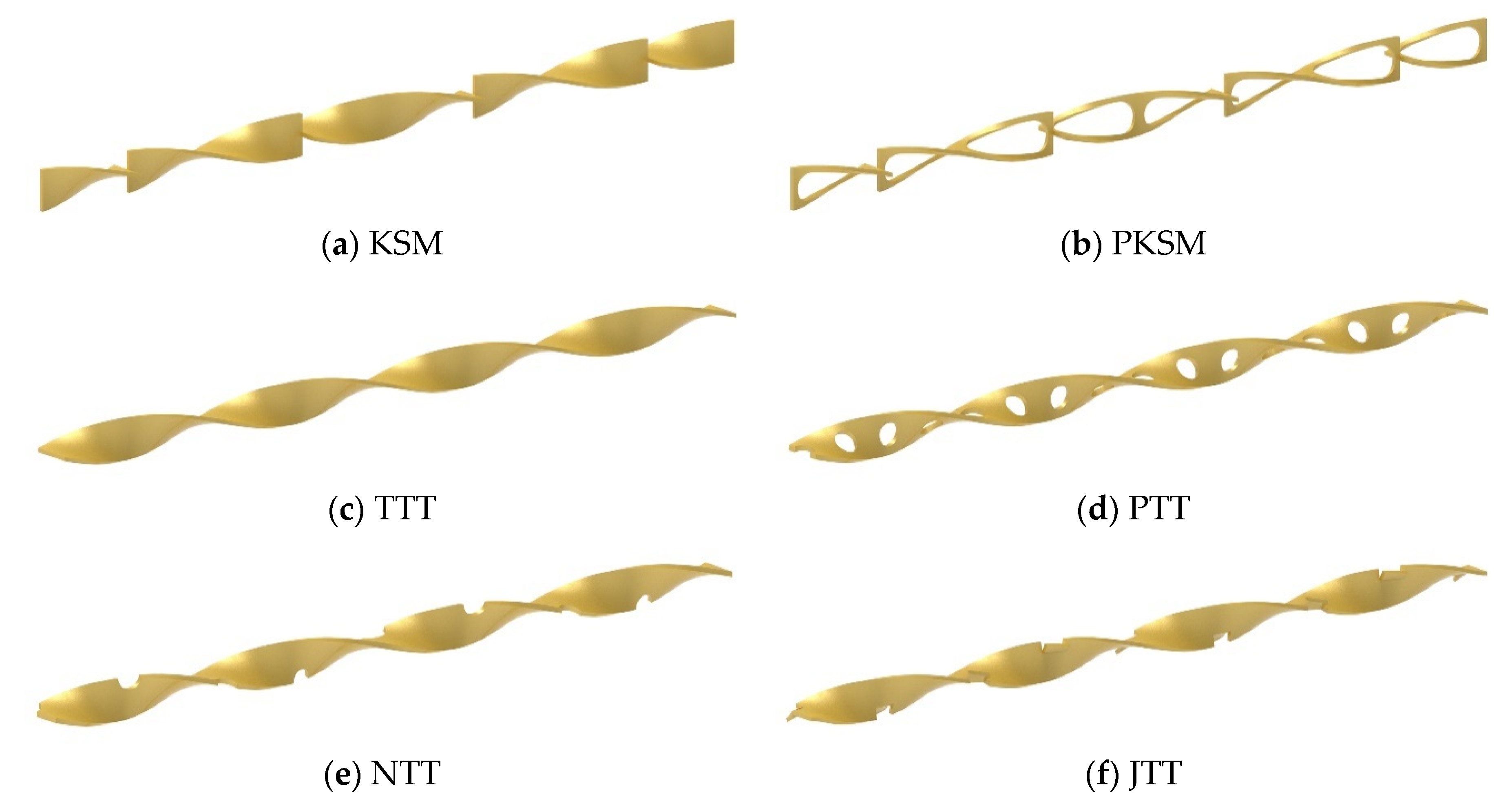
2.1. Structure of the Helical Static Mixer

Figure 2 shows the main structure of the newly developed helical static mixer. The helical cavity core is assembled by stacking over 4000 thin steel sheets with a thickness of 0.08 mm (Figure A1 in Appendix A) along with a specific helix equation:

$$\{\begin{array}{l}x=R\cos \theta \\ y=R\sin \theta \\ z=l{\left(\theta /2\pi \right)}^m\end{array}$$

(1)

where R is the radius of thin sheets, θ is the torsion angle range from 0 to 2π. l is the length of the helical cavity core (280 mm in this study). The inner and outer diameters of the HSM are 12 mm and 25 mm, respectively. The width of the cross steel sheets is 6 mm. Hence, the porosity is about 68.5% according to the dimension of cross section in Figure A1 Appendix A. The characteristics of the typical static mixers are listed in

Table 1. Characteristics of the typical static mixers.

Static Mixer Design	Diameter (mm)	Mixing Length (mm)	Number of Elements	Global Porosity (%)
KSM (Chemineer Inc., Ohio, USA) [38]	19.1	687.6	24	78
PKMS [3]	40	960	12	90.8–93.3
SMV (Sulzer Inc. Winterthur, Switzerland) [39]	10	50	5	83
SMX+ (Sulzer Inc.) [40]	5	50	10	75
TTT [16]	19	1000	1	94.6
Current HSM	25	280	1	68.5

. Several common types of static mixers are presented as a comparison. The helical static mixer (HSM) has the advantages of the TTT and the SMV, which is the design with an integrated helical structure and a series of ridges. The porosity of the device is smaller than the other commercial mixers because the HSM is under test and the structure has not been optimized yet. The HSM is designed as a variable-pitch with a constant coefficient m, which is the most obvious difference between the other mixers. The mixer is an inline device that can be mounted statically in the pipeline by flanges on the casing (Figure A2 in Appendix A). The inside fluid flows through the mixer from the inlet with a large pitch to the outlet with a small pitch. The unique structure of the device divides four separated helical flow channels with cross-sections in sector shape. The inside and outside arc surfaces are smooth, but two side surfaces along the channels consist of a pair of continuous steps with varying step heights. Baffles in traditional mixing devices are replaced by thousands of frontward-facing and backward-facing micro-sized steps to generate hydrodynamic turbulence, so as to enhance gas–liquid contact and dispersion. The variable-pitch coefficient can be adjusted flexibly when manufacturing. Flow experiments and numerical studies are performed hereinafter to evaluate the performance of the newly developed static mixer.

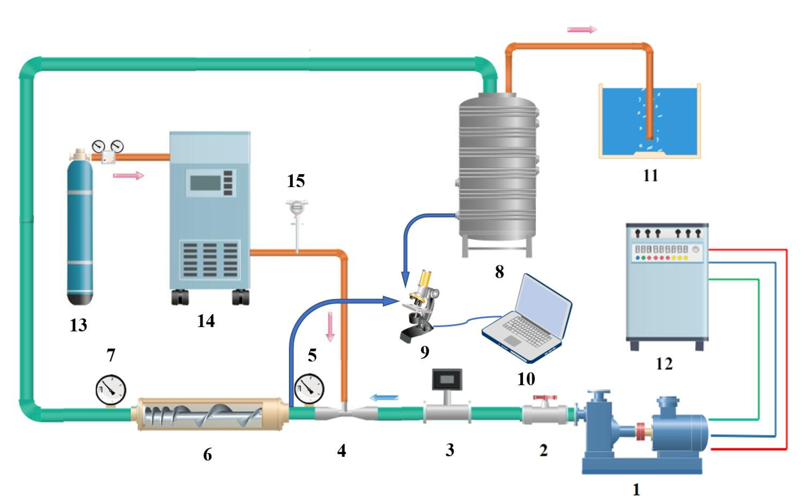
2.2. Experimental Setup

The schematic of the experimental setup is shown in Figure 3. A centrifugal pump provides output power controlled by the control box to drive the fluid flow. The valve controls the flow rate. Venturi nozzle disperses the gas from the cylinder into millimeter-sized bubbles before entering the helical static mixer. Then, the bubbles are broken up inside the mixer and the obtained suspensions are stored in the tank.

A microscope made by Keyence VHX-5000 is used for observing bubbles dispersed in the water. The highest resolution of the microscope is up to 0.5 μm. Figure 4b gives the picture taken by a microscope in which the bubble size is at the micrometer level. It is approximately three orders of magnitude less than the initial bubble size that is at the millimeter level. Microbubbles dispersed in liquid possess large surface areas—far greater than visible large bubbles. Furthermore, smaller bubbles are easier to suspend in liquid with longer residence time [18]. The size distributions of bubbles in suspensions before and after the mixing process were determined using the Image Particle Size analyzer (Model BT-1600) from Bettersize Inc., China, which employs a software particle image processing technology that provides intuitive and accurate analyses. The measured data are compared to the numerical results.

3. Numerical Model

3.1. Fluid Flow

A one-way coupling model for gas–liquid two-phase flow is built considering the light-loading of the bubbles. The variation of bubble volume is neglected due to little change of hydrodynamic pressure along the flow direction. The governing continuity and Reynolds-averaged Navier–Stokes (RANS) equations for incompressible fluid flow are:

$$\frac{\partial {\overline{u}}_i}{\partial x_i}=0$$

(2)

$$\frac{\partial {\overline{u}}_i}{\partial t}+\frac{\partial \overline{u_i{u}_j}}{\partial x_j}=-\frac{1}{\rho }\frac{\partial \overline{p}}{\partial x_i}+\upsilon \frac{{\partial }^2{\overline{u}}_i}{\partial x_j\partial x_j}$$

(3)

in which u_i, p, and ρ are the velocity, pressure, and density of fluid flow, respectively. $\overline{u_i{u}_j}$ is the Reynolds stress and can be solved by turbulence models. Subscripts i and j represent coordinate components. The overbar on the variables represents time-averaged components. SST k-ω model is used in this study because the model predicts the flow separation well in the presence of the adverse pressure gradient [41].

3.2. Bubble Transport

The transport of bubbles dispersed in the fluid is governed by the bubble population balance equation including the coalescence and breakup behaviors of bubbles [26,42]:

$$\begin{array}{ll}\frac{\partial n(v,t)}{\partial t}+\frac{\partial }{\partial x_i}\left(n(v,t){\overline{u}}_i\right)=& -\frac{\partial }{\partial v}(\frac{\partial v}{\partial t}n(v,t))\\ & +\frac{1}{2}{\displaystyle \underset{0}{\overset{v}{\int }}\beta (v_1,v)n(v_1,t)n(v,t)d{v}_1}-n(v,t){\displaystyle \underset{v}{\overset{\infty }{\int }}\beta (v_1,v)}n(v_1,t)d{v}_1\\ & +{\displaystyle \underset{v}{\overset{\infty }{\int }}a(v_1)b(v|v_1)}n(v_1,t)d{v}_1-a(v)n(v,t)\end{array}$$

(4)

where n(v,t) is the bubble number density function, v and v₁ are bubble volumes, β(v,v₁) is the coalescence kernel which describes the collision frequency of bubbles with volume v and v₁. α(v) is the breakup kernel that gives the frequency of breakup of bubbles of volume v, and b(v|v₁) is the breakup distribution function. The first term on the right-hand side (RHS) of Equation (4) represents the dissolution effect which is ignored here because the process is very short and the solubility is low [27]. The second and third terms on the RHS of Equation (4) describes the birth and death of bubbles because of coalescence, and the fourth and fifth terms give the birth and death of bubbles because of breakup, respectively. Due to the large Reynolds number, the coalescence of bubbles is dominated by turbulence, and the turbulent coalescence kernel is [43]:

$${\beta }_t\left(v,v_1\right)={\left(9/10\pi \right)}^{1/2}G{\left(v^{1/3}+v_1^{1/3}\right)}^3$$

(5)

where G is the local shear rate and equals to (ε/υ)^1/2, and υ is the kinematic viscosity and ε is the turbulent dissipation rate. Thousands of steps cause flow separation near the wall and induce adequate shear stress in the flow field, which leads to bubble breakup into smaller sizes [42,44]. In this study, the shear-induced breakup kernel proposed by Barthelmes et al. [45] is used for describing bubble breakup, because the model considers the bubble size, shape and volume fraction:

$$a(v)=\varsigma v^{1/3}$$

(6)

where the coefficient $\zeta =k{(\frac{{\eta }_{tot}G}{{\tau }^{\ast }})}^q{(\frac{d_c(v)}{d})}^{3/D_f}$, in which k is 1 m⁻³s⁻¹ to match the dimensions of the model, η_tot is the effective viscosity of suspension and d_c is the characteristic diameter of the bubble. D_f is the fractional dimension of bubbles. τ* is the characteristic shear stress which equals 0.00051. q is a constant equal to 1.6. Breakup distribution function b(v|v₁) employs the binary breakup daughter bubble distribution function:

$$b(v|v_1)=\{\begin{array}{cc}2& if v_1=2v\\ 0& others\end{array}$$

(7)

Substituting Equations (5)–(7) into Equation (4), then multiplying the equation by v^k and integrating over the entire size distribution, the bubble population balance equation is transformed to moment equation based on the particle volume:

$$\begin{array}{c}\frac{\partial m_k}{\partial t}+\mathbf{u}\cdot \nabla m_k=\frac{1}{2}{\displaystyle \underset{0}{\overset{\infty }{\int }}{\displaystyle \underset{0}{\overset{\infty }{\int }}[{(v_1+v_2)}^k-v_1^k-v_2{}^k]\beta (v_1,v_2)n(v_1,t)n(v_2,t)d{v}_{1}d{v}_2}}\\ +{\displaystyle \underset{0}{\overset{\infty }{\int }}{\overline{b_i}}^k}a(v_1)n(v_1,t)d{v}_1-{\displaystyle \underset{0}{\overset{\infty }{\int }}{v}^{k}a(v)n(v,t)}dv\end{array}$$

(8)

where $\overline{b_i^k}={\int }_0^{\infty }{v}^{k}b\left({v|v}_1\right)dv=2^{1-k}{v}_i^k$, and the kth order of moment is defined as:

$$m_k={\displaystyle \underset{0}{\overset{\infty }{\int }}{v}^{k}n(v)dv}$$

(9)

The first term on the RHS of Equation (8) is nonlinear and can be solved by the Taylor expansion method of moments (TEMOM) proposed by Yu et al. [46]. This method has no prior requirement for bubble size distribution and was proved able to obtain the evolution of bubble size distribution efficiently [47]. Simplifying Equation (8) by TEMOM and a group of ordinary differential equations with three equations and three unknown moments is obtained:

$$\begin{array}{l}\frac{\partial m_0}{\partial t}+\mathit{u}\cdot \nabla m_0=-\frac{A}{27}\left(\frac{-20m_2{m}_1^2{m}_0^2+127m_1^4{m}_0+m_2^2{m}_0^3}{m_1^3}\right)-\frac{\varsigma }{9}\left(\frac{m_0^{5/3}{m}_2-10m_0^{2/3}{m}_1^2}{m_1^{5/3}}\right)\\ \frac{\partial m_1}{\partial t}+\mathit{u}\cdot \nabla m_1=0\\ \frac{\partial m_2}{\partial t}+\mathit{u}\cdot \nabla m_2=\frac{4A}{27}\left(\frac{35m_2{m}_1^2{m}_0+14m_1^4+5m_2^2{m}_0^2}{m_1{m}_0}\right)-\frac{\varsigma }{18}\left(\frac{14m_0{m}_1^{1/3}{m}_2-5m_1^{7/3}}{m_0^{4/3}}\right)\end{array}$$

(10)

in which the coefficient A = (9/10π)^1/2G.

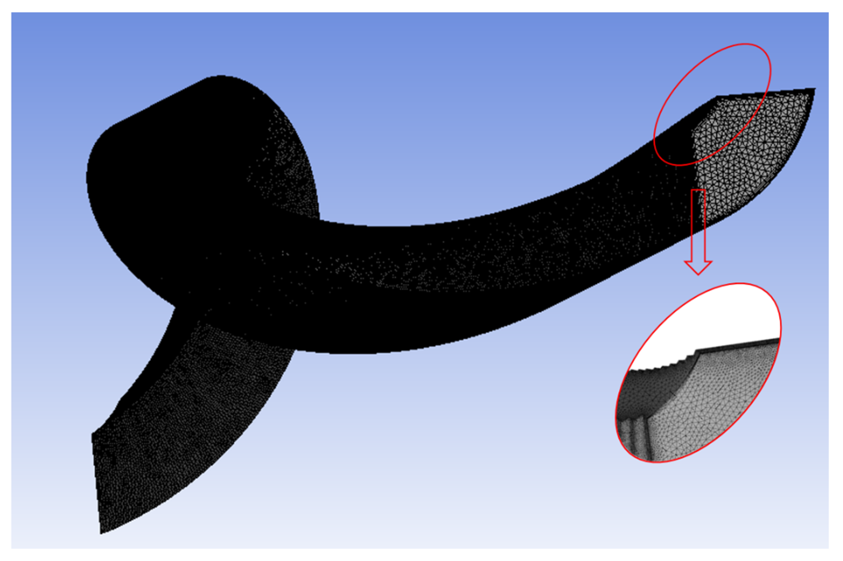
3.3. Computational Domain and Mesh Generation

Four separate flow channels in the helical static mixer are rotationally symmetric, so a single flow channel is picked up to perform the simulation. In Figure 5, a three-dimensional computational domain with numerical mesh edges is shown for numerical study. The step heights are determined by specific helix line equations according to Equation (1). The unstructured tetrahedral mesh system with 1e+7 nodes (Grid 2) is selected for numerical calculations after a grid independency test (Re = 22,392) shown in

Table 2. Grid independency test.

Grid Name	Number of Elements (104)	Pressure Drop (Pa)	Relative Error of Pressure Drop (%)
Grid 1	1845	3352.4	-
Grid 2	1074	3318.8	1.0
Grid 3	552	3228.4	3.7
Grid 4	385	3007.1	10.3

. The grids near the steps are set dense according to the estimated wall spacing based on y+.

3.4. Flow Parameters and Boundary Conditions

The continuous phase for fluid flow is water, with density ρ_l = 998.2 kg·m⁻³, μ = 1.003·10⁻³ Pa·s. The oxygen is chosen as the gas phase with density ρ_g = 1.4 kg·m⁻³ as it is hardly soluble in water. It was found that bubble dispersion is influenced by inlet flux of gas and water, and the inlet pressure of gas and water. Yu et al. [48] found that the volume fraction of gas dispersed in water increased up to 47.12 mg/L when the water and gas flow rates are Q_l = 10 L/min and Q_g = 0.9 L/min, respectively. The results showed that the gas holdup is 26.5% more than the data before experiments and beyond the solubility in water. The slip ratio of inlet velocity (velocity of bubbles to water) is set as 80%. The initial values of moments are determined by the fitted bubble size distribution at the inlet: $m_{k0}=m_{00}{v}_{g0}^{k}exp\left(9k^{2}l{n}^2{\sigma }_{g0}/2\right)(k = 0,1,2)$, where v_g0 and σ_g0 are the initial average volume and geometric standard deviation (GSD) of the bubbles. These moment variables are dimensionless during the calculation to avoid divergence because the orders of magnitudes are too large or too small. The outlet of the domain is set as a pressure-outlet to ensure the stability of the calculation. Both of the frontward-facing and backward-facing steps fit for wall boundary conditions with no-slip for velocity and zero flux for moments. The simulations are performed in parallel computing using the commercial CFD software ANSYS Fluent 19.0. The second-order algorithm and schemes are used and the no-slip condition is set for wall boundary condition.

4. Results and Discussion

4.1. Verification

To validate the model and experimental setup, friction factors of single-phase turbulent flows in an open pipe are compared with the theoretical curve. The Reynolds number is defined as Re = ρ_wV₀D/μ_w, and the friction factor is defined as f = ΔP/(2ρ_wV₀²L/D), where ΔP is the pressure drop between the pipe inlet and the outlet. Figure 6 shows the comparison of the friction factors varying with the Reynolds number. The curve is the Blasius equation which is f = 0.3164Re^−0.25 for turbulent flows. The numerical results are consistent with the Blasius solution. The experimental data are slightly larger than the theoretical solution and numerical results with a maximum difference of about 5%, which may be induced by the entrance region effect [49]. The measurement system and numerical model are verified useful to predict the internal pipe flow.

4.2. Flow Resistance

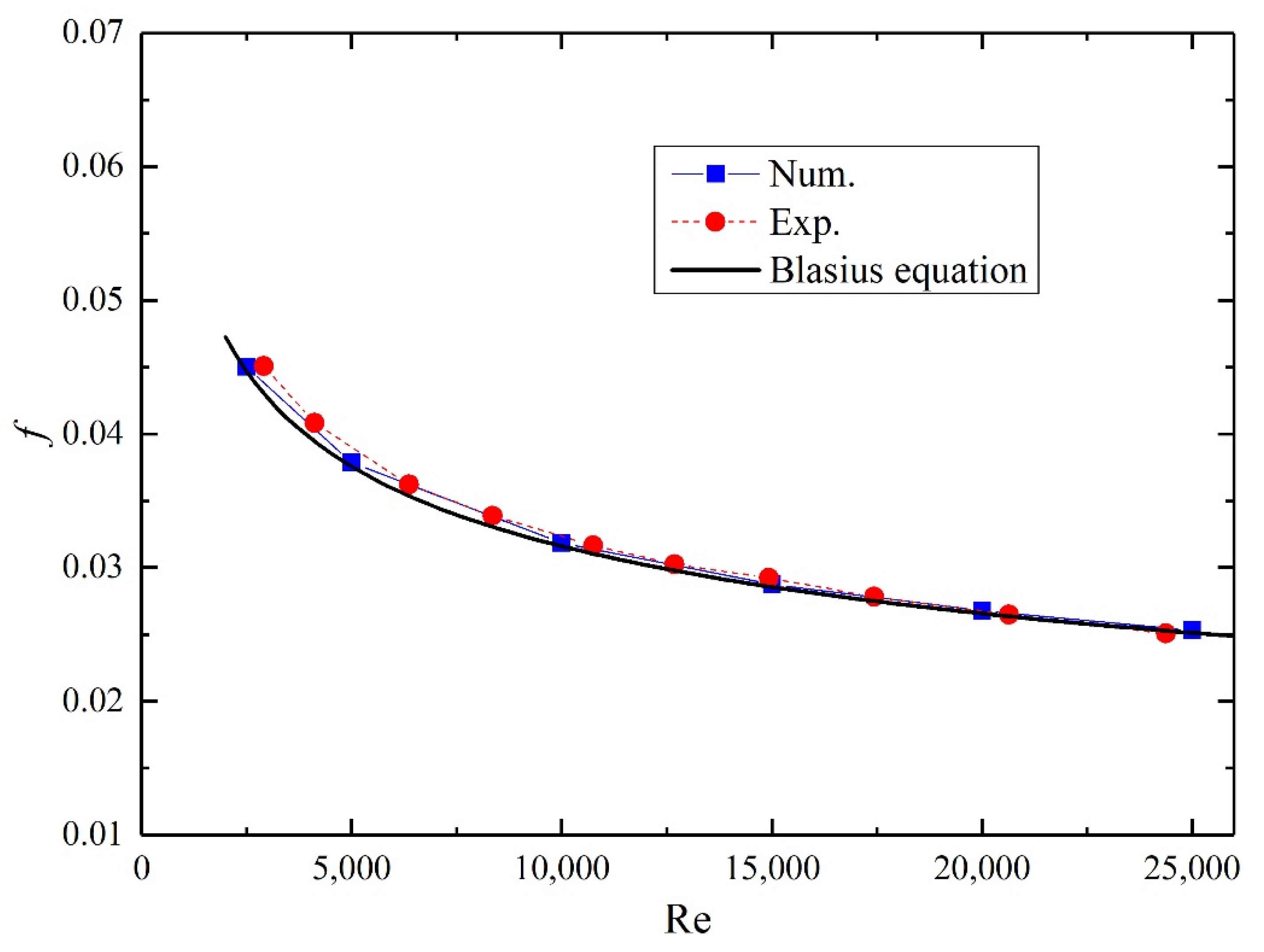
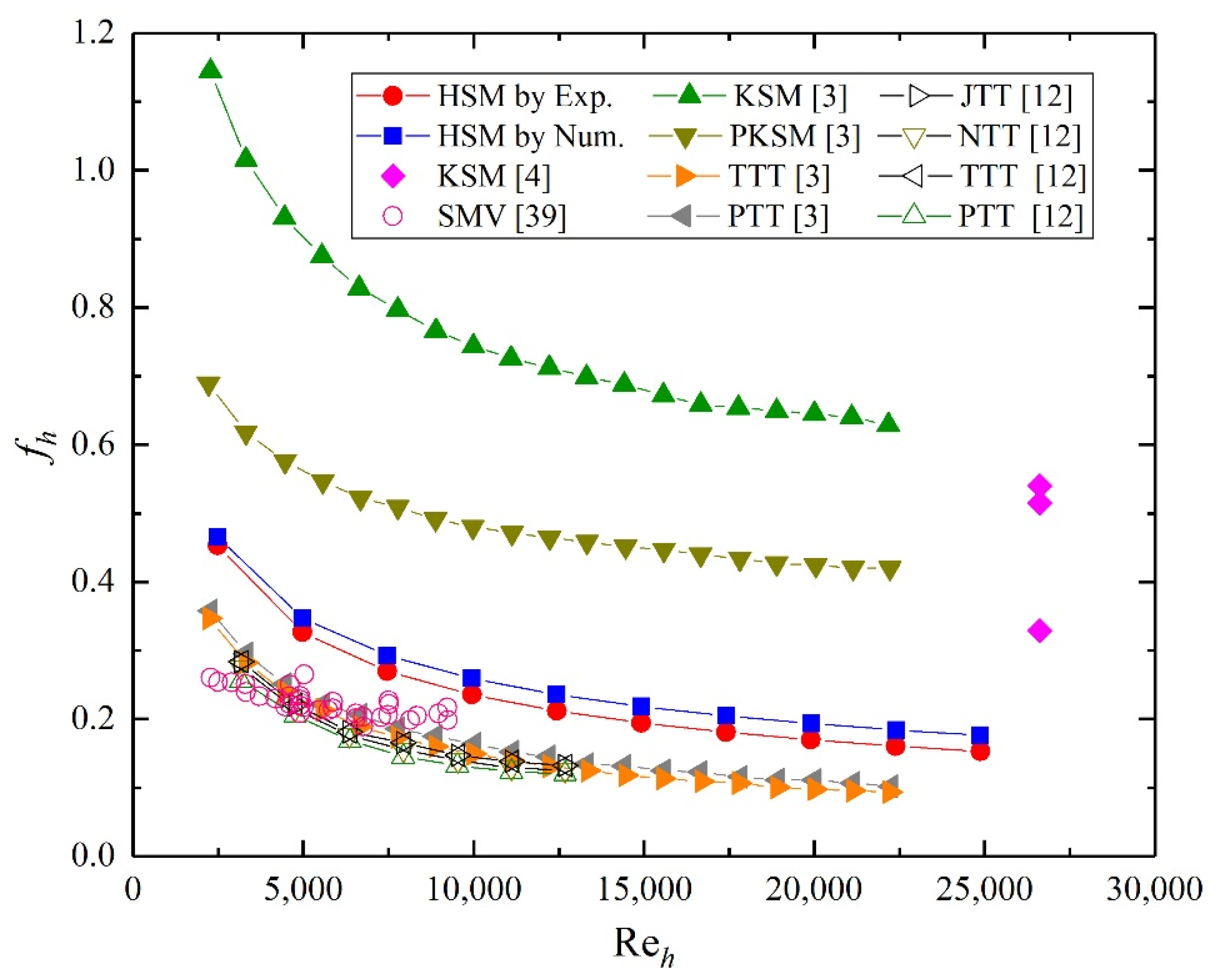
4.2.1. Comparison of the Friction Factors

The flow resistance in a static mixer can be evaluated by the modified friction factor f_h considering the geometric characteristics of static mixer [50]:

$$f_h=\frac{\mathsf{\Delta }P{\epsilon }^2}{2{\rho }_l{V}_0^2(L/D_h)}$$

(11)

where ε is the porosity, D_h is the hydraulic diameter which equals the difference of the outer diameter and the inner diameter (D_o − D_i). The modified Reynolds number is defined as Re_h = ρ_lV₀D_h/(εμ_l). The Reynolds numbers referred to below are all Re_h. Although no baffles are added in the pipeline with HSM, a change in the flow structure can also increase the pressure drop of fluid flow. Friction factors of fluid flow in the static mixers varying with the Reynolds number are presented in Figure 7. The results given by the current study is shown in solid dots, and the data reported by Meng et al. [3], Rabha et al. [4], Lobry et al. [39], and Rahimi et al. [12] are shown in hollow dots for comparison.

The friction factor of fluid flow with HSM decreases with the augment of the Reynolds number. f_h drops quickly at the low-Re region and tends to unchanged when the Reynolds number is high. The numerical results are slightly larger than the experimental data, which may be attributed to the drag reduction effect of bubbly flow [51]. The results are much better than those of KSM and PKSM, which are designed with staggered mixing elements. The perforated holes on the PKSM weaken the turbulence of the flow stream and reduce the flow resistance of the KSM. All of the static mixers with a continuous helical structure give lower friction factors than the KSM. Friction factors of the HSM are slightly larger than those of PTT, TTT, JTT, NTT, and SMV. The PTT, TTT, JTT, and NTT are twisted tapes with smooth surfaces, hence, the flow structure is steady along the continuous helical flow channel. Besides, the existence of slip velocity between the gas and the liquid at the entrance enlarges the flow resistance of the HSM. Four pairs of side surfaces of the flow channels in the HSM are rough with small steps, which makes the friction factors of the HSM relatively large. The SMV gives small friction factors that may be attributed to the high dispersed phase concentration (φ = 25%) studied by Lobry et al. [39].

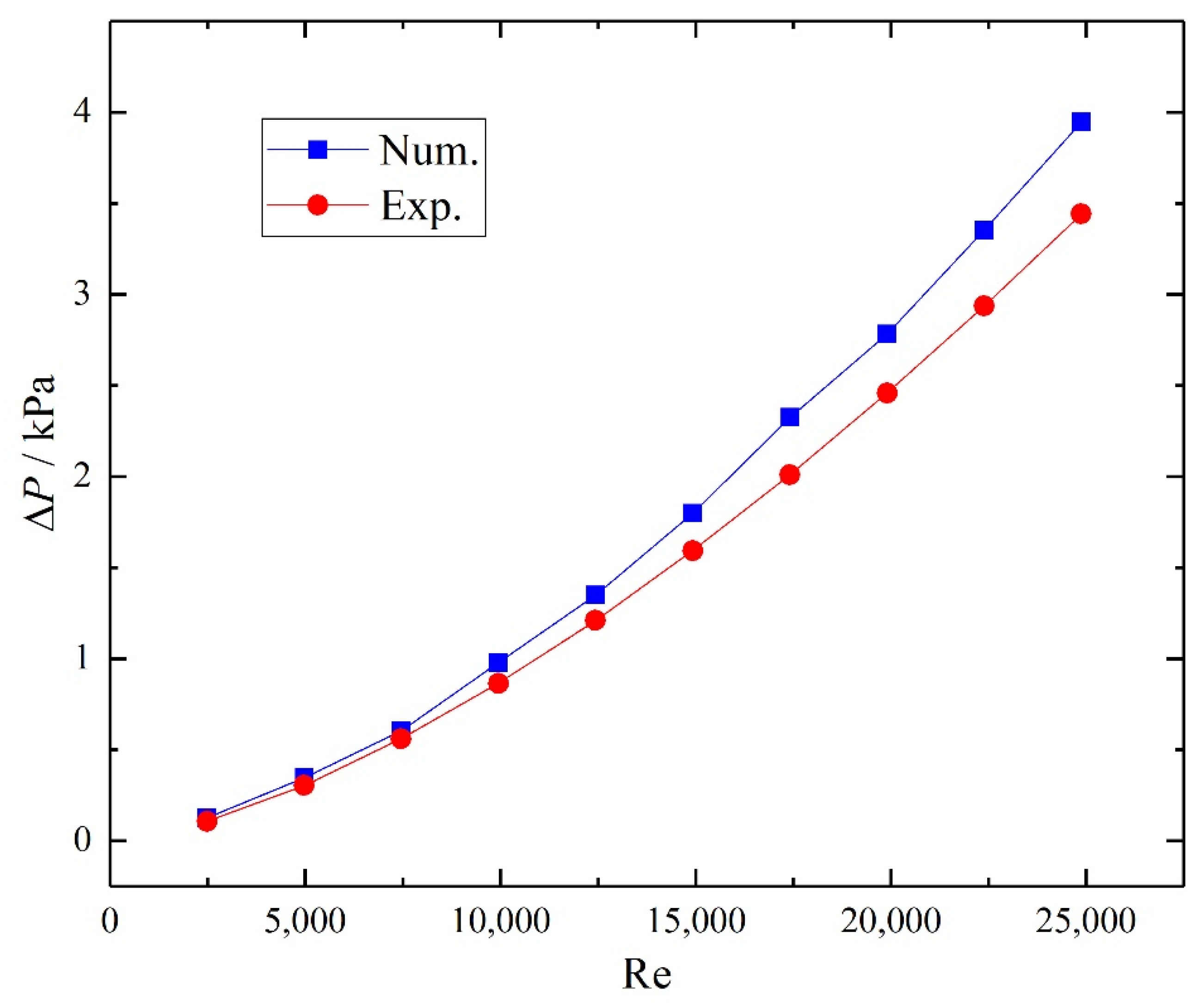
4.2.2. Effect of the Reynolds Number

A large pressure drop stands for high energy expenditure in applications. Figure 8 gives the total pressure drop ΔP of fluid flow through the HSM at different Reynolds numbers. The curves for numerical and experimental results show similar trends. The pressure drop increases with the Reynolds number, and the increment is larger when the Reynolds number is higher. The numerical results are larger than the experimental data because of the velocity difference between the fluid and the gas flow. At the entrance, the gas–liquid velocity difference increases with the argument of the Reynolds number. Hence, the pressure drop of fluid flow at the front stage becomes larger, as seen in Figure 9. So, the inlet boundary condition may contribute to the difference between the two curves in Figure 8.

The pressure drop along the HSM varies because of the variable helical pitch structure. The equidistant pressure drops indicate the effect of variable pitch on flow resistance. Here, the equidistant pressure drop between two adjacent sections separated by 40 mm is defined as:

$$\delta P=P_z-P_{z-40}$$

(12)

where z is the distance from the HSM inlet (mixing length). Figure 9 gives the δP along the axial distance at different Reynolds numbers when m = 0.5. The pressure at different cross-sections inside the HSM is hard to measure, so the data in this figure is obtained by numerical simulations. The entrance effect mentioned above leads to large pressure drops from inlet to z = 80 mm. As the flow develops, the pressure drop increases as the helical pitch decreases. The equidistant pressure drop increases with the argument of Reynolds number, and increases when the pitch decreases from upstream to downstream. The effect of the variable pitch is invisible in the low-Re region (Re < 5000).

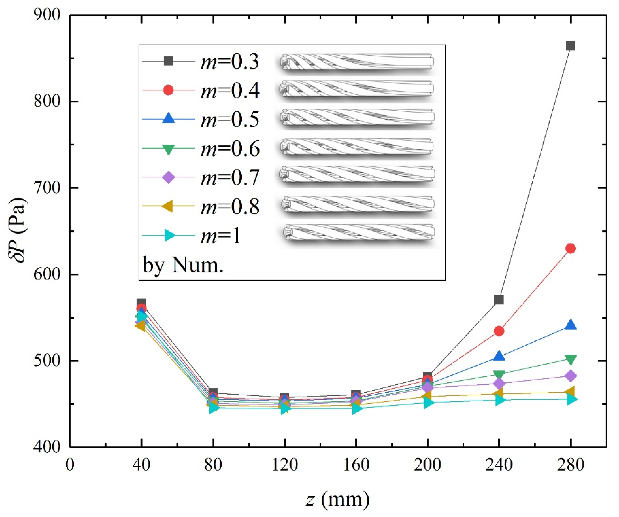
4.2.3. Effect of the Variable-Pitch Coefficient

Figure 10 gives the equidistant pressure drop at different flow distances at Re = 22,392. The entrance effect appears as well. The equidistant pressure drop is slightly larger when the variable-pitch coefficient is smaller. After half-length of the flow distance in the HSM (z > 140 mm), the δP increases quickly, and highly affected by the variable-pitch coefficient. The equidistant pressure drop increases significantly when the variable-pitch coefficient m < 0.5. When m is smaller, the flow channel is more twisted. Hence, the axial velocity of fluid flow transfers to circumferential helical velocity. The flow resistance increases per unit flow distance with more viscous dissipation. So, the energy expenditure will significantly increase if the variable-pitch coefficient is too small.

4.3. Bubble Transport

4.3.1. Change of the BSD

For numerical simulations, the parameters that describe BSD are given by:

$$\begin{array}{l}N=m_0\\ v_g=\frac{m_1^2}{m_0^{3/2}{m}_2^{1/2}}\\ l{n}^2{\sigma }_g=\frac{1}{9}ln(\frac{m_0{m}_2}{m_1^2})\end{array}$$

(13)

where N denotes the total number of bubbles per unit volume. Equation (13) is used to obtain the BSD which is assumed to be the log-normal distribution. The average bubble diameter d₃₂ can be determined by the zeroth- and first-order moments: d₃₂ = (6/π·m₁/ m₂)^1/3 [38].

The probability density function (PDF) of bubble sizes at the inlet and the outlet are presented in Figure 11. The measured average BSD at the inlet is fitted as a log-normal distribution, of which the bubble geometric mean diameter (GMD) is 477.6μm and GSD is 1.256. The outlet GMD and GSD are 7.3 μm and 1.644, respectively. The numerical results reveal that the GMD of bubbles reduces to 4.48 μm and the GSD of the bubble population increases to 1.384 after the fluid flow through the HSM. The BSD of experimental results is more uniform than that of numerical simulations and the GMD is larger. Rabha et al. [4] listed the available correlations for predicting the bubble size in HSM. Most of the formulas are used for liquid–liquid conditions. Although the equations for dispersed gas and liquid are identical for pipeline flows [1], the classical models are not fit for the current study. The main reason is that the bubbles at the inlet are generated by a venturi nozzle. The air phase is dispersed through two stages to microbubbles. In fact, the correlation for bubble size is hard to be determined under different dimensions and conditions. Besides, data for the comparison of bubble size are hard to find in the literature [4]. In this study, only the effects of Reynolds number and variable-pitch coefficient are discussed, and no correlations are given.

The breakup of bubbles in the HSM is mainly induced by an adequate shear rate near the serial steps. Due to the helical structure of the mixer, the bubble population runs into one side of the flow channel after entering the device. The surface of both sides of the flow channel is similar to the traditional washboard, which consists of a series of ridges or corrugations. The continuous step structure formed by the staggered steel sheets induces strong flow separation [52] and turbulence. The local shear rate is far larger near the steps than the central flow region. Hence, the bubbles break into smaller bubbles under the adequate hydrodynamic shearing. The number of bubbles and the GSD increase after the fluid passes through the flow path. With the development of fluid flow, the bubbles migrate across the central region to the other side of the flow channel, where the hydrodynamic shearing keeps breaking the bubbles into small sizes.

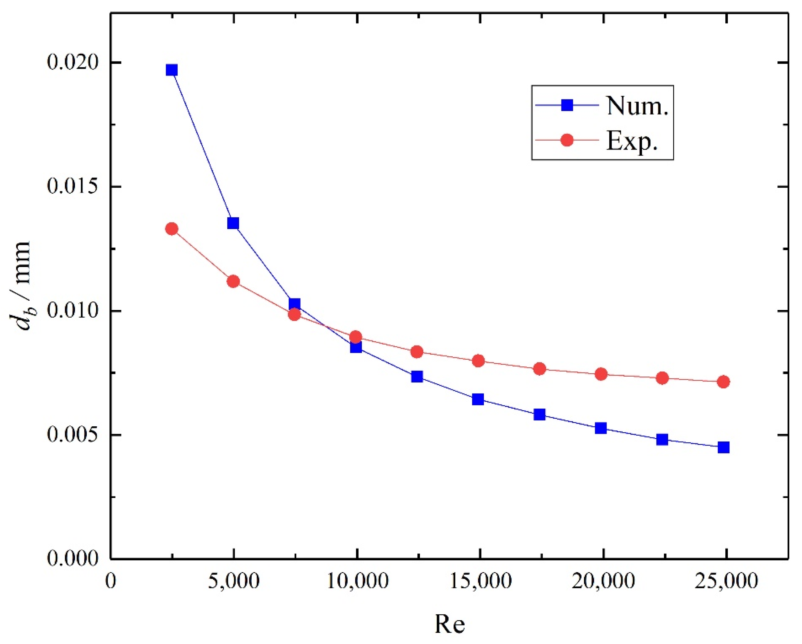
4.3.2. Effect of the Reynolds Number

Figure 12 gives the GMD of bubbles at the outlet with different Reynolds numbers. The numerical and experimental results show a similar trend that is the bubble diameter in the suspensions decreases with the argument of Reynolds number. The rate of change of bubble size is larger for the numerical prediction than the experimental measurement. In the low-Re region, the bubble size given by numerical simulations is larger. In contrast, experiments give a larger bubble size in suspensions when Re is larger than 10,000. The results agree with the picture of microbubbles in Figure 4. The change of the bubble GMD decreases with the argument of the Reynolds number, which reveals that the HSM may be hard to break up bubbles into smaller sizes. That is to say, the effect of the HSM has a limitation on breaking the bubbles less than a certain size.

The average bubble diameters along the axial distance at different Reynolds numbers are shown in Figure 13. The GMD of bubbles decreases at different cross-sections along the flow direction. The gas flow rate is constant and the increase of liquid flow rate leads to the argument of Re, so the gas holdup decreases when Re increases. The inlet bubble GMD decreases with the increase of the bulk velocity and the decrease of the gas holdup. The inlet bubble GMDs range from 0.11 to 0.89 mm when the Reynolds number varies from 2488 to 24,880. Although the sampled data are plotted by a logarithmic coordinate, the drop of the curves becomes faster when the fluid flows towards downstream. The trend may be caused by the effect of the variable pitch structure. The entrance effect is invisible to the bubble size.

4.3.3. Effect of the Variable-Pitch Coefficient

Figure 14 gives the GMD along the axial distance at Re = 22,392. All of the curves drop with different variable-pitch coefficients ranging from 0.3 to 1. The HSM with m = 1 means that the pitch is constant. The bubble can be broken into microbubbles with a diameter of about 1 μm at m = 0.3. The change of the bubble size is up to 96% when m changes from 1 to 0.3. The bubble GMD decreases significantly when the variable-pitch coefficient becomes smaller. The design of the variable pitch enhances the bubble breakup effectively. However, the decrease in the variable-pitch coefficient brings about the increase of energy expenditure. So, the design of HSM with a moderate variable-pitch coefficient is reasonable for industrial applications.

5. Conclusions

In conclusion, the flow resistance and bubble transport in a new type of helical static mixer were studied experimentally and numerically. The inline mixer increases the volume fraction of gas in liquids by breaking bubbles into smaller sizes with a micrometer size in the flow experiments. The gas–liquid flow was simulated by a combination of computational fluid dynamics and Taylor expansion methods of moments.

The friction factor of the helical static mixer is smaller than that of the KSM and the PKSM, but larger than that of the TTT and the PTT. The pressure drop increases with the Reynolds number, and the increment is larger when the Reynolds number is higher. The equidistant pressure drop increases with the argument of Reynolds number, and increases when the pitch decreases from upstream to downstream. The energy expenditure increases significantly when the variable-pitch coefficient is too small.

The bubble geometric mean diameter decreases, and the geometric standard deviation increases when the gas–liquid fluid flows through the mixer. The variable pitch structure enhances the bubble breakup effectively. The change of the bubble GMD decreases with the argument of the Reynolds number. The effect of the HSM has a limitation on breaking the bubbles.

The device is motionless, low energy-consumption, easy to manufacture, low-cost and has low requirements for medium. It is a high-quality equipment for mixing and mass transfer, and can be widely used in industries. Further investigations performed on the helical static mixer would optimize the design of equipment and numerical model, and the effects of the helix line equation and the pressure on bubble size distribution will be discussed in the future.

References

1. Paul, E.L.; Atiemo-Obeng, V.A.; Kresta, S.M. Handbook of Industrial Mixing: Science and Practice; Wiley & Sons: Hoboken, NJ, USA, 2004. [Google Scholar] [CrossRef]
2. Malecha, Z.M.; Malecha, K. Numerical analysis of mixing under low and high frequency pulsations at serpentine micromixers. Chem. Process. Eng. 2014, 35, 369–385. [Google Scholar] [CrossRef]
3. Meng, H.; Zhu, G.; Yu, Y.; Wang, Z.; Wu, J. The effect of symmetrical perforated holes on the turbulent heat transfer in the static mixer with modified Kenics segments. Int. J. Heat Mass Transf. 2016, 99, 647–659. [Google Scholar] [CrossRef]
4. Rabha, S.; Schubert, M.; Grugel, F.; Banowski, M.; Hampel, U. Visualization and quantitative analysis of dispersive mixing by a helical static mixer in upward co-current gas–liquid flow. Chem. Eng. J. 2015, 262, 527–540. [Google Scholar] [CrossRef]
5. Park, J.M.; Kim, D.S.; Kang, T.G.; Kwon, T.H. Improved serpentine laminating micromixer with enhanced local advection. Microfluid. Nanofluid. 2008, 4, 513–523. [Google Scholar] [CrossRef]
6. Stroock, A.D.; Dertinger, S.K.W.; Ajdari, A.; Mezić, I.; Stone, H.A.; Whitesides, G.M. Chaotic mixer for microchannels. Science 2002, 295, 647–651. [Google Scholar] [CrossRef] [Green Version]
7. Zhang, C.; Ferrell, A.R.; Nandakumar, K. Study of a toroidal-helical pipe as an innovative static mixer in laminar flows. Chem. Eng. J. 2019, 359, 446–458. [Google Scholar] [CrossRef]
8. Ghanem, A.; Lemenand, T.; Della Valle, D.; Peerhossaini, H. Static mixers: Mechanisms, applications, and characterization methods-a review. Chem. Eng. Res. Des. 2014, 92, 205–228. [Google Scholar] [CrossRef]
9. Hobbs, D.; Muzzio, F. The Kenics static mixer: A three-dimensional chaotic flow. Chem. Eng. J. 1997, 67, 153–166. [Google Scholar] [CrossRef]
10. Putra, R.A.; Neumann-Kipping, M.; Schäfer, T.; Lucas, D. Comparison of gas–liquid flow characteristics in geometrically different swirl generating devices. Energies 2019, 12, 4653. [Google Scholar] [CrossRef] [Green Version]
11. Lei, Y.G.; Zhao, C.H.; Song, C.F. Enhancement of turbulent flow heat transfer in a tube with modified twisted tapes. Chem. Eng. Technol. 2012, 35, 2133–2139. [Google Scholar] [CrossRef]
12. Rahimi, M.; Shabanian, S.R.; Alsairafi, A.A. Experimental and CFD studies on heat transfer and friction factor characteristics of a tube equipped with modified twisted tape inserts. Chem. Process. Eng. 2009, 48, 762–770. [Google Scholar] [CrossRef]
13. Cui, Y.-Z.; Tian, M.-C. Three-dimensional numerical simulation of thermal-hydraulic performance of a circular tube with edgefold-twisted-tape inserts. J. Hydrodyn. Ser. B 2010, 22, 662–670. [Google Scholar] [CrossRef]
14. Cerezo, J.; Best, R.; Chan, J.J.; Romero, R.J.; Hernandez, J.I.; Lara, F. A theoretical-experimental comparison of an improved ammonia-water bubble absorber by means of a helical static mixer. Energies 2017, 11, 56. [Google Scholar] [CrossRef] [Green Version]
15. Thianpong, C.; Eiamsa-ard, P.; Eiamsa-ard, S. Heat transfer and thermal performance characteristics of heat exchanger tube fitted with perforated twisted-tapes. Heat Mass Transf. 2012, 48, 881–892. [Google Scholar] [CrossRef]
16. Eiamsa-ard, S.; Nuntadusit, C.; Promvonge, P. Effect of twin delta-winged twisted-tape on thermal performance of heat exchanger tube. Heat Transf. Eng. 2013, 34, 1278–1288. [Google Scholar] [CrossRef]
17. Zidouni, F.; Krepper, E.; Rzehak, R.; Rabha, S.; Schubert, M.; Hampel, U. Simulation of gas–liquid flow in a helical static mixer. Chem. Eng. Sci. 2015, 137, 476–486. [Google Scholar] [CrossRef]
18. Ushikubo, F.Y.; Furukawa, T.; Nakagawa, R.; Enari, M.; Makino, Y.; Kawagoe, Y.; Shiina, T.; Oshita, S. Evidence of the existence and the stability of nano-bubbles in water. Colloids Surf. Phys. Eng. Asp. 2010, 361, 31–37. [Google Scholar] [CrossRef]
19. Turner, W.R. Microbubble persistence in fresh water. J. Acoust. Soc. Am. 1961, 33, 1223. [Google Scholar] [CrossRef]
20. Lawrie, A.; Brisken, A.F.; Francis, S.E.; Cumberland, D.C.; Crossman, D.C.; Newman, C.M. Microbubble-enhanced ultrasound for vascular gene delivery. Genetherapy 2000, 7, 2023. [Google Scholar] [CrossRef] [Green Version]
21. Sakai, O.; Kimura, M.; Shirafuji, T.; Tachibana, K. Underwater microdischarge in arranged microbubbles produced by electrolysis in electrolyte solution using fabric-type electrode. Appl. Phys. Lett. 2008, 93, 3. [Google Scholar] [CrossRef] [Green Version]
22. Sadatomi, M.; Kawahara, A.; Matsuura, H.; Shikatani, S. Micro-bubble generation rate and bubble dissolution rate into water by a simple multi-fluid mixer with orifice and porous tube. Exp. Therm. Fluid Sci. 2012, 41, 23–30. [Google Scholar] [CrossRef]
23. Heyouni, A.; Roustan, M.; Do-Quang, Z. Hydrodynamics and mass transfer in gas–liquid flow through static mixers. Chem. Eng. Sci. 2002, 57, 3325–3333. [Google Scholar] [CrossRef]
24. Putra, R.A.; Schäfer, T.; Neumann, M.; Lucas, D. CFD studies on the gas–liquid flow in the swirl generating device. Nucl. Eng. Des. 2018, 332, 213–225. [Google Scholar] [CrossRef]
25. Cong, T.; Zhang, X. Numerical study of bubble coalescence and breakup in the reactor fuel channel with a vaned grid. Energies 2018, 11, 256. [Google Scholar] [CrossRef] [Green Version]
26. Falzone, S.; Buffo, A.; Vanni, M.; Marchisio, D.L. Simulation of Turbulent Coalescence and Breakage of Bubbles and Droplets in the Presence of Surfactants, Salts, and Contaminants. Adv. Chem. Eng. 2018, 52, 125–188. [Google Scholar] [CrossRef]
27. Martinez, C.; Rodriguez, J.; Deane, G.; Montañes, J.; Lasheras, J. Considerations on bubble fragmentation models. J. Fluid Mech. 2010, 661, 159–177. [Google Scholar] [CrossRef] [Green Version]
28. Tran-Cong, S.; Marié, J.-L.; Perkins, R.J. Bubble migration in a turbulent boundary layer. Int. J. Multiph. Flow 2008, 34, 786–807. [Google Scholar] [CrossRef]
29. Azizi, F.; Al Taweel, A. Population balance simulation of gas–liquid contacting. Chem. Eng. Sci. 2007, 62, 7436–7445. [Google Scholar] [CrossRef]
30. Coulaloglou, C.; Tavlarides, L. Description of interaction processes in agitated liquid-liquid dispersions. Chem. Eng. Sci. 1977, 32, 1289–1297. [Google Scholar] [CrossRef]
31. Vyakaranam, K.V.; Kokini, J.L. Prediction of air bubble dispersion in a viscous fluid in a twin-screw continuous mixer using FEM simulations of dispersive mixing. Chem. Eng. Sci. 2012, 84, 303–314. [Google Scholar] [CrossRef]
32. Nguyen, V.T.; Song, C.-H.; Bae, B.-U.; Euh, D.-J. Modeling of bubble coalescence and break-up considering turbulent suppression phenomena in bubbly two-phase flow. Int. J. Multiph. Flow 2013, 54, 31–42. [Google Scholar] [CrossRef]
33. Chouippe, A.; Climent, E.; Legendre, D.; Gabillet, C. Numerical simulation of bubble dispersion in turbulent Taylor-Couette flow. Phys. Fluids 2014, 26, 043304. [Google Scholar] [CrossRef]
34. Mukin, R. Modeling of bubble coalescence and break-up in turbulent bubbly flow. Int. J. Multiph. Flow 2014, 62, 52–66. [Google Scholar] [CrossRef]
35. Liao, Y.; Rzehak, R.; Lucas, D.; Krepper, E. Baseline closure model for dispersed bubbly flow: Bubble coalescence and breakup. Chem. Eng. Sci. 2015, 122, 336–349. [Google Scholar] [CrossRef]
36. Kumar, S.; Ramkrishna, D. On the solution of population balance equations by discretization-I. A fixed pivot technique. Chem. Eng. Sci. 1996, 51, 1311–1332. [Google Scholar] [CrossRef]
37. Asiagbe, K.S.; Fairweather, M.; Njobuenwu, D.O.; Colombo, M. Large eddy simulation of microbubble transport in a turbulent horizontal channel flow. Int. J. Multiph. Flow 2017, 94, 80–93. [Google Scholar] [CrossRef] [Green Version]
38. Jaworski, Z.; Pianko-Oprych, P.; Marchisio, D.L.; Nienow, A.W. CFD modelling of turbulent drop breakage in a Kenics static mixer and comparison with experimental data. Chem. Eng. Res. Des. 2007, 85, 753–759. [Google Scholar] [CrossRef]
39. Lobry, E.; Theron, F.; Gourdon, C.; Le Sauze, N.; Xuereb, C.; Lasuye, T. Turbulent liquid-liquid dispersion in SMV static mixer at high dispersed phase concentration. Chem. Eng. Sci. 2011, 66, 5762–5774. [Google Scholar] [CrossRef] [Green Version]
40. Lebaz, N.; Sheibat-Othman, N. A population balance model for the prediction of breakage of emulsion droplets in SMX+ static mixers. Chem. Eng. J. 2019, 361, 625–634. [Google Scholar] [CrossRef]
41. Arffman, A.; Marjamäki, M.; Keskinen, J. Simulation of low pressure impactor collection efficiency curves. J. Aerosol Sci. 2011, 42, 329–340. [Google Scholar] [CrossRef]
42. Liao, Y.; Lucas, D. A literature review of theoretical models for drop and bubble breakup in turbulent dispersions. Chem. Eng. Sci. 2009, 64, 3389–3406. [Google Scholar] [CrossRef]
43. Saffman, P.; Turner, J. On the collision of drops in turbulent clouds. J. Fluid Mech. 1956, 1, 16–30. [Google Scholar] [CrossRef] [Green Version]
44. Qin, C.; Yang, N. Population balance modeling of breakage and coalescence of dispersed bubbles or droplets in multiphase systems. Prog. Chem. 2016, 28, 1207–1223. [Google Scholar] [CrossRef]
45. Barthelmes, G.; Pratsinis, S.; Buggisch, H. Particle size distributions and viscosity of suspensions undergoing shear-induced coagulation and fragmentation. Chem. Eng. Sci. 2003, 58, 2893–2902. [Google Scholar] [CrossRef]
46. Yu, M.; Lin, J.; Chan, T. A new moment method for solving the coagulation equation for particles in Brownian motion. Aerosol Sci. Technol. 2008, 42, 705–713. [Google Scholar] [CrossRef]
47. Chan, T.L.; Liu, S.; Yue, Y. Nanoparticle formation and growth in turbulent flows using the bimodal TEMOM. Powder Technol. 2018, 323, 507–517. [Google Scholar] [CrossRef]
48. Yu, P.; Jiang, J.; Cheng, K. Preparation of oxygen-enriched water by spiral cutter and its process optimization. Light Ind. Mach. 2018, 36, 41–47. [Google Scholar] [CrossRef]
49. Zhi-qing, W. Study on correction coefficients of liminar and turbulent entrance region effect in round pipe. Appl. Math. Mech. Engl. 1982, 3, 433–446. [Google Scholar] [CrossRef]
50. Theron, F.; Sauze, N.L. Comparison between three static mixers for emulsification in turbulent flow. Int. J. Multiph. Flow 2011, 37, 488–500. [Google Scholar] [CrossRef] [Green Version]
51. Sugiyama, K.; Calzavarini, E.; Lohse, D. Microbubbly drag reduction in Taylor-Couette flow in the wavy vortex regime. J. Fluid Mech. 2008, 608, 21–41. [Google Scholar] [CrossRef] [Green Version]
52. Chen, L.; Asai, K.; Nonomura, T.; Xi, G.; Liu, T. A review of backward-facing step (BFS) flow mechanisms, heat transfer and control. Therm. Sci. Eng. Prog. 2018, 6, 194–216. [Google Scholar] [CrossRef]
Figure 1. The configuration of static mixing elements with helical structure.
Energies 13 01228 g001
Figure 2. Schematic diagram of the static mixing internals.
Energies 13 01228 g002
Figure 3. Schematic of the experimental setup (1—centrifugal pump; 2—flow control valve; 3—liquid flow meter; 4—venturi bubble generator; 5—pressure gauge; 6—helical static mixer; 7—pressure gauge; 8—storage tank; 9—Laser Analyzer; 10—Computer; 11—exhaust gas treatment; 12—control box; 13—gas cylinder; 14—gas release control valve; 15—gas flow meter).
Energies 13 01228 g003
Figure 4. Microscope picture of microbubbles dispersed in water.
Energies 13 01228 g004
Figure 5. Computational domain and mesh.
Energies 13 01228 g005
Figure 6. Comparison of the friction factors of turbulent open pipe flows.
Energies 13 01228 g006
Figure 7. Friction factor versus Reynolds number.
Energies 13 01228 g007
Figure 8. Total pressure drop along the HSM.
Energies 13 01228 g008
Figure 9. Equidistant pressure drop along the axial distance at different Reynolds numbers (m = 0.5).
Energies 13 01228 g009
Figure 10. Equidistant pressure drop versus flow distance with different m.
Energies 13 01228 g010
Figure 11. PDF of bubble sizes at the inlet and the outlet (m = 0.5).
Energies 13 01228 g011
Figure 12. GMD of bubbles at the outlet (m = 0.5).
Energies 13 01228 g012
Figure 13. Average bubble diameter along the axial distance at different Reynolds numbers (m = 0.5).
Energies 13 01228 g013
Figure 14. Average bubble diameter along the axial distance with different m.
Energies 13 01228 g014