Mathematical Modelling of Drive System with an Elastic Coupling Based on Formal Analogy between the Transmission Shaft and the Electric Transmission Line

Abstract

In the paper, the kinematic structure of the transmission shaft between the driving motor and the working mechanism is studied. The analysis is based on electrical and mechanical similarities. The equivalent circuits, typical for electrical systems, are defined for the transmission shaft concerned. Modelling of the transmission shaft based on a formal analogy between the transmission shaft and the electric transmission line is also proposed. The results of a computer simulation and experimental test are presented. The results confirm the high conformity of the proposed mathematical model with the physical object.

1. Introduction

Rapid development and diversity of electric drive systems require extensive theoretical and practical knowledge as well as the use of a wide range of theoretical and constructional solutions from the contemporary designers and users. Electric drive systems are used in all branches of industry; therefore, the trouble-free operation of these systems is of crucial importance. An analysis of the states of electric drive operation is often related to ensuring its safety. A key issue is to detect the mechanical resonance phenomenon or the phenomena close to resonance as the most unsafe ones for the system. Ignoring the analysis and the ongoing diagnostics of vibrations in electromechanical systems results in many failures. The example, including fatalities, is inter alia the failure of turbo generator set in the power plant Kostromska (Russia). In the commission view, the cause of the failure was ignoring torsional vibrations, which led to the resonance in the turbine and transmission shaft included in the turbo-generator set.

A very interesting case of the electric submersible pumps system with a multi-component system powered by a soft start system is shown in [1]. In this real case scenario, the incorrect control case led to resonance phenomena and a shaft breakdown. Therefore, comprehensive research is needed to analyse the operating states of electrical and electromechanical systems. One method to investigate the dynamic behaviour of electrical and electromechanical systems is an experimental test directly on the system. In many cases, the experimental tests on the system are not possible, due to technical reasons, costs of experiments or their duration. The alternative approach to the investigation into the system behaviour is the formulation of the model and carrying out the investigations into the model. The model of a system is the representation using mathematical relationships, a physical model or an analogue model. The physical model of the real-world system includes smaller-scale components having the same physical nature as a real-world system. In the physical model, there are phenomena described by the same dependencies, differing only in the order of magnitude. The analogue model includes components having a different physical nature than the real-world system, but these components are easier to implement. The analogue models are based on physical analogy. An electrical circuit may be defined as the analogue model of the mechanical system. The mathematical model is the set of mathematical relationships, on the basis of which the behaviour of a system can be predicted. The mathematical model is most often formulated as differential equations describing the operation of a system. Each physical model has a corresponding mathematical model.

The mathematical model of a mechanical object is usually a set of partial differential equations. They are hard to solve both analytically and numerically. Discrete models of systems include ordinary differential equations; therefore, they are used in practice most often. Real-world mechanical systems are usually nonlinear, where the nonlinearity is determined by material properties, clearances, nonlinear nature of dissipation forces and characteristics of elastic elements. A limited possibility of analysis of nonlinear differential equations leads towards the use of linear models or the linearization of those. There are a lot of physical systems, which may be represented by linear models with accuracy acceptable for practice. In the process of creating the models of physical systems, the equations of motion are formulated.

An electric motor, being part of an electric drive, is coupled with a working mechanism via a driving shaft that is an element of mechanical power transmission. Mechanical power transmissions can be a single-path or a multi-path and can also include gear trains and clutches [2]. The long driving shafts, defined as transmission shafts, are used first of all in the drive systems for the steel industry, mainly in the drive systems for rolling mills—the transmission shafts are over 10 m long and their diameters are of 0.5 to 0.8 m. Transmission shafts are also used in drive systems for polymerization reactors. The length of these shafts is from 4 to 7 m. Moreover, transmission shafts are used in hydro generator sets, ship drive systems, submarine drive systems, etc. Depending on the length and cross-section, transmission shafts can demonstrate different susceptibilities to the impact of the moment of torsion, as measured by a value of the angle of twist [2]. In the case of short mechanical coupling, the value of the angle of twist is insignificant and may be omitted by the assumption of rigid mechanical coupling, whereas in the case of longer mechanical coupling the value of the angle of twist cannot be ignored and such coupling should be considered as the elastic one [1,2,3,4,5,6,7,8,9,10].

In order to model the transmission shaft, classical methods based on the d’Alembert principle or Newton’s second law as well as the variational method are used. The use of the variational method results in the distributed parameter model consisting of partial differential equations [3]. An example of a partial differential equation used to describe a long elastic element is the wave equation [11]. Partial differential equations may be solved analytically, but this is both tedious and time-consuming. Thus, these equations are usually transformed into ordinary differential equations by using finite differences [2]. The model of the long elastic element, based on the ordinary differential equations, corresponds with a multi-mass lumped parameter model, e.g., in [2,12,13], especially the two-mass model, e.g., in [6,8,14], which does not guarantee the accurate results of numerical analysis. The equations included in the multi-mass model are usually solved using numerical integration.

Research on stresses and oscillations of long drive shafts using various methods of analysis is undertaken in the literature [15,16,17,18]. In [18], the author presents a mechanical analysis of the propeller shaft on a warship in the event of a variable moment of shaft load. Modelling of the object is selected on a classic approach using a system of nonlinear equations. A similar approach, but using a different model and a different scale, with a three-mass system, is shown in [16]. The author shows comparative results between the analytical calculations of the two-mass system and the numerical calculations for the three-mass system. An extended approach to analysing the issue of three-mass and two-mass system including changes in the moment of inertia is shown in [18]. In all of the above described publications, the authors used a classical approach in different variations.

In this paper, the kinematic structure of the transmission shaft between the driving motor and the working mechanism was studied. The telegrapher’s equations and their d’Alembert solution are proposed for the mathematical description of the transmission shaft. The proposed modelling is an alternative to the multi-mass model based on ordinary differential equations as well as a distributed parameter model based on partial differential equations. The advantage of the proposed model is its simplicity, due to the fact that the model is based on discrete equations, which do not require numerical integration in contrast to the models based on differential equations. The presented modelling is based on electrical and mechanical similarities. Identifying these similarities is very helpful for electricians in finding a relevant interpretation of mechanical systems, which is particularly important in the case of professionals dealing with electromechanical energy converters or drive systems [2]. The aim of the presented study was to achieve very high conformity of the mathematical model with the physical object, whilst keeping a short time for numerical calculations.

2. Methods of Modelling of Transmission Shaft on the basis of Electrical and Mechanical Similarities

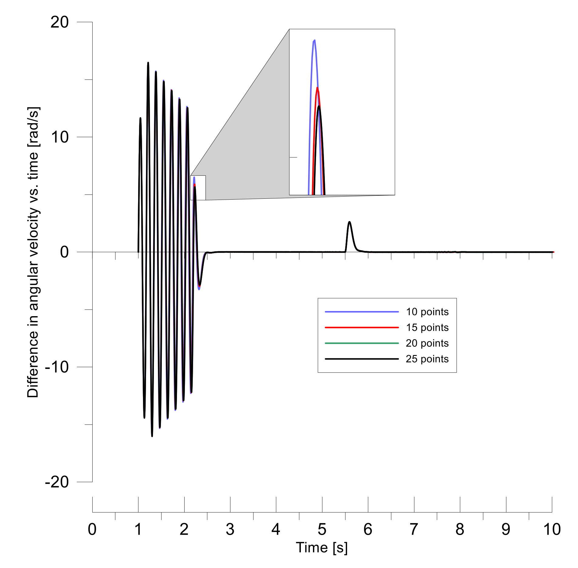
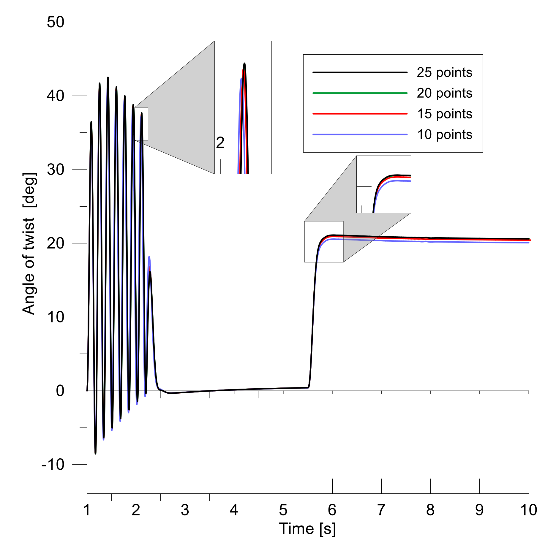
The mass of the real transmission shaft (or any element) is distributed continuously. Representing such a transmission shaft by a model based on lumped parameters causes discrepancies in the results of the analysis in relation to accurate models. These discrepancies decrease with the number of points of concentration in the model. Dividing a transmission shaft with distributed mass into several shorter elements, described by lumped parameters such as mass, elasticity and damping of the i-th element, it is possible to obtain the results of computer simulation essentially not different from the results obtained if the shaft is divided into infinite number of elements, that corresponds with the wave model. The process of the abovementioned division is referred to as discretization of kinematic structure and corresponds with the multi-mass lumped parameter model of the transmission shaft.

In order to present the synthesis of the proposed models of the transmission shaft, the following assumptions have been adopted:

-

transmission shaft is the elastic element,

-

in the case of the lumped parameter model, the shaft is divided into a finite number of identical elements, the parameters of which (elasticity, mass and dissipation) are the same,

-

in the case of the distributed parameter model, the shaft is divided into an infinite number of identical elements, the parameters of which are the same; the shaft is represented by specific (per unit of length) constant parameters: a specific moment of inertia $J^{\prime }$, specific coefficient of viscous friction inside the shaft $D^{\prime }$ and a specific coefficient of torsional susceptibility $S_c^{\prime }$,

-

circular motion is represented by angular velocities, whereas shaft deflection is omitted,

-

viscous friction inside the shaft is also represented by lumped damping parameters $D_{1m}$ and $D_{m1}$,

-

angular velocity and the torsional moment are defined for each element of the shaft.

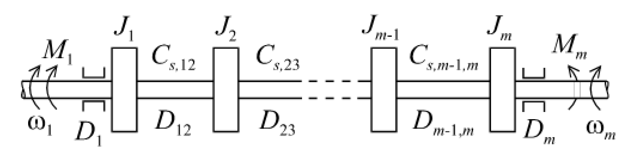
On the basis of the above-given assumptions, the kinematic structure of transmission shaft (Figure 1) transferred into m discrete elements was formulated [2], where J₁,…, J_m, C_s,12,…, C_s,m−1,m, S_c,12,…, S_c,m−1,m, D₁₂,…, D_m−1,m are the moments of inertia, coefficients of torsional stiffness, coefficients of torsional susceptibility (S_c = 1/C_s) and coefficients of viscous friction inside the respective elements of divided transmission shaft; D₁, D_m are the coefficients of friction defined for bearings.

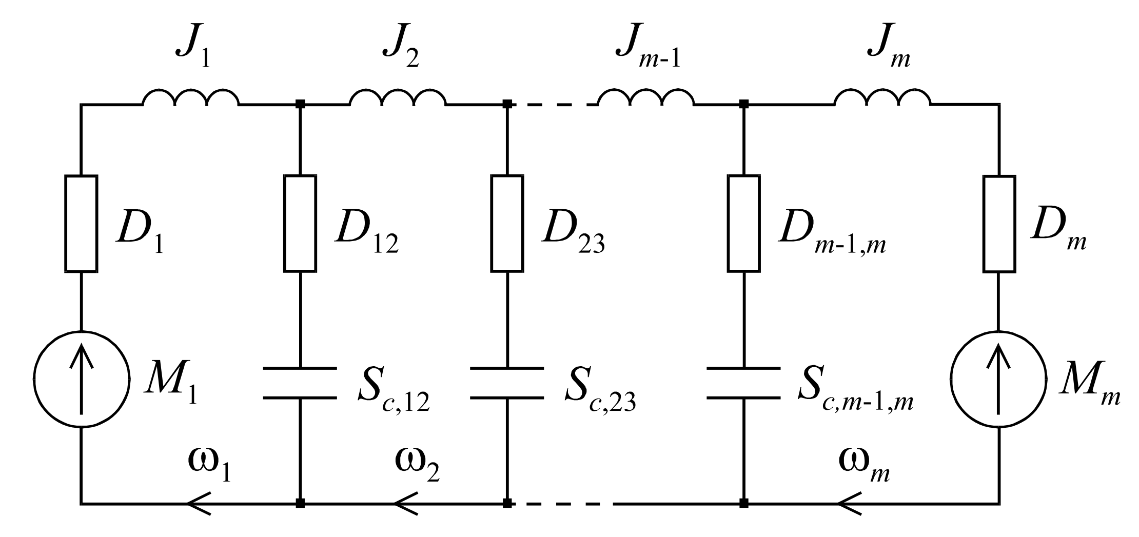
In accordance with the electromechanical energy conversion theory, the generalised coordinates are forces or torques in mechanical systems and voltages in electrical circuits, whereas the generalised velocities are the velocities or angular velocities in mechanical systems and currents in electrical systems. As a consequence, the parameters of transmission shaft are equivalent to those of the transmission line, i.e., the moment of inertia is equivalent to inductance, the torsional susceptibility is equivalent to capacitance, the coefficient of friction, if any, on the shaft surface is equivalent to the resistance and the coefficient of the viscous friction inside the shaft is equivalent to the inverse of the conductance. Adopting the abovementioned analogies and considering the specificity of transmission shaft, the equivalent circuits for the transmission shaft (Figure 2) has been created.

On the basis of the above given equivalent circuit the m equations of moments and torques as well as m−1 equations of angular velocities, corresponding with the Kirchhoff’s circuit laws typically applied in order to analyse electrical circuits, may be written for the mechanical coupling concerned [2]:

$$M_1-D_1{\mathsf{\omega }}_1-\frac{d}{dt}\left(J_1{\mathsf{\omega }}_1\right)-D_{12}\left({\mathsf{\omega }}_1-{\mathsf{\omega }}_2\right)-M_{c,12}=0,$$

(1)

$$\begin{gathered} M_{c,k-1,k}+D_{k-1,k}\left({\mathsf{\omega }}_{k-1}-{\mathsf{\omega }}_k\right)-D_{k,k+1}\left({\mathsf{\omega }}_k-{\mathsf{\omega }}_{k+1}\right)-\frac{d}{dt}\left(J_k{\mathsf{\omega }}_k\right)-M_{c,k,k+1}=0 \\ \mathrm{for} k=2,\dots ,m-1, \end{gathered}$$

(2)

$$M_{c,m-1,m}+D_{m-1,m}\left({\mathsf{\omega }}_{m-1}-{\mathsf{\omega }}_m\right)-\frac{d}{dt}\left(J_m{\mathsf{\omega }}_m\right)-D_m{\mathsf{\omega }}_m-M_m=0,$$

(3)

$${\mathsf{\omega }}_k-{\mathsf{\omega }}_{k+1}=\frac{d}{dt}\left(S_{c,k,k+1}{M}_{c,k,k+1}\right) \mathrm{for} k=1,\dots ,m-1.$$

(4)

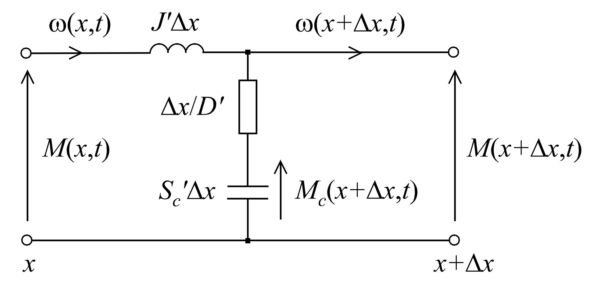
On the basis of the equivalent circuit (Figure 2) it can be concluded that the transmission shaft may be analysed in a similar way as the electric transmission line [2]. In order to formulate the distributed parameter model of transmission shaft, the following equivalent circuit of a shaft section, represented by the two-port system, can be used (Figure 3). The adopted length of the shaft section is Δx. It is assumed that the section Δx is short enough to use, in respect of this section, the dependencies adequate for the mathematical description of the lumped parameters model.

The equivalent circuit of transmission shaft section (Figure 3) is similar to that of the transmission line section [19]. There is a formal analogy between the lossless transmission shaft and the lossless transmission line.

Balancing moments of torsion around the closed-loop and angular velocities at the point leads to the following dependencies [2]:

$$M\left(x,t\right)=J^{\prime }∆x\frac{\partial \mathsf{\omega }\left(x,t\right)}{\partial t}+M\left(x+∆x,t\right),$$

(5)

$$\mathsf{\omega }\left(x,t\right)=S_c^{\prime }∆x\frac{\partial M_c\left(x+∆x,t\right)}{\partial t}+\mathsf{\omega }\left(x+∆x,t\right),$$

(6)

$$M\left(x+∆x,t\right)=D^{\prime }{S}_c^{\prime }\frac{\partial M_c\left(x+∆x,t\right)}{\partial t}+M_c\left(x+∆x,t\right),$$

(7)

where $J^{\prime }$, $D^{\prime }$, $S_c^{\prime }$ are specific (per unit of length) parameters of the shaft, i.e., specific moment of inertia, specific coefficient of friction and specific coefficient of torsional susceptibility, respectively, $S_c^{\prime }=\mathsf{\rho }/G{J}^{\prime }$, ρ is the mass density in kg/m³ and G is the shear module in GPa. Transforming Equations (5), (6) and (7) as well as assuming Δx → 0 the following equations can be obtained:

$$-\frac{\partial M\left(x,t\right)}{\partial x}=J^{\prime }\frac{\partial \mathsf{\omega }\left(x,t\right)}{\partial t},$$

(8)

$$-\frac{\partial \mathsf{\omega }\left(x,t\right)}{\partial x}=S_c^{\prime }\frac{\partial M_c\left(x,t\right)}{\partial t},$$

(9)

$$M_c\left(x,t\right)=M\left(x,t\right)+D^{\prime }\frac{\partial \mathsf{\omega }\left(x,t\right)}{\partial x}.$$

(10)

The further equations result from Equation (8) as well as Equations (9), (10) and (11):

$$-\frac{1}{J^{\prime }}\frac{{\partial }^{2}M\left(x,t\right)}{\partial x^2}=\frac{{\partial }^2\mathsf{\omega }\left(x,t\right)}{\partial x\partial t},$$

(11)

$$-\frac{\partial \mathsf{\omega }\left(x,t\right)}{\partial x}=S_c^{\prime }\frac{\partial M\left(x,t\right)}{\partial t}-\frac{S_c^{\prime }{D}^{\prime }}{J^{\prime }}\frac{{\partial }^{2}M\left(x,t\right)}{\partial x^2}.$$

(12)

A lossless transmission shaft may also be considered, if $D^{\prime }=0$:

$$-\frac{\partial M\left(x,t\right)}{\partial x}=J^{\prime }\frac{\partial \mathsf{\omega }\left(x,t\right)}{\partial t},\hspace{1em}\hspace{1em}-\frac{\partial \mathsf{\omega }\left(x,t\right)}{\partial x}=S_c^{\prime }\frac{\partial M\left(x,t\right)}{\partial t}.$$

(13)

If the shaft parameters do not change along the axis, Equation (13) may be decoupled in respect of moment of torsion and angular velocity:

$$-\frac{{\partial }^{2}M}{\partial x^2}=J^{\prime }{S}_c^{\prime }\frac{{\partial }^{2}M}{\partial t^2},\hspace{1em}\hspace{1em}-\frac{{\partial }^2\mathsf{\omega }}{\partial x^2}=J^{\prime }{S}_c^{\prime }\frac{{\partial }^2\mathsf{\omega }}{\partial t^2},$$

(14)

$$-\frac{{\partial }^{2}M}{\partial x^2}=\frac{1}{v^2}\frac{{\partial }^{2}M}{\partial t^2},\hspace{1em}\hspace{1em}-\frac{{\partial }^2\mathsf{\omega }}{\partial x^2}=\frac{1}{v^2}\frac{{\partial }^2\mathsf{\omega }}{\partial t^2},\hspace{1em}v=\frac{1}{\sqrt{J^{\prime }{S}_c^{\prime }}}=\sqrt{\frac{G}{\mathsf{\rho }}},$$

(15)

where v is phase velocity in m/s. The general solution of the equations of type (15) was given by d’Alembert [19]:

$$M\left(x,t\right)=\frac{1}{2}\left[M_1\left(t+\frac{x}{v}\right)+M_1\left(t-\frac{x}{v}\right)\right]+\frac{v}{2}{{\displaystyle \int }}_{t-\frac{x}{v}}^{t+\frac{x}{v}}\frac{\partial M\left(0,\mathsf{\tau }\right)}{\partial x}d\mathsf{\tau },$$

(16)

with the boundary conditions:

$$M_1\left(t\right)={\left.M\left(x,t\right)\right|}_{x=0},\hspace{1em}\hspace{1em}\frac{\partial M\left(0,t\right)}{\partial x}={\left.\frac{\partial M\left(x,t\right)}{\partial x}\right|}_{x=0}.$$

(17)

On the basis of the first Equation (13) and the Equation (16) the following Equations (18), (19) and (20) may be written:

$$\frac{\partial M\left(0,t\right)}{\partial x}=-J^{\prime }\frac{\partial \mathsf{\omega }\left(0,t\right)}{\partial t}=-J^{\prime }\frac{\partial {\mathsf{\omega }}_1\left(t\right)}{\partial t},$$

(18)

$$\frac{v}{2}{{\displaystyle \int }}_{t-\frac{x}{v}}^{t+\frac{x}{v}}\frac{\partial M\left(0,\mathsf{\tau }\right)}{\partial x}d\mathsf{\tau }=-\frac{1}{2}\sqrt{\frac{J^{\prime }}{S_c^{\prime }}}{{\displaystyle \int }}_{t-\frac{x}{v}}^{t+\frac{x}{v}}d{\mathsf{\omega }}_1\left(\mathsf{\tau }\right)=-\frac{z_v}{2}\left[{\mathsf{\omega }}_1\left(t+\frac{x}{v}\right)-{\mathsf{\omega }}_1\left(t-\frac{x}{v}\right)\right],$$

(19)

$$M\left(x,t\right)=\frac{1}{2}\left[M_1\left(t+\frac{x}{v}\right)+M_1\left(t-\frac{x}{v}\right)\right]-\frac{z_v}{2}\left[{\mathsf{\omega }}_1\left(t+\frac{x}{v}\right)-{\mathsf{\omega }}_1\left(t-\frac{x}{v}\right)\right],$$

(20)

where z_v is wave impedance, $z_v=\sqrt{J^{\prime }/S_c^{\prime }}=v{J}^{\prime }$. The analogous formula for calculation of angular velocity may also be written as follows:

$$\mathsf{\omega }\left(x,t\right)=\frac{1}{2}\left[{\mathsf{\omega }}_1\left(t+\frac{x}{v}\right)+{\mathsf{\omega }}_1\left(t-\frac{x}{v}\right)\right]-\frac{1}{2z_v}\left[M_1\left(t+\frac{x}{v}\right)-M_1\left(t-\frac{x}{v}\right)\right].$$

(21)

On the basis of the Equations (20) and (21) the moments of torsion at the shaft beginning (input) and the shaft end (output) may be expressed as follows:

$$M_1\left(t\right)=z_v{\mathsf{\omega }}_1\left(t\right)-z_v{\mathsf{\omega }}_m\left(t-\frac{l}{v}\right)+M_m\left(t-\frac{l}{v}\right),$$

(22)

$$M_m\left(t\right)=-z_v{\mathsf{\omega }}_m\left(t\right)+z_v{\mathsf{\omega }}_1\left(t-\frac{l}{v}\right)+M_1\left(t-\frac{l}{v}\right),$$

(23)

where l is the shaft length. The abovementioned moments of torsion may also be expressed in the discrete form:

$$M_1\left(j\right)=z_v{\mathsf{\omega }}_1\left(j\right)-z_v{\mathsf{\omega }}_m\left(j-n\right)+M_m\left(j-n\right),$$

(24)

$$M_m\left(j\right)=-z_v{\mathsf{\omega }}_m\left(j\right)+z_v{\mathsf{\omega }}_1\left(j-n\right)+M_1\left(j-n\right),$$

(25)

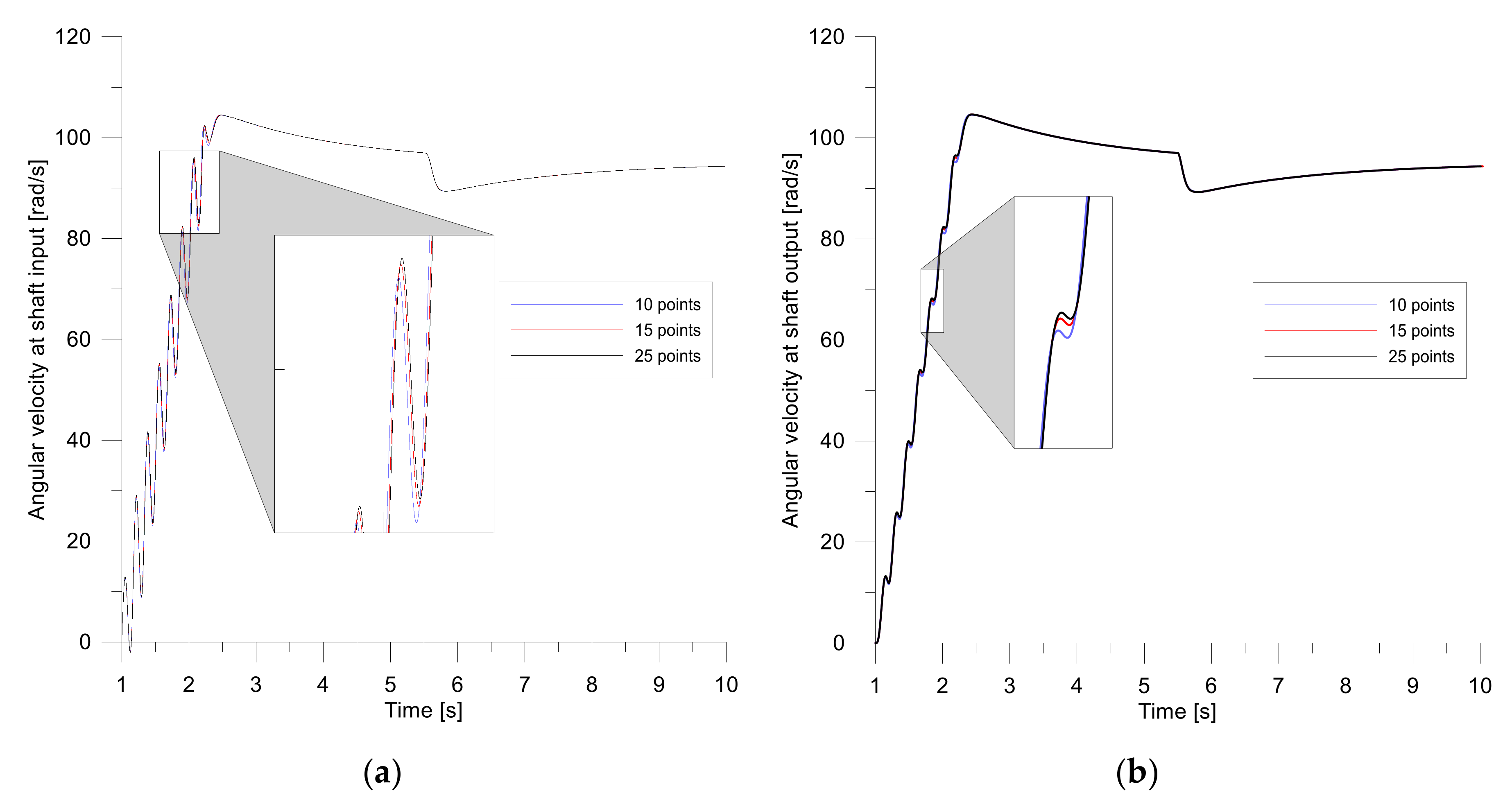
with the initial conditions M₁(0), M_m(0), ω₁(0) and ω_m(0), where: n is the number of numerical calculation points, $n=l/vh$, h is the width of the step size between the points, j = 0,1,…. The number n is also a discrete-time of moving the mechanical wave from one end of the shaft to the other. The continuous-time of moving the wave along the shaft axis, corresponding with number n, is given in the Equations (22) and (23) as $l/v$. The optimum number of numerical calculation points is the number, the increase of which does not cause significant differences in simulation results, whereas the decrease of this number causes significant differences in simulation results. The terms from the previous steps ω(j–n) and M(j–n) in the Equations (24) and (25) may be determined using shift registers. For j ≤ n:

$$M_1\left(j\right)=z_v{\mathsf{\omega }}_1\left(j\right),\hspace{1em}{M}_m\left(j\right)=-z_v{\mathsf{\omega }}_m\left(j\right).$$

(26)

The angular velocities at the beginning (input) and the end (output) of the transmission shaft may be calculated on the basis of the equations of motion for the rotors of both an electric motor and working machine:

$$J_e\frac{d{\mathsf{\omega }}_1\left(t\right)}{dt}=M_e\left(t\right)-D_1{\mathsf{\omega }}_1\left(t\right)-M_1\left(t\right),$$

(27)

$$J_L\frac{d{\mathsf{\omega }}_m\left(t\right)}{dt}=M_m\left(t\right)-D_m{\mathsf{\omega }}_m\left(t\right)-M_L\left(t\right),$$

(28)

where M_e(t) and M_L(t) are motor output torque and a load torque of working machine, J_e and J_L are moments of rotor inertia for motor and working machine, respectively, D₁ and D_m are coefficients of friction defined for bearings.

The model with two lumped damping parameters D_1m and D_m1 may be adopted in order to represent the viscous friction inside the shaft. Then, the Equations (27) and (28) take the following form:

$$J_e\frac{d{\mathsf{\omega }}_1\left(t\right)}{dt}=M_e\left(t\right)-D_1{\mathsf{\omega }}_1\left(t\right)-D_{1m}\left({\mathsf{\omega }}_1\left(t\right)-{\mathsf{\omega }}_m\left(t\right)\right)-M_1\left(t\right),$$

(29)

$$J_L\frac{d{\mathsf{\omega }}_m\left(t\right)}{dt}=M_m\left(t\right)-D_m{\mathsf{\omega }}_m\left(t\right)-D_{m1}\left({\mathsf{\omega }}_m\left(t\right)-{\mathsf{\omega }}_1\left(t\right)\right)-M_L\left(t\right).$$

(30)

Such an extension of the model allows for maintaining the advantageous features resulting from the simplicity of numerical calculations.

3. Simulations and Experimental Results

Research Implementation Methods

To verify the proposed solution of the long driveshaft modelling algorithm by the use of an electric transmission line, simulation and experimental research were performed. In the first step, the algorithm computer program in C++ programming language was written by the research team. Open and free software was used to write the simulation program. The development of a simulation program independently enables the optimization of the algorithm code that is to be implemented in the future in an inverter with a digital signal processor.

The simulation contains the brushless dc motor (BLDC) model with a full control system, long driveshaft model according to Equations (24) and (25) and a direct current generator model. In the simulation, the parameters of 4 kW BLDC motor and steel transmission shaft of length 0.66 m and diameter 0.008 m, according to the real laboratory setup elements, were taken. Other parameters of the simulation model and reference units are shown in

Table 1. Model parameters.

Parameter	Symbol	Value
Length of shaft	l	0.66 m
Diameter of shaft	d	0.008 m
Specific moment of inertia	$J^{\prime }$	3,18·10−6 kg·m2/m
Specific coefficient of friction	$D^{\prime }$	7.3·10−3 Nm2s
Specific coefficient of torsional susceptibility	$S_c^{\prime }$	32·10−3 1/Nm2
Wave impedance	zv	0.01 Nms
Mass density	ρ	7900 kg/m3
Shear module	G	77.5 GPa
Phase velocity	v	3132 m/s
Motor output torque	Me	N·m
Load torque	ML	N·m
Moment of rotor inertia for motor	Je	0.025 kg·m2
Moment of inertia for load	JL	0.11 kg·m2
Moment of inertia for additional elements	Ja	0.079 kg·m2
Coefficients of friction for bearings	D1; Dm	1.6·10−3 Nms
Lumped damping parameters representing viscous friction inside the shaft	D1m, Dm1	0.022 Nms

.

In order to determine the optimum number of numerical calculation points, the numerical simulations of the transmission shaft behaviour were carried out, in which various numbers of numerical calculation points n were taken into account, respectively, 10, 15, 20 and 25 points. Figure 4 shows angular velocities for beginning (input) and end (output) of the transmission shaft for different calculations variants. The end of the transmission shaft was loaded by a rotating mass J_L = 0.11 kg·m² and a mechanical torque of rated value.

Figure 5; Figure 6 show respective the differences in angular velocity and angle of twist for the transmission shaft for different calculations variants.

If a lower number of numerical calculation points is chosen (10 and 15) then the effect similar to the shortening of the shaft occurs (slightly less amplitude of oscillation and slightly less natural frequency as well as the decrease of steady angle of twist after 8 s from starting the system at the time t = 1 s).

For 20 and 25 points, the differences in amplitude of oscillation, natural frequency and steady angle of twist are not significant. It can be read from the graphs. For example, the difference in amplitude of oscillation and difference in steady angle of twist for 10 and 25 points, respectively, is in a range of 1 degree, which is around 5% in respect to the steady angle of twist, whereas for 20 and 25 points, respectively, this difference is a fraction of a percentage. The differences can disappear for an infinite number of points; therefore, a balance between the accuracy of numerical calculations and the speed of numerical calculations should be found.

In the next step, the simulation results were verified by the experiment. Experimental investigations were made using a test stand including a BLDC motor coupled with a DC generator by a steel long driveshaft. The parameters of the shaft (length, diameter) in the experimental setup was designed in accordance with the power of experimental setup components. This setup allows for connecting the shafts of various diameters, which allow for a good representation of the parameters of real-world systems. The laboratory setup is shown in Figure 7. In addition, in the figure, a simplified diagram of an experimental stand layout corresponding to the actual configuration was presented. The test stand is fully configurable; therefore, it is possible to mount additional steel discs at the shaft on the DC generator side that allow to change the moment of inertia of the load. Two rotary incremental encoders with a resolution of 3600 pulse/rev installed on the transmission shaft ends, are used to measure angular displacement and angular velocities. Hall effects transducers were used to measure motor phase currents. The measuring signals from the transducers are sent to a laboratory computer equipped with two multifunctional I/O devices PCIe-6351 from National Instruments.

Laboratory Virtual Instrument Engineering Workbench (LabVIEW) was used for data collection, whereas a computer program to visualise the measurement datasets was created by the authors. The test stand is fully automated and allows testing of the driveshaft with different geometries and made of different materials.

All presented time waveforms correspond to starting the motor and the operation under rated load after 5.5 s. The characteristic time waveforms for angular velocities at shaft input and output, the difference in angular velocity, angle of twist and phase current of BLDC motor, are shown in Figure 8, Figure 9, Figure 10, Figure 11, Figure 12.

High similarity of both the experimental results confirms good accuracy of the proposed model.

4. Discussion

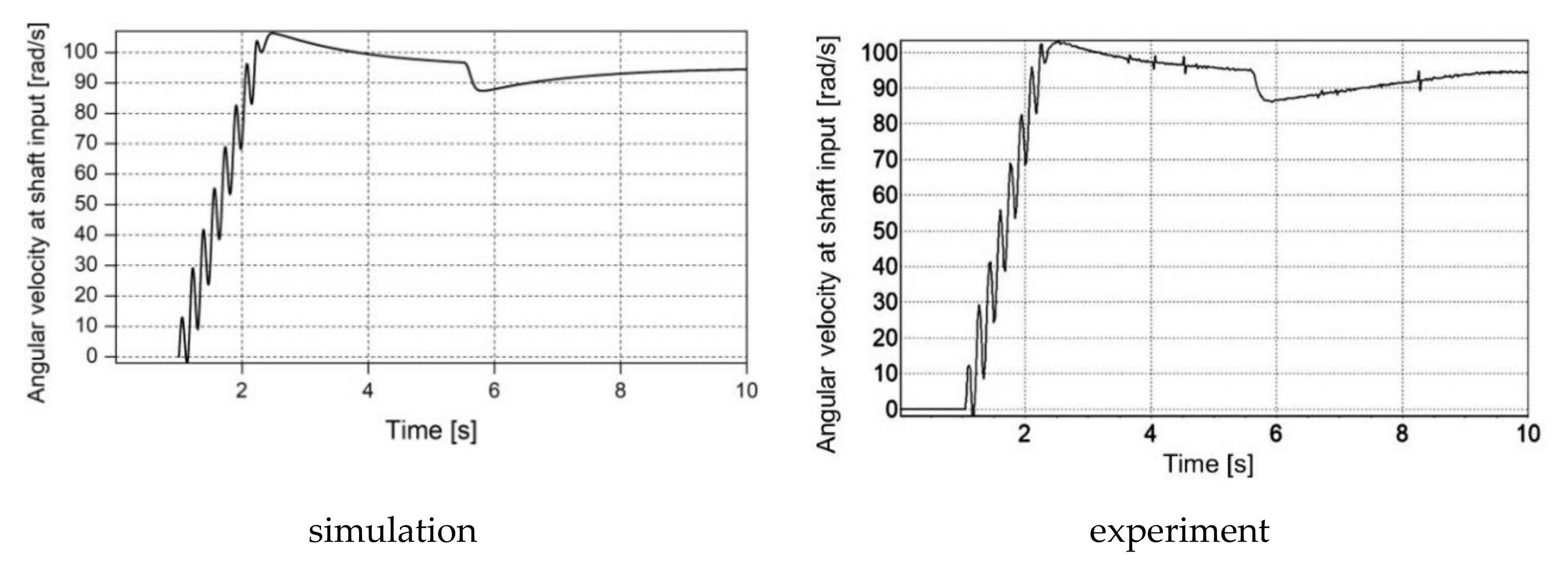
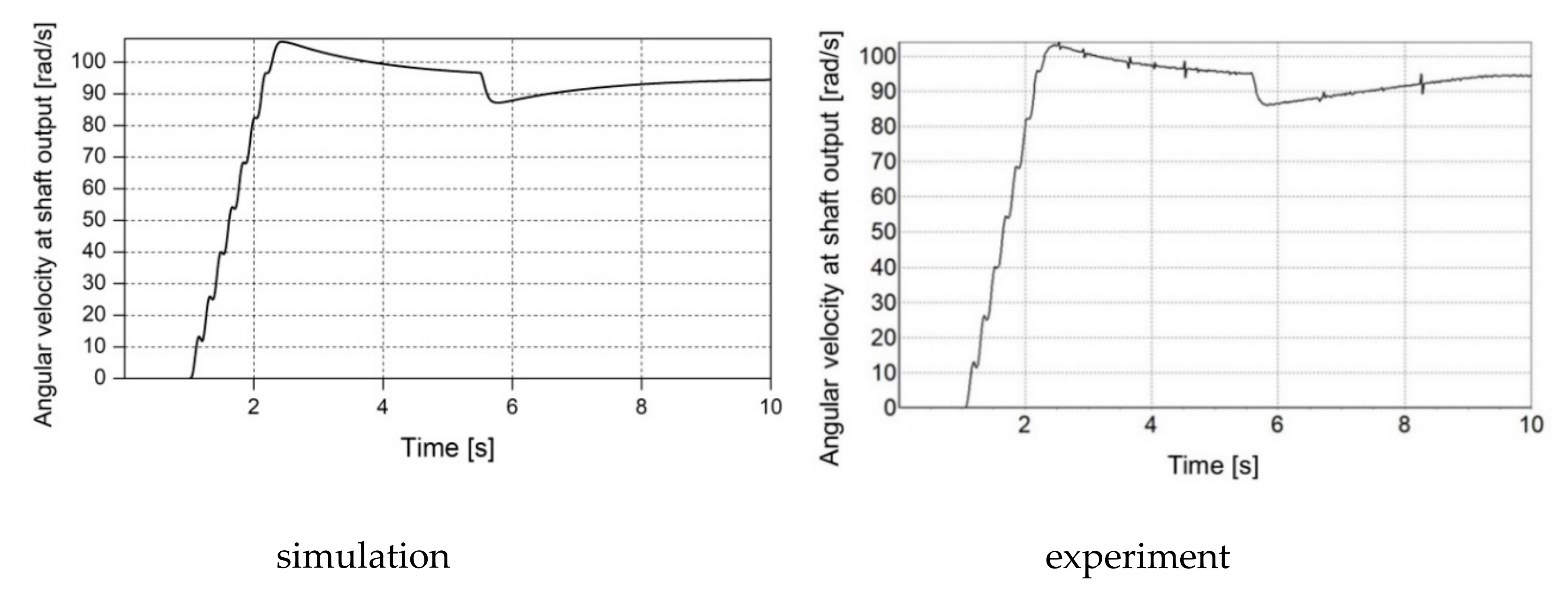
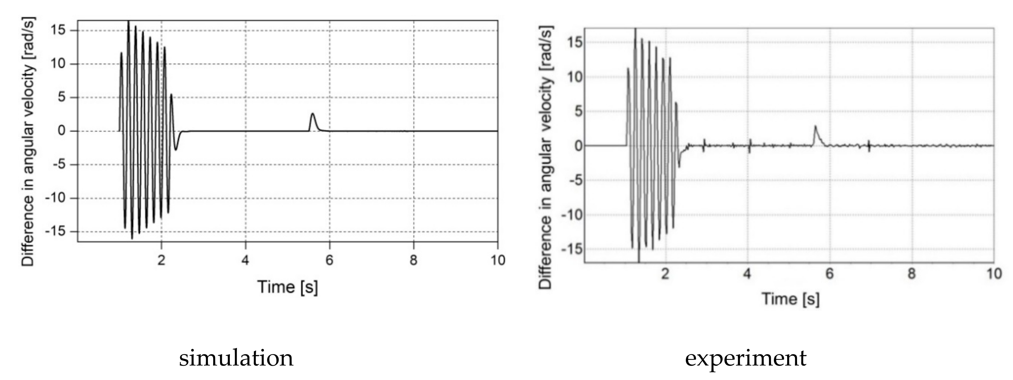
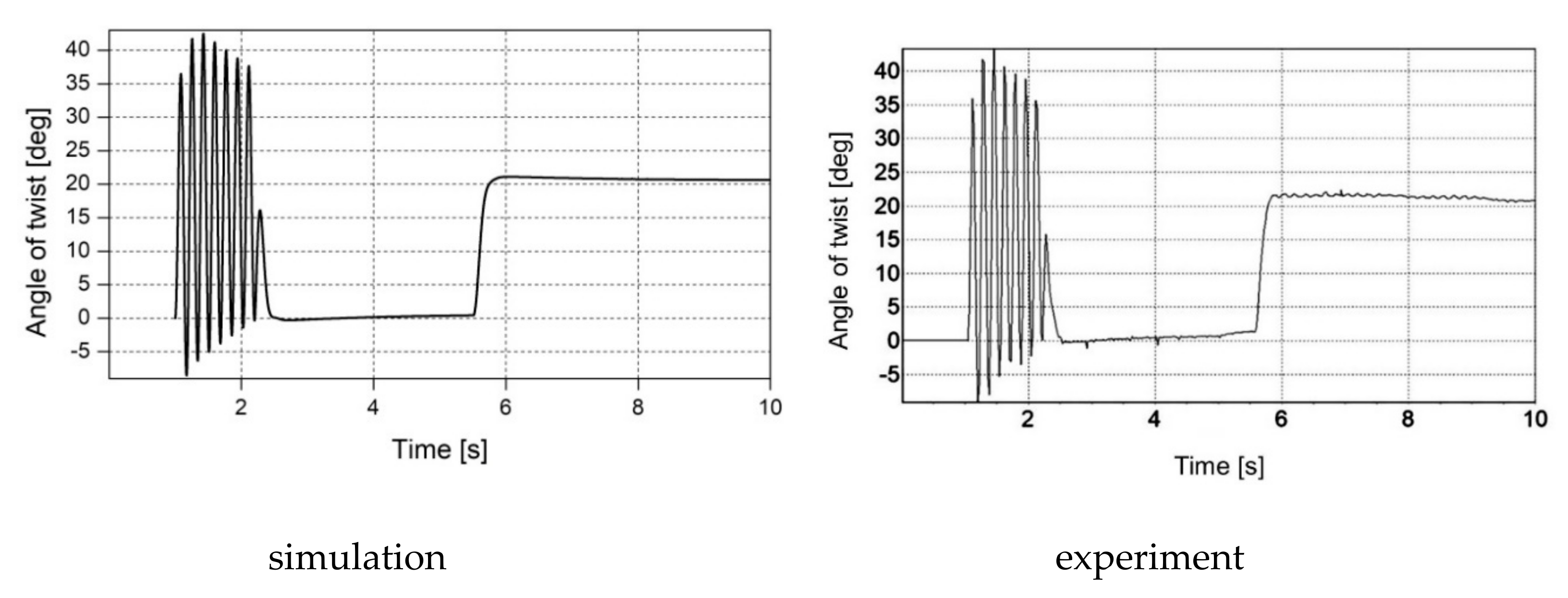
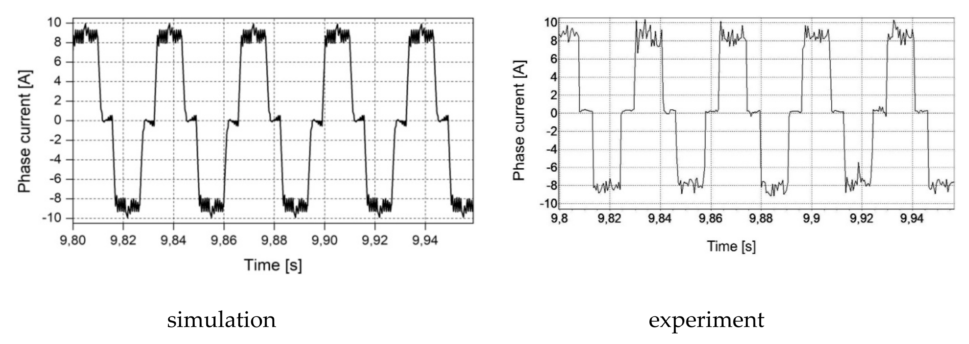
The results of the computer simulation and experimental tests presented in the paper deal with the modelling of the transmission shaft being a mechanical component of an electric drive. The high similarity of both experimental and simulation results confirms the high conformity of the proposed mathematical model, based on electrical and mechanical similarities with the physical object. This conformity is crucial from a practical point of view for design activities.

The telegrapher’s equations and their d’Alembert solution are proposed in the article for the mathematical description of the transmission shaft. If the boundary conditions for the two points at the ends of the shaft are adopted, the solution is determined only for these points, without the need to track the processes within the shaft. If the shaft is part of a complex system, including an electric motor, power converter, mechanical coupling and working machine, then only the variables at the shaft ends can be taken into account, without the need to estimate the phenomena for any other value of shaft axis coordinate x. This assumption leads to the very simple equations of the discrete model of the lossless transmission shaft. This approach is known as Bergeron diagram method. The solution of the abovementioned equations does not require numerical integration, which can cause a problem with the stability of the integration method and it is often carried out in more than one stage. As a consequence, a shorter time for carrying out the numerical calculations is required if the proposed model is used than in the case of the models based on differential equations. Thus, high accuracy of the proposed model goes hand in hand with its simplicity and, as a consequence, with a short time of numerical calculations in contrast to the modelling based on numerical integration of differential equations or analytical solution of partial differential equations. For example, in the case of the multi-mass model of the transmission shaft divided into m discrete elements, 2m − 1 ordinary differential equations have to be integrated numerically k times for each step, where k is the order of numerical integration method. The use of the proposed model, based on the d’Alembert solution for telegrapher’s equations, requires for each step the single numerical calculation of 4n − 2 discrete equations of type X [j + 1] = X [j] and 2 discrete equations given in the article as (24) and (25), where n depends on the shaft length, phase velocity and width of the step size in accordance with dependency given in the article. In order to ensure high accuracy of numerical integration of ordinary differential equations, which is comparable with the accuracy of numerical calculation of the discrete equations included in the proposed model, the width of the step size for the numerical integration should be tens of times shorter than for the numerical calculation of the abovementioned discrete equations. This means that using the proposed model leads to less numerical calculations in the same unit time than for the models based on differential equations.

5. Conclusions

Long elastic elements, especially transmission shafts, may be described mathematically by multi-mass lumped parameter models based on ordinary differential equations or distributed parameter models based on partial differential equations, which may be solved analytically. However, the analytical solution is both tedious and time-consuming. Thus, partial differential equations are usually transformed into ordinary differential equations by using finite differences. In both the abovementioned cases, the ordinary differential equations are usually integrated numerically.

In the paper, the kinematic structure of the transmission shaft between the driving motor and the working mechanism is studied. The analysis is based on electrical and mechanical similarities. The equations of moments and angular velocities, analogous to the Kirchhoff’s law-based equations typically applied in the mathematical analysis of branched electrical circuits, are defined. Modelling of transmission shaft based on a formal analogy between the transmission shaft and the electric transmission line is also proposed. The high conformity of the proposed mathematical model with the physical object has been confirmed by the comparison of the results of computer simulation and experimental tests.

The advantage of the proposed model is its simplicity, due to the fact that the model bases on discrete equations, which do not require numerical integration in contrast to the models based on differential equations. The presented approach to modelling of the entire electromechanical system can be easily developed towards the system containing more than one elastic coupling, electric motor or working machine.

The proposed mathematical model may be used to analyse the impact of control and load on an electromechanical system as well as the failure states associated with or close to the resonance phenomenon. Simulation results may be used to design electric drives as well as to optimise electromechanical systems during operation.

The proposed transmission shaft model based on discrete equations is an open-loop model, but nothing precludes its use in a closed-loop control system in an advanced electric drive. This will be the subject of further research work of the authors team.