Article

Indirect Methods for Validating Shallow Geothermal Potential Using Advanced Laboratory Measurements from a Regional to Local Scale—A Case Study from Poland

1
Faculty of Geology, Geophysics and Environmental Protection, AGH University of Science and Technology, Mickiewicza 30 Av., 30-059 Kraków, Poland
2
Oil and Gas Institute—National Research Institute, Lubicz Str. 25A, 31-503 Kraków, Poland
*
Authors to whom correspondence should be addressed.
Energies 2020, 13(20), 5515; https://doi.org/10.3390/en13205515
Submission received: 4 August 2020 / Revised: 20 September 2020 / Accepted: 19 October 2020 / Published: 21 October 2020
(This article belongs to the Special Issue Geothermal Resources)

Abstract

:
This paper presents a broad overview of laboratory methods for measuring thermal properties and petrophysical parameters of carbonate rocks, and analytical methods for interpreting the obtained data. The investigation was conducted on carbonate rock samples from the Kraków region of Poland in the context of shallow geothermal potential assessment. The measurement techniques used included standard macroscopic examinations; petrophysical investigations (porosity, density); analysis of mineral composition thermal conductivity (TC) and specific heat measurements; and advanced investigations with the use of computed tomography (CT). Various mathematical models, such as layer model, geometric mean, and spherical and non-spherical inclusion models, were applied to calculate thermal conductivity based on mineralogy and porosity. The aim of this paper was to indicate the optimal set of laboratory measurements of carbonate rock samples ensuring sufficient characterization of petrophysical and thermal rock properties. This concerns both the parameters directly characterizing the geothermal potential (thermal conductivity) and other petrophysical parameters, e.g., porosity and mineral composition. Determining the quantitative relationship between these parameters can be of key importance in the case of a shortage of archival thermal conductivity data, which, unlike other petrophysical measurements, are not commonly collected. The results clearly show that the best correlations between calculated and measured TC values exist for the subgroup of samples of porosity higher than 4%. TC evaluation based on porosity and mineral composition correlation models gives satisfactory results compared with direct TC measurements. The methods and results can be used to update the existing 3D parametric models and geothermal potential maps, and for the preliminary assessment of geothermal potential in the surrounding area.

1. Introduction

Energy policies and climate protection are, in addition to safety issues, some of the most important global challenges at the present time. One of the main elements of climate protection is energy transformation, particularly in the fast-developing countries of Asia (China, India, etc.) and East Europe, where the share of fossil fuel, comprised mainly of coal and natural gas, remains dominant in particular industries and heating.
According to the latest statistical data, in 2017 the global share of fossil fuels in the total consumption of final energy was calculated to be 79.7% [1] and the share of renewable sources of energy for heating and cooling in Europe (EU-28) was estimated to be 19.5%. In Poland, renewable sources accounted for only 14.5% of total energy consumption [2]. A considerable portion of the heat and cooling production balance in EU-28 relates to heat pump technology using aerothermal and geothermal energies, which in 2017 were responsible for 5% and 3% of the total energy production from renewable energy sources, respectively [2].
The share of heat pump technology in Poland in the production of energy from renewable sources by carriers is negligible, accounting for 0.6% for ambient heat pumps, and 0.2% when considering overall geothermal heat sources [2]. Despite the current low share in total heat production, Poland is recognized as the fourth largest heat pump market in Europe in terms of annual sales [3]. This situation has resulted not only from raising awareness of environmental issues but is also due to the adopted declarations on the reductions of emissions. Globally, Poland is ranked the 18th largest emitter of carbon dioxide and 3rd amongst EU members [4].
Energy transformation in Europe and Poland requires intensive action to be undertaken until 2030, because the consumption of primary energy for heating and cooling remains the greatest share of the energy sector. In the response to EU documents, national obligations concerning energy and climate were summarized in “National plan for energy and climate for years 2021–2030. Assumptions and aims as well as action policy” [5], which, on 30 December 2019, were passed by the European Commission.
These national commitments were also reflected in regional policies; for example, in Małopolska Province, from 2026 the combustion of solid fuels will be permitted only in so-called “Class (V) heating devices” [5] or in those fulfilling the ecodesign directive. From 1 October 2017 production of solid fuels boilers below class (V) were prohibited in Poland; similarly, since 1 July 2018 the sale of these boilers was prohibited [6].
The use of heat pump technology can thus play a vital role in measures to reduce smog, particularly in Kraków and surrounding areas, where alternative effective renewable energy sources have yet to be found. Air pollution, caused mainly by the general use of natural solid fuels for heating, remains one of the most important development problems in Poland. In this regard, in 2016, the Małopolska Provincial Assembly passed an anti-smog resolution introducing a total ban on the combustion of coal and other solid fuels within the city, which came into force on 1 September 2019 [7]. Despite considerable investments by the town carried out by the Municipal District Heating Enterprise (MPEC S.A.), due to numerous technical and/or economic factors ~35% of Kraków residents have yet to be connected to the district heating network. One means to diversify heat sources and reduce emissions in and around Kraków, as indicated by the Kraków Municipality Office, is by using heat pumps.
Estimates made within the GeoPLASMA-CE [8] project indicate that in the region of Kraków a considerable shallow geothermal potential exists, both in rocks and in ground water. The assessed inventory showed that about 200 small and 24 bigger geothermal heat pump installations with a total capacity of approximately 5 MWt were operational in Kraków at the end of 2018 [9]. These estimations do not include heat pumps with a horizontal heat exchanger and air heat pumps. The total length of borehole heat exchangers (BHEs) of these installations was estimated to be about 92 km [9].
An optimistic scenario of shallow geothermal heat development, e.g., maintaining a 5% yearly increase in heat pump sales in the Polish market [10], implies that thermal power installed in Kraków in 2050 can be forecast to be about 22 MWt [8]. Considering the town’s heat demand in 2018 was estimated to be about 1807 MWt [11], in 2050 geothermal heat pumps could account for about 1.2% of this demand (the present share of heat pump technology in the total balance of heat production in Kraków is less than 0.3% [8]). The development of heat pump technology can assist in the improvement of air conditions and increase the total share of renewable energy sources in Poland’s final energy consumption.
To meet the environmental requirements resulting from the adopted declarations, which introduced a total ban on the combustion of solid fuels in Kraków, the AGH University of Science and Technology, and the Municipal District Heating Enterprise S.A. (heat provider), signed an agreement on 7 May 2019 to cooperate in the use of renewable energy sources in distributed systems. The main goal of the cooperation is to analyze the possibilities and scale of using heat pump technology, including ground source heat pumps (GSHPs) in Kraków, as a supplement to the company’s district heating system. This applies to locations beyond the reach of the heating network, as mentioned previously.
Knowledge of the potential of shallow geothermal energy, including thermal conductivity distribution, is an important factor in the sustainable development of the heat pump market and a tool to assist in the reduction of low emissions in Kraków.
Thermal conductivity of the geological profile is a crucial parameter for designing borehole heat exchangers (BHEs). Thermal conductivity can play a significant role in cases in which no thermal response test (TRT) is available, which is common for small installations, i.e., those not exceeding 30–50 kW. In simple terms, thermal conductivity controls the size of the ground volume, which effectively transfers heat towards pipes in BHEs. The higher the thermal conductivity, the bigger the ground volume involved and the greater the available energy. In terms of vertical scale, higher thermal conductivity provides the opportunity to obtain higher ground temperatures at a shallow depth because the ground conducts the Earth’s heat more efficiently. Higher temperatures provide higher heat pump efficiency and greater energy available from the ground in the case of unbalanced exploitation.
The knowledge of thermal conductivity of the geological profile allows optimal design of the BHE. In particular, design of the total depth of wells what can significantly reduce the risk of under- or overestimating the BHE heat output and ensure long-term effective operation of the entire heat pump system. Thermal conductivity values are characterized by a considerable degree of diversity among different lithologies and particular lithological types. As a result, the assessment of rocks’ thermal properties for shallow geothermal energy should not only be based on literature data but, if possible, on thermal response tests or laboratory measurements performed on samples of particular rock formations in the investigated region.
Thermal conductivity of rock can be also calculated using mathematical models based on the rock’s components. This issue has been addressed by many authors [12,13,14,15,16,17,18,19,20,21,22]. A comprehensive overview of different models was presented by Schön [12]. Zimmerman [20] introduced a theoretical model for prediction of the thermal conductivity of fluid-saturated rocks, in which the rock is composed of connected mineral phases permeated with non-intersecting oblate spheroidal pores. Converting matrix thermal conductivity into thermal conductivity of saturated rock was described by Fuchs [16]. Pimienta et al. [15] compared measured thermal conductivity, thermal diffusivity, and P-wave velocity with model predictions. Comparing measured and modeled data, they distinguished three groups of sandstone samples varying in quartz content and porosity. Correlations of calculated thermal conductivity with P-wave velocity depending on the rock type were also described by Gegenhuber [13]. Middleton [18] presented a method of determining matrix thermal conductivity from dry drill cuttings and tested the obtained empirical formula by comparing it with modelled thermal conductivity values. Goutorbe et al. [14] compared the values predicted from geophysical well logs with the use of neural networks and mathematical models. In other works [17,19], the lithological profiles and porosity obtained from geophysical logs were used as the input data for calculating thermal conductivity on the base of mathematical models. The authors used the models to calculate thermal conductivity of the Carpathian sandstones [21,22].

2. Objectives

The aim of this paper was to indicate the optimal set of laboratory measurements of carbonate rock samples that ensure sufficient characterization of petrophysical and thermal rock properties. This concerns both the parameters directly characterizing the geothermal potential (thermal conductivity) and other petrophysical parameters (porosity and mineral composition).
Here, a wide range of investigations and laboratory measurements were conducted, ranging from standard mineralogical analyses and petrophysical measurements of density and porosity, and thermal conductivity and heat capacity, to advanced methods using computed tomography techniques. The obtained data were applied to calculate thermal conductivity with the use of different mathematical models. Determining the thermal conductivity based on other parameters can be of key importance in the case of a shortage of archival thermal conductivity analyses, which, unlike other petrophysical measurements, are not commonly performed.
The conducted investigations and measurements will both extend the scant base of the petrophysical and thermal parameters of the rocks of the Kraków region, and broaden the knowledge on applicable measurement methods and eventual limitations in their application. A second aim was to indicate the appropriate methods for performing laboratory measurements and data analysis that can be applied to carbonate rocks in other locations.

3. Theoretical Background

Thermal conductivity depends on petrophysical parameters such as mineral composition, porosity, grain size, degree of cementation, size and shape of pores, the presence of fractures and cavities, and pressure and temperature. These parameters should be considered in the analysis of the obtained laboratory thermal conductivity values. The most important parameters, with a brief description of their possible impact on thermal conductivity, are listed below.
Mineral composition and lithology—the thermal conductivity of a rock increases with higher contents of minerals with high thermal conductivity. Particularly important is the influence of quartz, which is abundant in many rock types and is characterized by a high thermal conductivity value (Table 1). Clay minerals, mainly those of the mica group (Table 1), have low thermal conductivity values. Thus, sandstones, particularly quartz sandstones, display higher thermal conductivity values than mudstones and claystones. Values for carbonate rocks are close to average, and are higher in the case of dolomites than limestones (Figure 1). Felsic igneous rocks are characterized by higher thermal conductivity than the alkaline rocks (Figure 1).
Porosity—the thermal conductivity coefficient value decreases with an increase in porosity because both the air and media saturating the pore space are characterized by a considerably lower thermal conductivity than the rock framework. The thermal conductivity of water is 0.61 W/m∙K; oil, 0.14 W/m∙K; and air, 0.026 W/m∙K [12,29].
Fractures and cavities—these can be of great significance in the case of igneous, metamorphic, and carbonate rocks. The thermal conductivity value is influenced by the number of fractures in addition to their geometry, and by the properties of the filling substances [12]. The presence of fractures is also connected with a higher vulnerability of rock to pressure changes. With an increase in pressure, the fractures close and the thermal conductivity values significantly increase [12].
Grain size—the thermal conductivity value increases with the size of the grain. This is due to the decreased contact between grains and, subsequently, lower resistance between grain contacts [30,31].
Rock structure—anisotropy influences the heat flow rate; thus, in the case of rocks with an orientated structure, the thermal conductivity value depends on the measurement direction [12,13,29,32]. The anisotropy of thermal conductivity is determined by the coefficient , which is defined as the ratio of the λ value measured parallel to rock structure (λǁ) to λ values measured perpendicularly (λ⏊). The highest values are characteristic of shales, schists, and gneisses, and the lowest for carbonate rocks [29,32].
Pressure—better heat flow in grain contacts, tightening fractures, and decreasing porosity caused by increasing pressure result in higher thermal conductivity [12]. Experiments conducted on mudstone and dolomite have shown that the thermal conductivity increases with an increase in pressure up to circa 80 MPa and then stabilizes [33].
Temperature—thermal conductivity depends on temperature. This relationship is connected to the structure of the material. With increasing temperature, the thermal conductivity of crystalline materials (such as minerals) decreases, and increases in the case of amorphous materials. For the majority of rocks, the thermal conductivity decreases as temperature increases [12].
To summarize, the thermal conductivity value of a rock is a function of both the content and the thermal conductivity of the rock’s minerals and media saturating the pore space. It also depends on the pore space structure. Thus, when assessing this parameter, different models can be applied based on a simplification of the rock’s internal geometry (structure), allowing for calculation of the rock thermal conductivity based on the properties of its components [12,13,14,15,16,17,18,19,20,21,22].
To determine thermal conductivity, various mathematical models have been applied, from simple layer models, to more sophisticated spherical and non-spherical inclusion models.

3.1. Layer Models

The layer models in which the heat flow is parallel or perpendicular to the boundary between components is assumed to determine the extreme values, i.e., limits within which the true thermal conductivity values are placed [12,17,20].
The thermal conductivity for the heat flow parallel to the boundary between components is defined by the arithmetic mean (λ_aryt), thus determining the upper limit of the investigated value [12,17,20]:
λ _ a r y t = ( 1 ϕ ) λ m + ϕ λ f
where:
λm—thermal conductivity of the grain framework [W/m∙K],
λf—thermal conductivity of the pore media [W/m∙K],
ϕ porosity [%].
The thermal conductivity for the heat flow perpendicular to the boundary between components is determined by the harmonic mean (λ_harm), and defines the lower limit of the investigated value [12,17,20]:
λ _ h a r m = [ ( 1 ϕ ) λ m 1 +   ϕ λ f 1 ] 1
where:
λm—thermal conductivity of the grain framework [W/m∙K],
λf—thermal conductivity of the pore media [W/m∙K],
ϕ porosity [%].

3.2. Spherical Inclusion Models

Clausius–Mossotti spherical inclusion models [12] for rocks consisting of spherical inclusions of thermal conductivity λ1, dispersed in host material of thermal conductivity λ2, are determined by the following equation [12]:
λ λ 2   λ + 2   λ 2   = V   λ 1 λ 2   λ 1 + 2   λ 2  
where:
V—volume fraction of the inclusions,
λ—thermal conductivity of the whole rock [W/m∙K],
λ1—thermal conductivity of the inclusion material [W/m∙K],
λ2—thermal conductivity of the host material [W/m∙K].
When the basic component is the grain framework of thermal conductivity λm, and pore solutions of thermal conductivity λp appear as spherical inclusions, the equation takes on the following form [12]:
λ s p h _ m = λ m ( 2 η + 1 ) 2 ϕ ( η 1 ) ( 2 η + 1 ) + ϕ ( η 1 )
where:
η = λmf,
λm—thermal conductivity of the grain framework,
λf—thermal conductivity of the pore media [W/m∙K],
ϕ —porosity.
For rock consisting of spherical grains suspended in a fluid, the following equation was derived [12]:
λ s p h _ f = λ f 3 η 2 ϕ ( η 1 ) 3 + ϕ ( η 1 )
where:
λf—thermal conductivity of the pore media,
ϕ porosity.
To determine the thermal conductivity of a rock based on the thermal conductivity of individual components, empirical models using the geometric mean have often been applied [16,17,18]:
λ _ g e o m = i = 1 n λ i V i
where:
n—number of the components,
λi—thermal conductivity of the i-th constituent of the rock,
Vi—fractional volume of the i-th constituent of the rock.

3.3. Non-Spherical Inclusion Models

Non-spherical inclusion models describing rocks consisting of a grain matrix with spheroidal, non-intersecting pores are used for the simulation of mechanical and acoustic features [20]. A spheroid (rotating ellipsoid) is characterized by two equal axes. The parameter defining the shape of the rotating ellipsoid is the aspect ratio α, which determines the ratio of the length of the unequal axis to that of one of the equal axes. In borderline cases, the rotating ellipsoid can assume the shape of either a needle (α→∞), a sphere (α→1), or an extensive, flattened disk (α→0) [12,20]. In this work, a non-spherical inclusion model based on the generalization of a spherical inclusion Clausius–Mossotti model [12] was presented:
λ = λ m 1 2 ϕ   R m i   ( λ m ) 1 + ϕ   R m i   ( λ m λ f )
where:
λm—thermal conductivity of the grain framework [W/m∙K],
λf—thermal conductivity of the pore media [W/m∙K],
ϕ porosity [%].
Parameter Rmi, which represents the function of depolarization coefficients along the ellipsoid’s axes La, Lb, and Lc is expressed by the following equation [34]:
R m i = 1 9 k = a , b , c 1 λ f L k + ( 1 L k ) λ m
The values of both the depolarization coefficients and the parameter Rmi for chosen pore shapes (borderline cases) [12,34] are presented in Table 2.

4. Geological Setting of the Pilot Area

Kraków is situated in the southern part of Poland, in the Vistula valley, at a distance of several kilometers from the Carpathian thrust and about 100 km from the Tatra Mountains, at 219 m above sea level. From a geological perspective, the Kraków region is situated on the border of three extensive geological units: the Silesia–Kraków Monocline, Nida Basin, and Carpathian Foredeep, and its geological structure is complex. The border between the Silesia–Kraków Monocline and the Nida Basin runs within the so-called Ojców plate and conventionally has been assumed to be in accordance with the course of the outcrops of Cretaceous formations. From the south, the Ojców plate border runs along an extensive zone of tectonic horsts. This area—to the south of the Ojców plate up to the Carpathian thrust—is part of the Carpathian Foredeep [35].
Two large rock complexes, so called tectonic structural stages can be distinguished in the Kraków region. The older complex includes Devonian, Carboniferous, and older deposits that were tectonically deformed during Variscan orogenesis [36]. The younger complex, built from Permian, Triassic, Jurassic, and Cretaceous deposits, is the so-called Mesozoic–Permian stage. The rocks of both of the complexes became inclined towards the north east—probably during the Laramic phase, between the Cretaceous and the Tertiary—which caused the formation of a monoclinal structure [35,37]. Tectonic modeling of the Silesia–Kraków Monocline took place in stages (mainly in the Neogene) and caused the emergence of horsts and depressions.
The geological structure of the town center is of similar character, and horsts creating distinct elevations are visible in the land morphology. Historically, some of these were exploited to situate various edifices.
Neogene tectonics in the Kraków region are connected mainly with phases of rocks forming movements in the nearby Carpathians. Here, faults span several generations and their detailed dating is not always possible [35,38]. Rocks appearing within the faults are mainly Upper Jurassic limestone and, less frequently, Upper Cretaceous, whereas depressions are filled with Miocene clay deposits including, locally, evaporates (clays with gypsum, gypsum rocks). These formations belong to the Carpathian Foredeep, with the smallest width in Poland (ca. 10–15 km) in this area, and its northern border shows an erosive character [39].
The youngest formations in the geological profile of the Kraków region are represented by the Quaternary formations (Pleistocene and Holocene), which mainly fill the paleovalleys of the Vistula and its tributaries, in addition to other morphological depressions. Pleistocene formations connected with glaciations are represented by glacial tills, fluvioglacial and alluvial sands, and gravels and loesses. In contrast, younger Holocene formations create a series of terraces, mainly in the Vistula and Rudawa valleys, and are represented by sands, gravels, and alluvial soils [40]. In the youngest Quaternary, so-called Anthropocene formations appear mainly as banks connected to human settlements, and—in the center of Kraków—to the town’s historical layers [40,41]. In Kraków, deposits of minerals have been found, e.g., natural aggregates (sand and gravels), clays for building ceramics, limestones and marls for the limestone industry, and deposits of mineral and healing waters.
Kraków is located on the upper course of the Vistula river (the Baltic Sea reception basin). In the Kraków region, underground waters are connected with rocks of the Paleozoic (Devonian and Carboniferous), Jurassic, Cretaceous, Miocene, Eocene, and Quaternary stages [40,41]. The location of the investigated boreholes on a geological map of the Kraków region without Quaternary and terrestrial Tertiary deposits is shown in Figure 2.

5. Materials and Methods

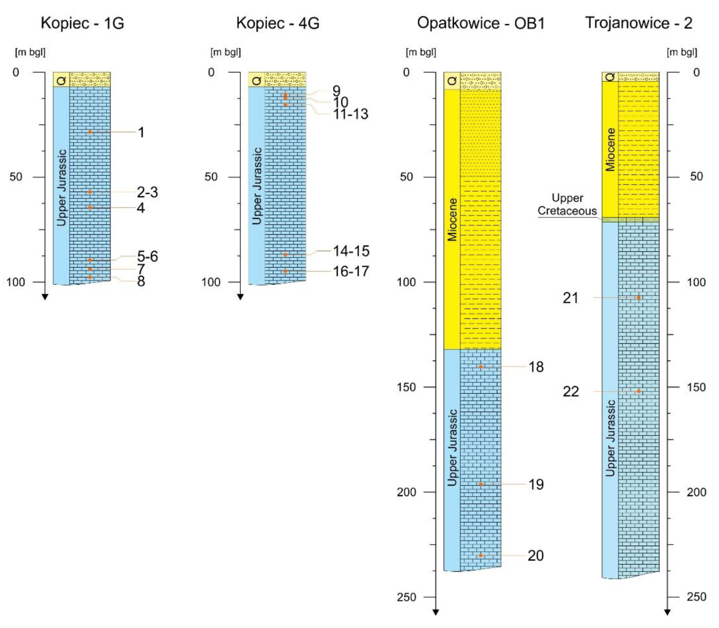
The investigations were conducted on 22 rock samples collected from four boreholes in the Kraków region: Kopiec-1G, Kopiec-4G, Opatkowice-1, and Trojanowice-2 (Figure 2 and Figure 3).
All of the samples represent limestones of the Upper Jurassic stage. Jurassic carbonate formations represent the main part of the geological profile to 200 m below ground level, especially in the central and north-western part of Kraków.
Rock samples were collected during the realization of the GeoPLASMA-CE “Shallow Geothermal Energy Planning, Assessment and Mapping Strategies in Central Europe” project carried out in 2016–2019. The project aimed at encouraging shallow geothermal use in heating and cooling strategies in central Europe. Within the GeoPLASMA-CE project, only thermal conductivity measurements of dry samples were conducted. The methods and the range of the measurements undertaken in the current study exceeded the scope of the above-mentioned project. The thermal conductivity values for both dry and saturated samples, and the quantitative mineral composition and porosity, were determined for all rock samples. To address the large heterogeneity of the pore space (unequal distribution of vugs and fractures), computed tomography was used for the selection of samples suitable for particular investigations (Figure 4).
Several laboratory methods allow for the determination of thermal conductivity values. These can be divided into two groups: steady-state methods and transient techniques. Selection of a laboratory method for thermal conductivity determination should be based on the characteristics of the tested material, namely thermophysical properties of the sample, and the quantity and form of the supplied material, i.e., powdery or solid sample. Limitations of each of the methods should also be taken into consideration. Transient methods make it possible to obtain results in a shorter time, and steady-state methods require a longer measurement period and a large sample [43]. Due to frequent unequal distribution of vugs and fractures in the pore space, it is difficult to determine the thermal conductivity of carbonate rocks. Hence, if the pore space heterogeneity is to be considered, the measurements of such rocks should be conducted using samples that are as large as possible. The measurements of the investigated carbonates were conducted with the steady-state method by determining the size of the heat flow through the sample using a FOX 50 LaserComp apparatus. The tests were carried out on samples in the shape of slices of 5 cm diameter and 1.5 cm thickness. The mean temperature was 25 °C, and the difference between the heating and the cooling plates was 20 °C, with 5% accuracy. The measurements were conducted on dry samples (samples dried for 12 h in 105 °C) and saturated (water saturation) samples.
Grain density was determined using the helium pycnometry method with a Micrometrics (USA) AccuPyc 1330 apparatus. Bulk density was determined using the mercury displacement method. The porosity value was determined based on density measurements. The mineral content analysis was undertaken with the quantitative X-ray method based on the Rietveld technique [44] using a Panalytical (United Kingdom) X’Pert Pro X-ray diffractometer. The specific heat measurements were made using the differential scanning calorimetry method (TG-DSC) with a Netzsch (Germany) STA 449 F3 Jupiter thermal analyzer. Computed tomography investigations were conducted using a Geotek (United Kingdom) RXCT (Rotating CT system). The mercury injection capillary pressure (MICP) data were collected on a Micromeritics AutoPore IV 9520 device (USA) MICP analysis allows measurement of pore sizes from about 3.5 to 500 μm and provides a number of petrophysical parameters, e.g., pore size distribution, porosity, permeability, skeletal and apparent density, and specific surface area of a sample.
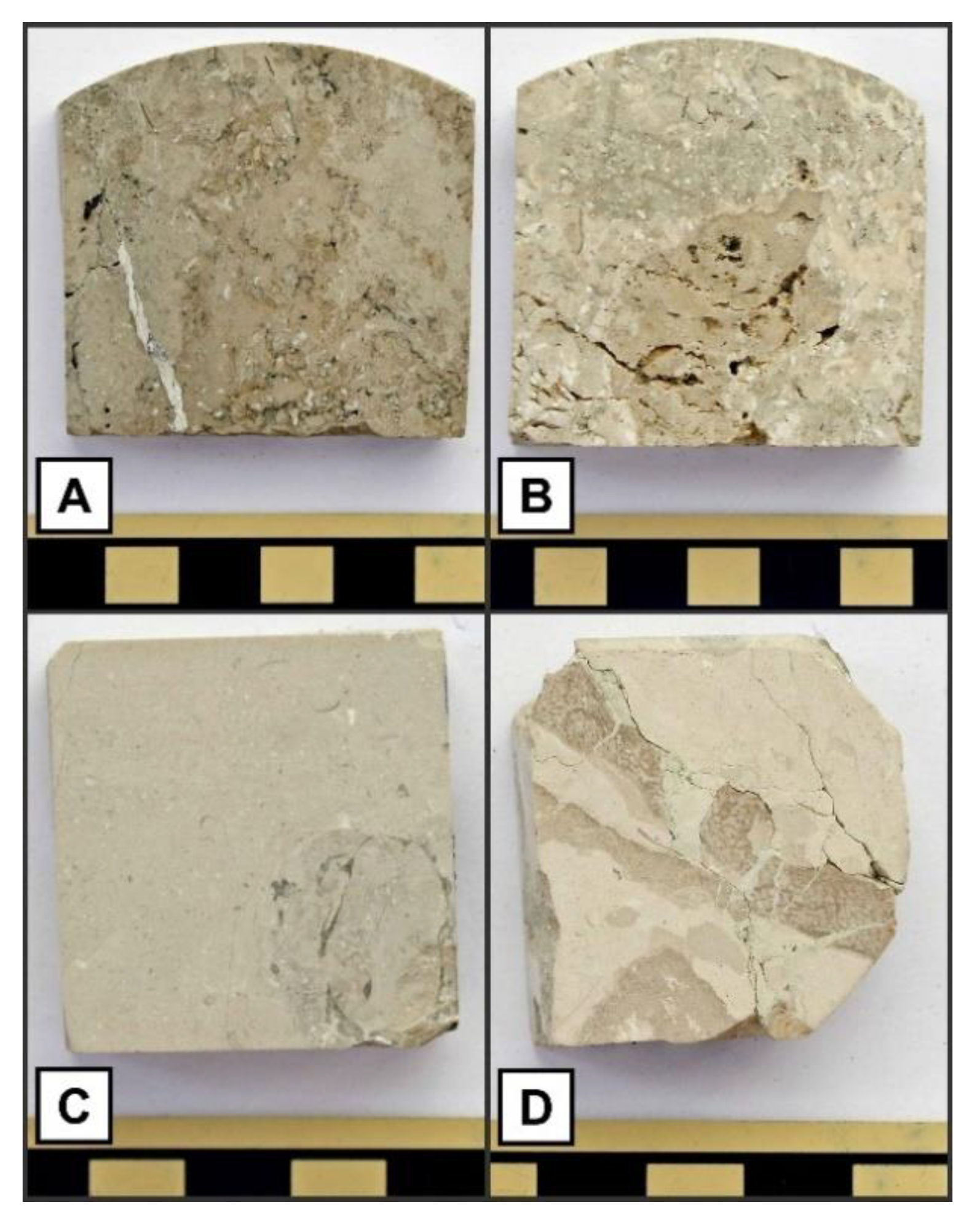
Investigated rocks were microbial-sponge, organodetritical limestones from Kopiec-1G and Kopiec-4G boreholes, and pelitic limestones from Opatkowice-OB1 and Trojanowice-2, representing a series of detrital sponge limestones [45].
Organodetritical limestones from Kopiec-1G and Kopiec-4G (Figure 5A,B) have beige, grey–beige, and grey hues with visible microbial and sponge structures also containing fragments of bivalvia, brachiopoda, and bryozoa. In several samples of stylolites, selective dolomitization and recrystallization processes were observed.
The samples from Opatkowice-OB1 and Trojanowice-2 (Figure 5C,D) were represented by pelitic limestones with grain elements of beige and grey-beige hues, and sponges and bryozoa were visible in some places.
The mineral composition of limestones was minimally diversified (Table 3); the dominant mineral was calcite, and its content generally exceeded 99%. Quartz appeared in small amounts (below 1–2%) in most rocks. Only in samples 6 and 18 were high amounts of quartz—95.6% and 35.2%, respectively—found due to the presence of silificated sponges. In several rocks, dolomite admixtures (from 1.5% to 8%) were present, most likely connected with selective dolomitization processes.
The investigated rocks were characterized by highly diversified porosity of 1.63% to 12.14% (Table 3). The lowest porosity value (below 2%) was found in sample 3 from Kopiec-1G and in samples 16 and 17 from Kopiec-4G, in which recrystallization processes were observed. Samples 11–13 from Kopiec-4G, and 21 and 22 from Trojanowice-2, possessed the highest (above 10%) porosity values. In these rocks, large, usually connected to sponges (Figure 5B,D), vugs were macroscopically visible. Such vugs are described as primary porosity [46,47].
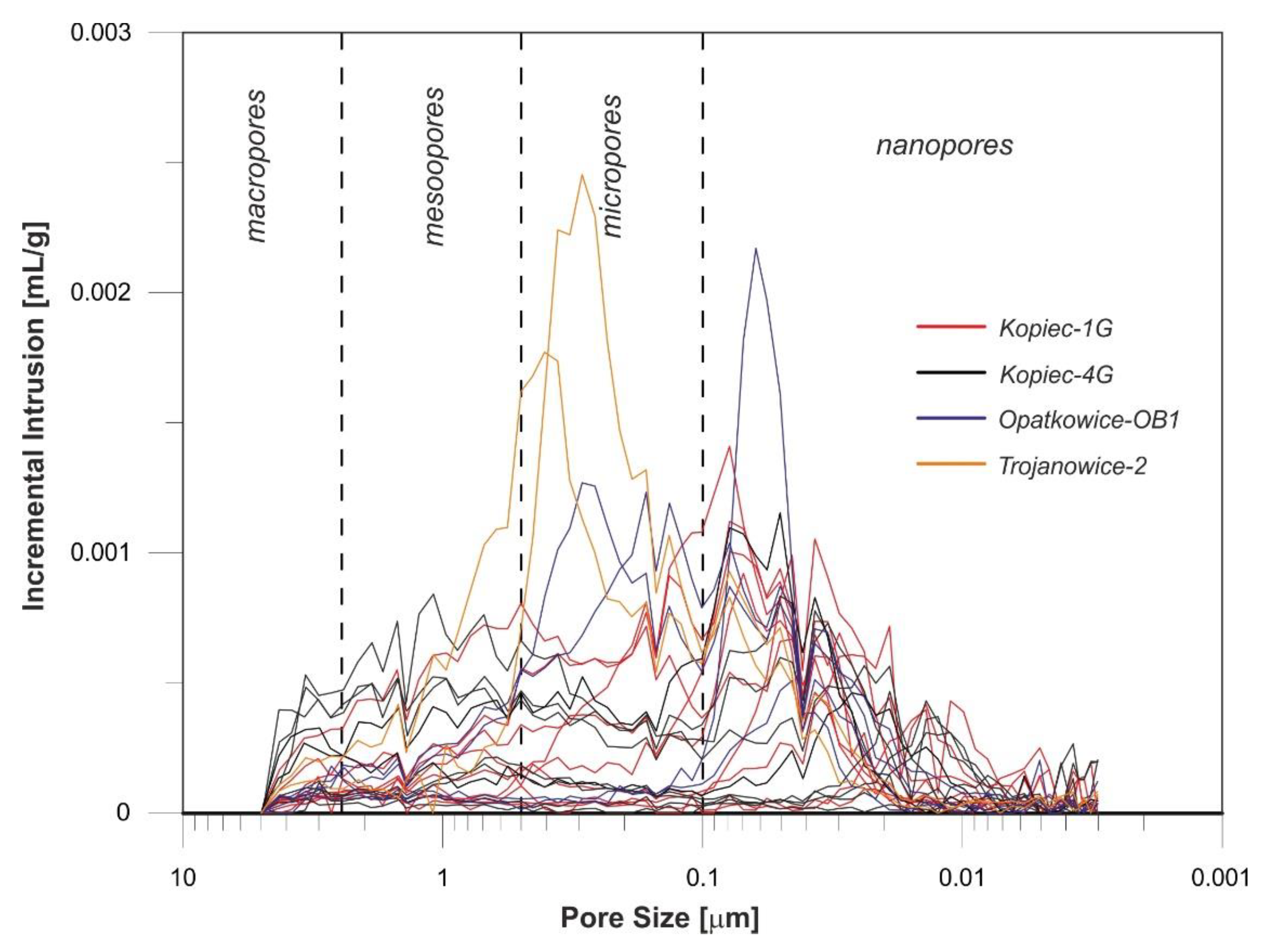
The results of investigations conducted with the MICP method verified the fractured and vuggy character of the pore space.
Figure 6 shows both the cumulative intrusion curves obtained from MICP tests and the pore size distribution. The incremental intrusion curves (Figure 6) represent the pore volume accessed through pore throats of a given size [48,49]. Assessment of the pore space geometry in the studied carbonates indicates the porous-fracture type of the reservoir space, which is mainly unimodal in nature. Pore size classification is based on the grading proposed by Hartmann and Beamont [50]. The dominant pore systems for the studied samples occur in the pore size diameter range of 0.02–5 μm. This indicates that the pore space corresponds mainly to micro- and nanopores (Figure 6, Table 4). The relationship between the pore space formation, porosity, and thermal conductivity is most visible in the carbonate rock samples from Trojanowice-2. These are samples with dominant micropores (Figure 6), followed by high porosities obtained both by MICP and helium methods (Table 3 and Table 4). The share proportion of particular pore types is the main factor conditioning the obtained different results of thermal conductivity of the analyzed samples. The differences in the porosity results obtained by helium and MICP methods are due to different measurement ranges of these methods [51], in addition to the measurement methodology. In the case of MICP, measurement is carried out using crushed samples, thus eliminating big pores and fractures, thus decreasing the porosity.
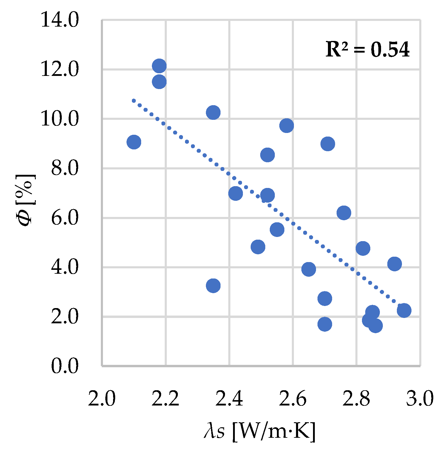
Thermal conductivity coefficient values λ for dry samples range from 1.69 to 2.76 W/m∙K, and for saturated samples from 2.10 to 2.95 W/m∙K (Table 3, Figure 7). Low TC values are generally reflected by high porosity (Table 4). A distinctive decrease in thermal conductivity values in line with increasing porosity (Table 3, Figure 8 and Figure 9) is observed in regards to both the dry and saturated samples. Heat capacity values (specific heat) range from 0.889 to 0.924 J/g K (Table 5).

6. Mathematical Models

The mathematical models noted previously were used to compute the thermal conductivity of the investigated samples. Calculations were carried out for 22 carbonate rocks from the Kraków region. All analyses were performed on saturated samples.
The analyses were carried out using the following procedure:
  • Determination of the thermal conductivity of all samples using arithmetic, harmonic, and geometric means and comparing them with the laboratory measured conductivities (Figure 10);
  • Removal of two outstanding samples of different mineral composition (high content of quartz) from the applied models (Figure 11) and correlation analysis of obtained results (Figure 12);
  • Applying the models to samples divided into two groups: of porosity higher and lower than 4% (Figure 13), and correlation analysis of obtained results (Figure 14);
  • Determining the thermal conductivity using spherical inclusion models (Clausius–Mossotti) (Figure 15 and Figure 16), taking into consideration the division of samples into two groups of different porosity (Figure 17) and correlation analysis of obtained results (Figure 18);
  • Thermal conductivity determination of all samples using non-spherical inclusion models (Figure 19 and Figure 20) taking into consideration the division of samples into two groups of different porosity (Figure 21) and correlation analysis of obtained results (Figure 22);
  • Introducing a correction allowing for approximation of the modelled values (Figure 23) to the laboratory measured values (Figure 24, Figure 25, Figure 26, Figure 27, Figure 28, Figure 29, Figure 30 and Figure 31).
The thermal conductivity of the rock matrix used in the applied models was calculated based on the content and thermal conductivity of minerals (Table 1). The content (percentage by weight) of minerals was obtained using XRD analysis (Table 3) and converted into volume percent.

6.1. Layer Models and Geometric Mean

The layer (λ_arytm and λ_harm) and geometric mean (λ_geom) models were compared with laboratory measurements for all investigated samples (Figure 10).
A distinct influence of mineral composition on matching calculated to measured thermal conductivity values was observed. Two rocks (samples 6 and 18, indicated with a red ellipse in Figure 10) are characterized by overestimated values that are distinct from others. These samples contain significantly higher amounts of quartz (35% and 95%) than other rocks (maximum 2.5%). Regarding different mineralogy, they were excluded from further consideration.
Comparison of λ_arytm and λ_harm (Figure 11) with laboratory measurements verified the theoretic assumption: the highest values are indicated by λ_arytm (the model assuming the heat flowing parallel to the boundary between components) and the lowest by λ_harm (the model assuming the heat flowing perpendicular to the boundary between components). The values obtained based on the λ_geom model are similar to those of λ_harm (Figure 11). Each of the three models overestimated results in regard to the laboratory measured values and displayed medium correlation factors (Figure 12a–c). Then, the set of data was divided into two subgroups: samples of porosity above 4% (Figure 13a) and samples of porosity below 4% (Figure 13b). Two samples characterized by calculated thermal conductivity values that differed most from laboratory measurements (samples 8 and 10, Figure 11 and Figure 13a) were excluded from the group of higher porosity samples. This procedure allowed considerably better correlations for rocks of porosity higher than 4% to be obtained compared to the whole set of samples (Figure 14). The best correlation coefficient (R2 = 0.72) is characteristic for λ_geom (Figure 14b) and the calculated values are most similar to the measured values for λ_harm (Figure 14c). The values obtained by each of the three models for samples of porosity lower than 4% are significantly overestimated (Figure 13b) and do not correlate with the measured values.

6.2. Clausius–Mossotti Spherical Inclusions Model

In the next step, the Clausius–Mossotti spherical inclusion models were tested [12]. Both of the applied models λ_sph_m (rock composed of a grain matrix and pores in the shape of spherical inclusions) and λ_sph_f (rock composed of spherical grains dispersed in a pore solution) show that thermal conductivity values are overestimated in relation to the measured values (Figure 15). Similarly, as in the case of the layer and geometric mean models (Figure 12 and Figure 14), the correlations carried out for the whole collection of samples (Figure 16) improve after distinguishing a subgroup of samples of porosity above 4% (Figure 17 and Figure 18). In that group, the λ_sph_f model yields values most similar to the measurements.

6.3. Non-Spherical Inclusion Models

For models assuming pores of ellipsoid shapes, extreme cases of elongated, needle shaped pores (λ_nsph_n), pores of spherical shape (λ_nsph_s), and disk-shaped pores (λ_nsph_d) were analyzed (Figure 19). Similar results were obtained for λ_nsph_s (counterpart of spherical inclusion model λ_sph_m) and λ_nsph_n models (Figure 19).
Model λ_nsph_d gave slightly lower values that were more similar to the measured values. As in the case of other models, significantly better correlations were obtained for the distinguished subset of samples of porosity above 4% (Figure 21 and Figure 22) than for all of the rocks (Figure 20).

7. Analysis of the Obtained Results

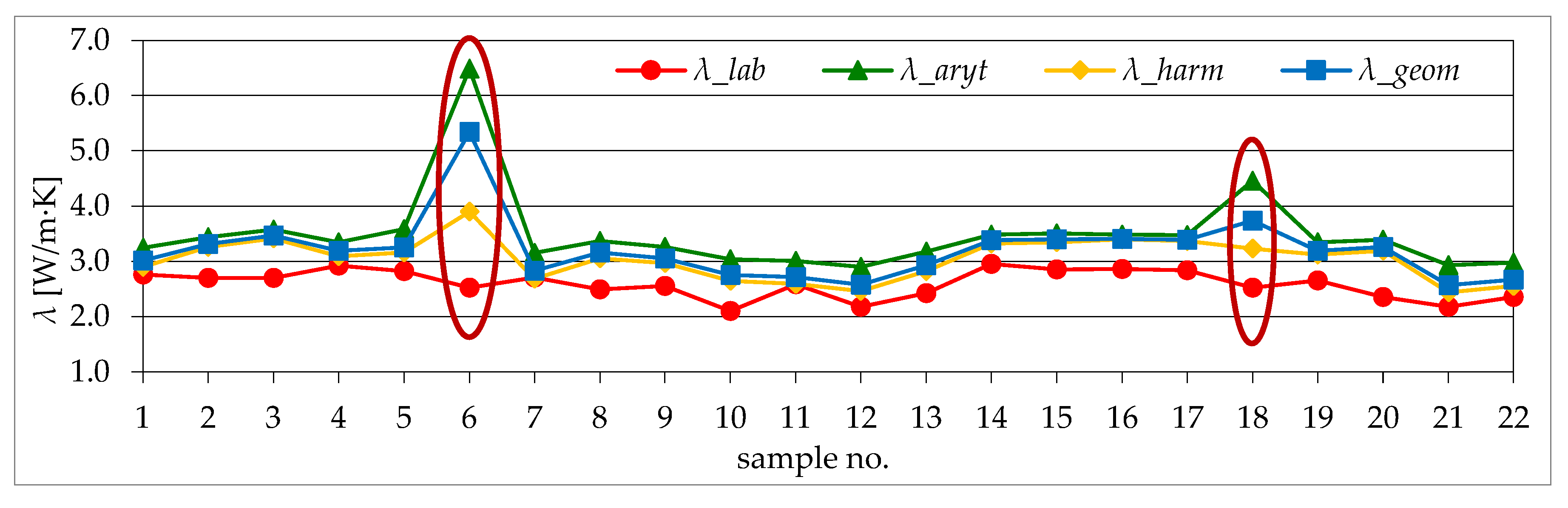
The comparison of the laboratory measured thermal conductivity values with those obtained by mathematical models clearly indicates the impact of both the mineralogy and petrophysical properties of the investigated rocks on the models tested. The influence of mineralogy is visible in the case of two samples (samples 6 and 18) with outstandingly high quartz content (Figure 10). These samples are characterized by the distinctively different from the other ones, overestimated thermal conductivity values obtained from layer and geometric mean models. As mentioned previously, these samples were excluded from further considerations. Another highly important factor is porosity. Two groups of samples of different pore space geometry—compact rocks of low porosity and vuggy samples of porosity above 4%—were distinguished in the set of the investigated rocks. Considerably better correlation coefficients (R2 = 0.69–0.74) were obtained for rocks of porosities above 4% than for the whole set of samples (R2 = 0.55–0.59). The overestimated values obtained in the result of calculations are probably due to understated porosity values caused by the appearance of isolated pores, which are not reflected in the laboratory measurements. The influence of lithology on the calculated thermal conductivity values was also observed for siliciclastic rocks [21,22].
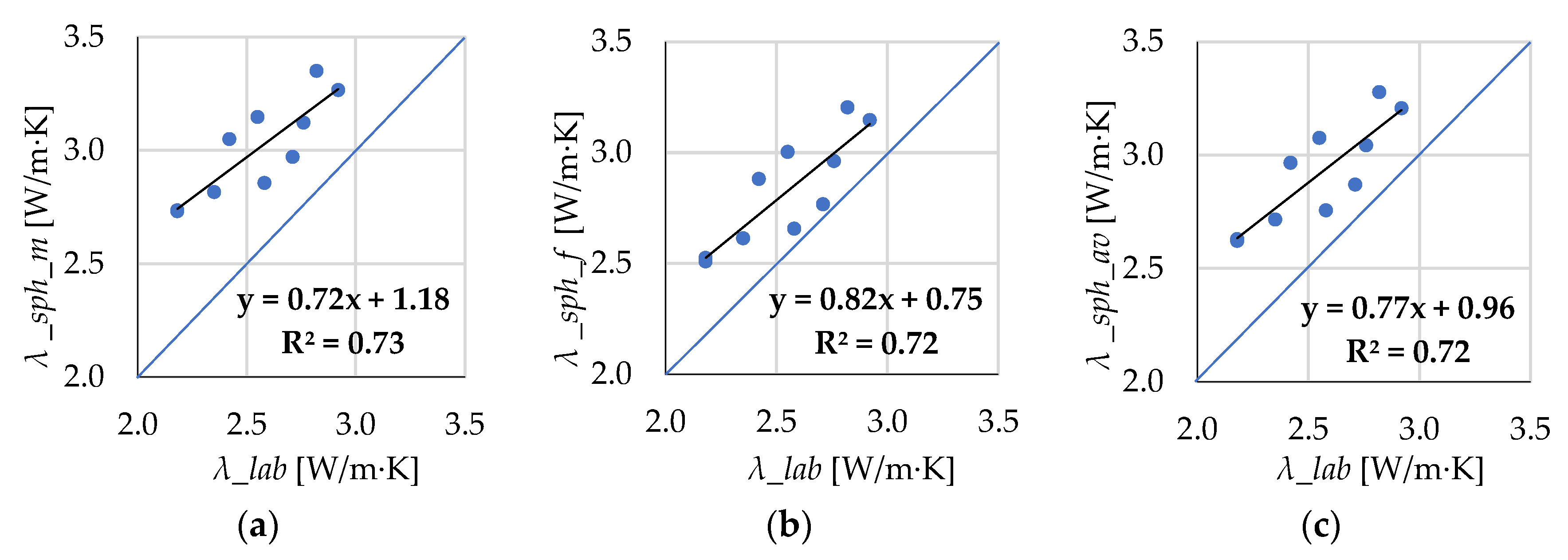
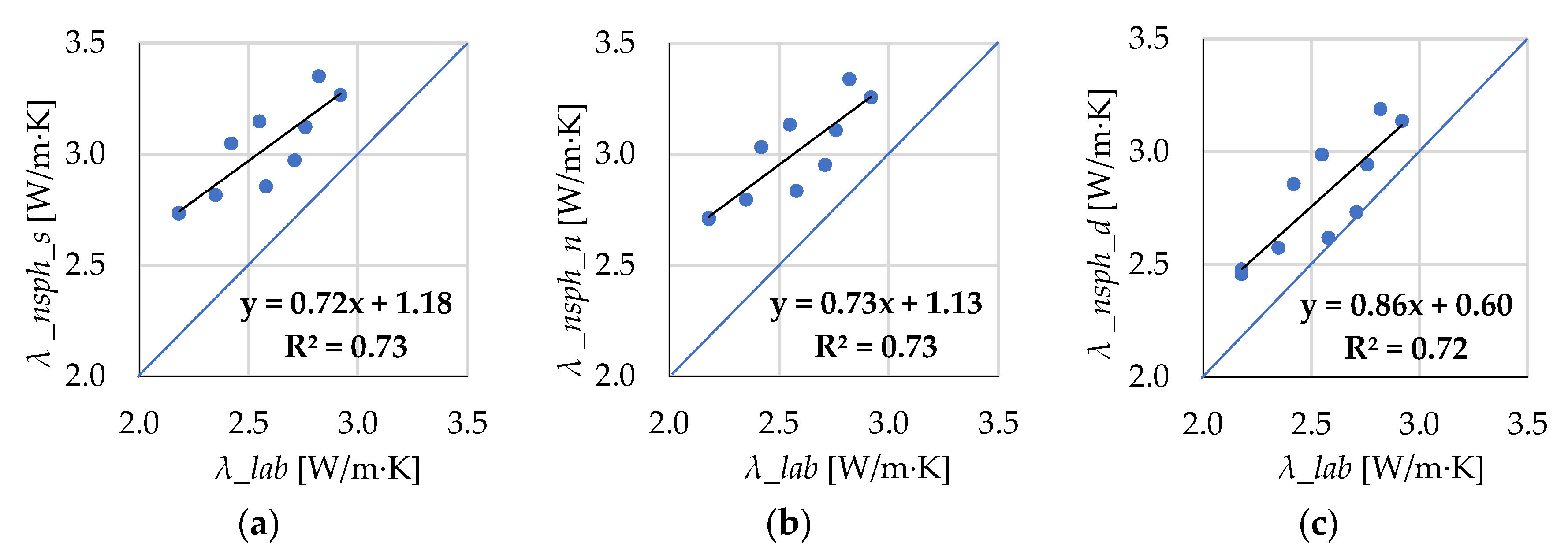
Comparison of all of the models calculated for the subgroup of rocks of porosity over 4% (Figure 23) allowed the models that best fit the laboratory measurements to be identified.
As shown in Figure 23, the best conformity of results was obtained for models λ_harm, λ_sph_f, and λ_nsph_d. Each of the three models assume a structure of the pore space in which the contacts between the framework grains are limited. As described above, model 
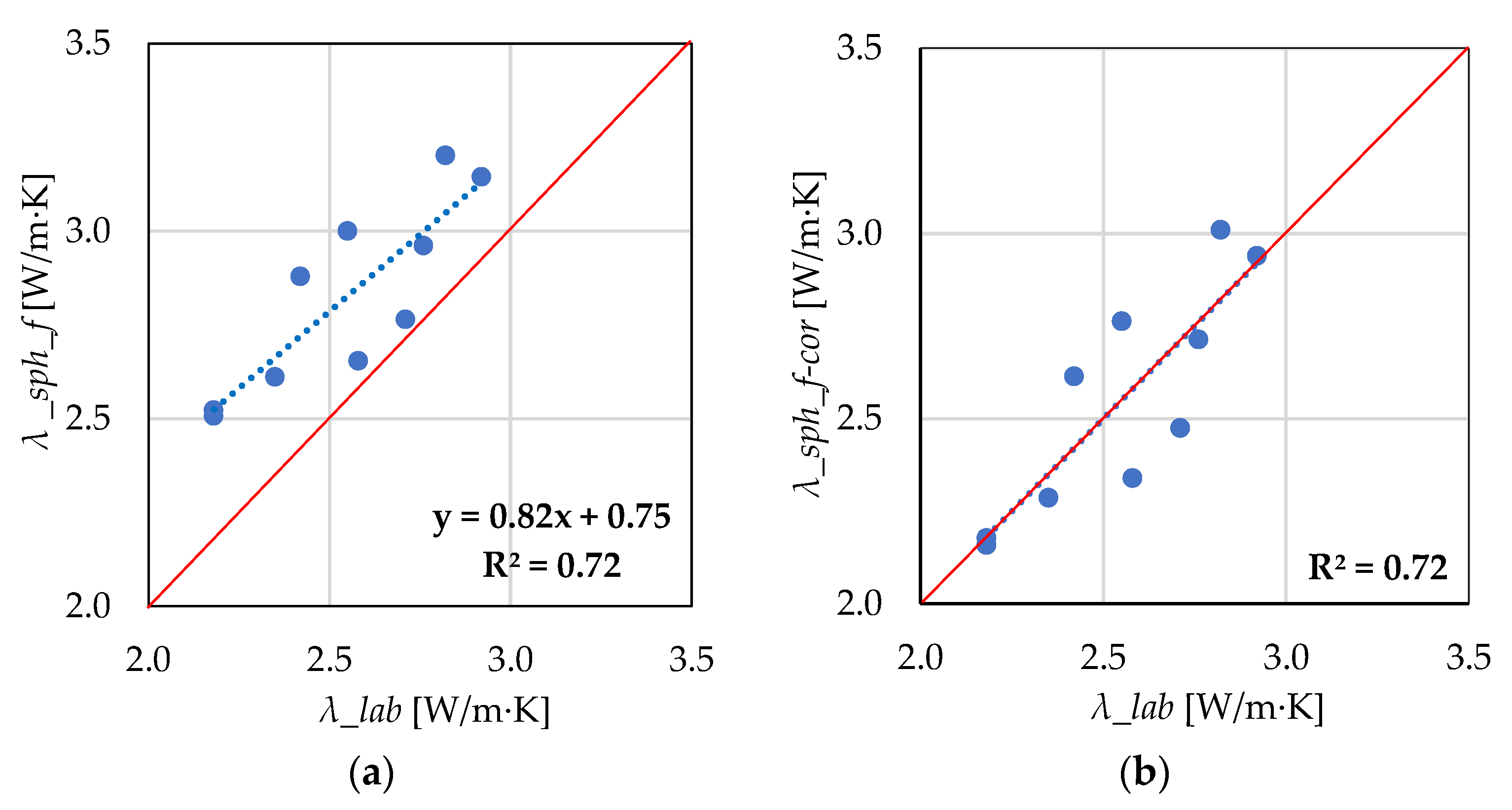
λ_sph_f is that of rock composed of spherical grains dispersed in the pore solution, model λ_nsph_d is characterized by the presence of extended fractures, whereas model λ_harm assumes the heat flow perpendicular to the layers consisting of respective components of the rock (including pore solutions). It appears that these theoretic assumptions can be applied to rocks where porosity is connected to unequally distributed and sometimes large vugs filled with gas or brines constituting “a barrier” against the heat flow.
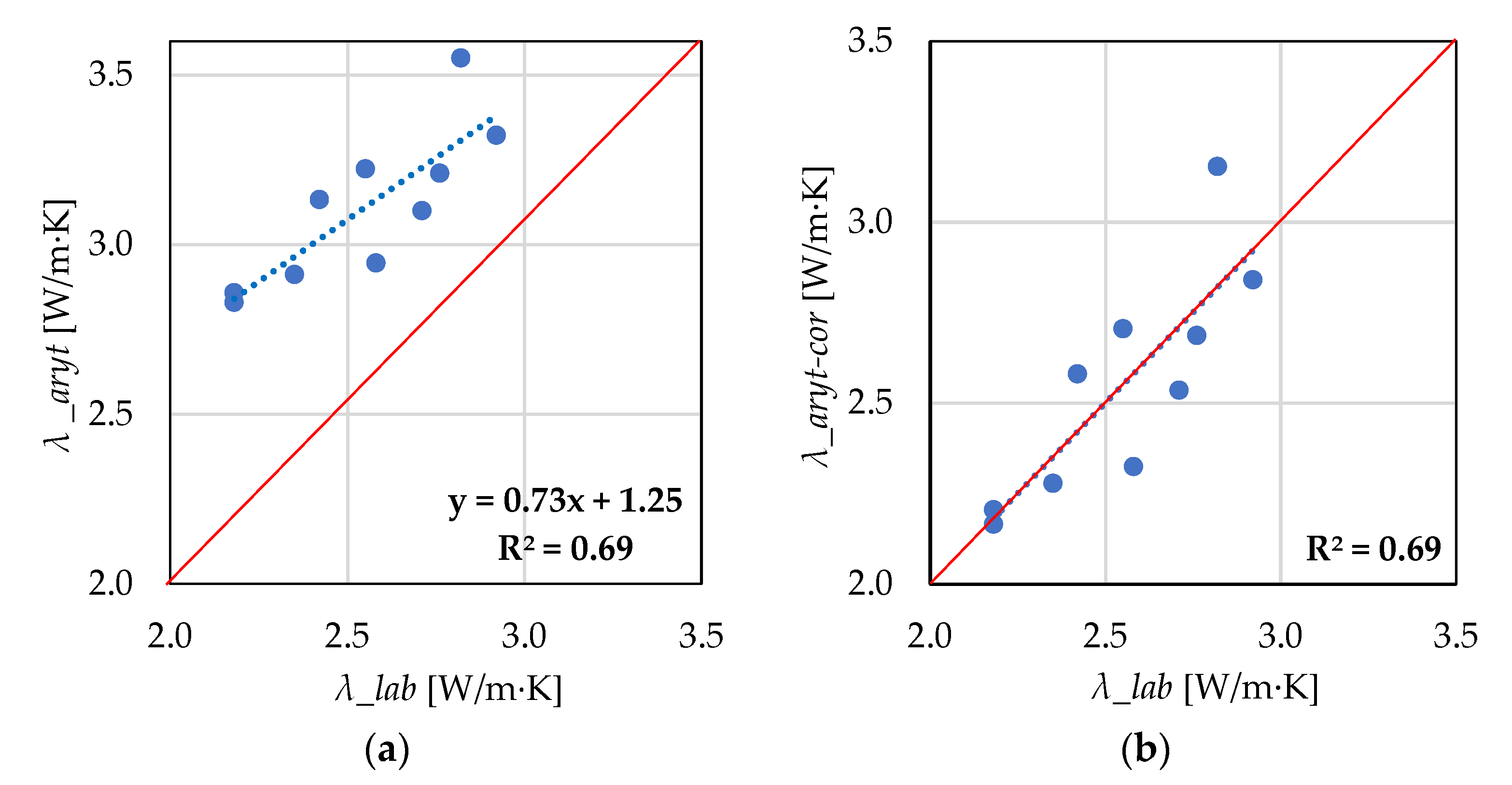
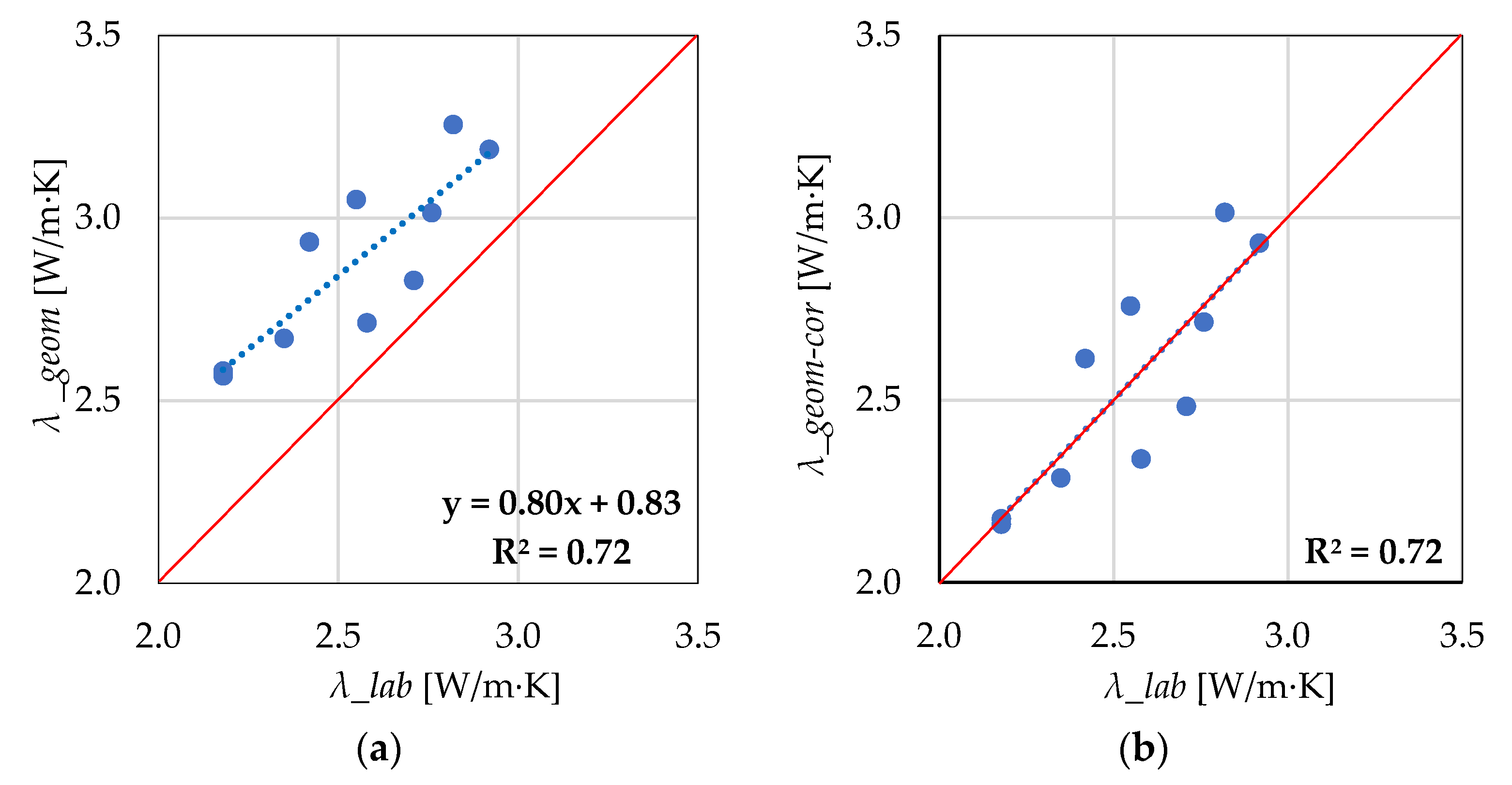
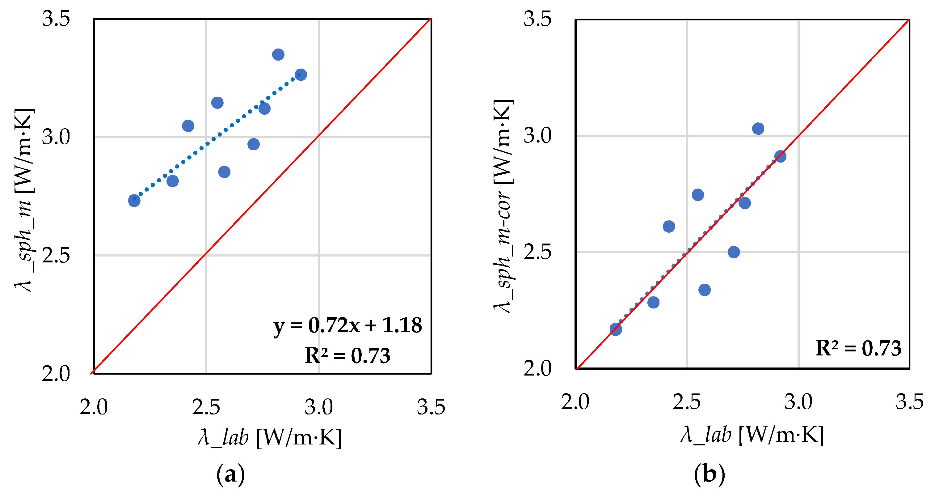
A correction allowing for the approximation of values obtained by the models to the laboratory measured values was applied. Such a correction can be introduced when the correlation between the calculated and measured values is of sufficient quality. The obtained linear equations showing relationships between the calculated models and the laboratory measurements were used, and calculations were made for each of the models (Table 6).
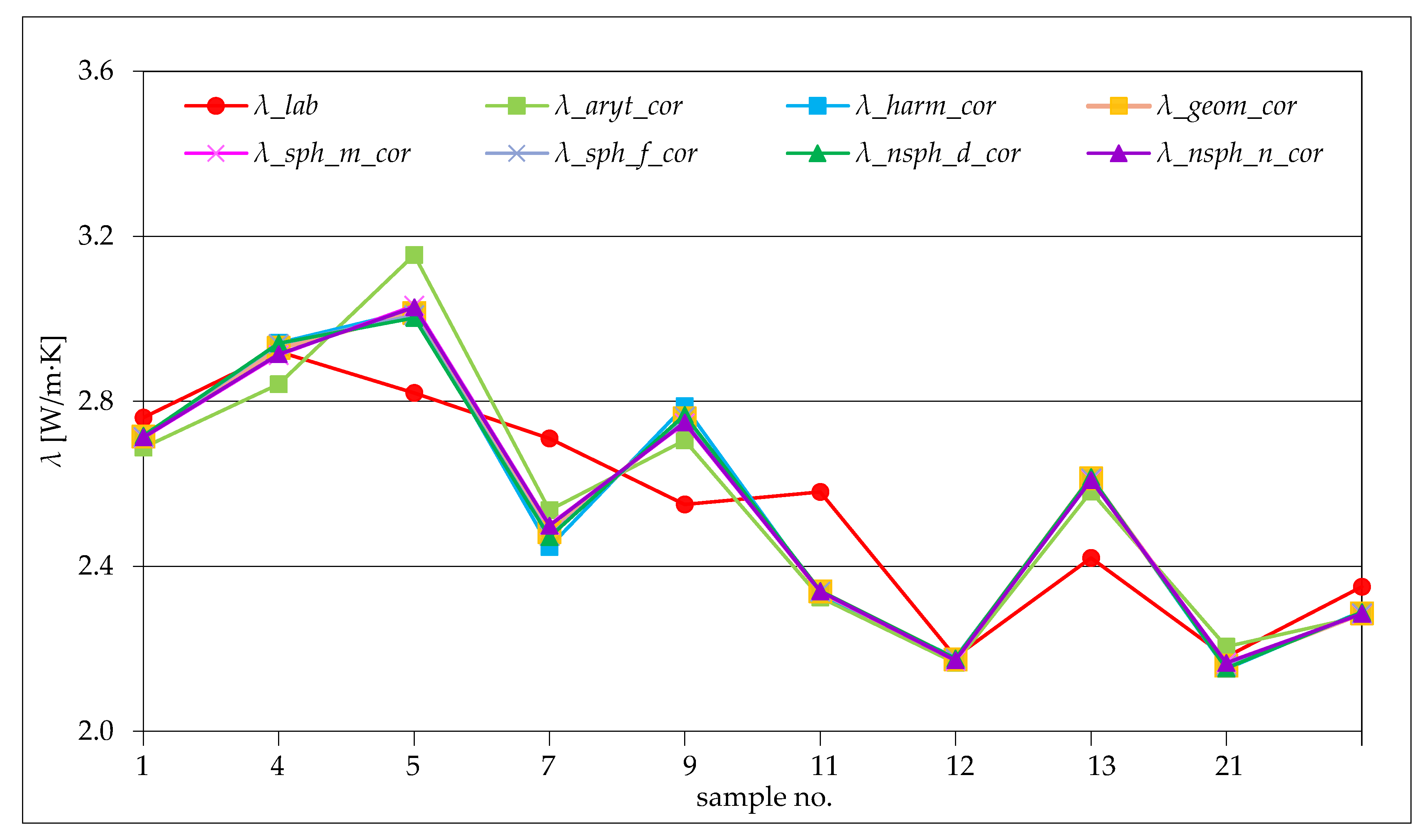
In each case, the corrected thermal conductivity values are considerably closer to the laboratory measurements (Table 7, Figure 24, Figure 25, Figure 26, Figure 27, Figure 28, Figure 29, Figure 30 and Figure 31) than the uncorrected values. An attempt to select the best models using an analysis of differences between the measured thermal conductivity values and the corrected values was undertaken. The analysis showed that λ_aryt and λ_harm models are the least useful for introducing the correction (Figure 31). The remaining models do not differ significantly. It should be mentioned that the solutions obtained for 10 samples must be treated as preliminary. To verify the results, a higher number of samples should be tested.

8. Summary and Conclusions

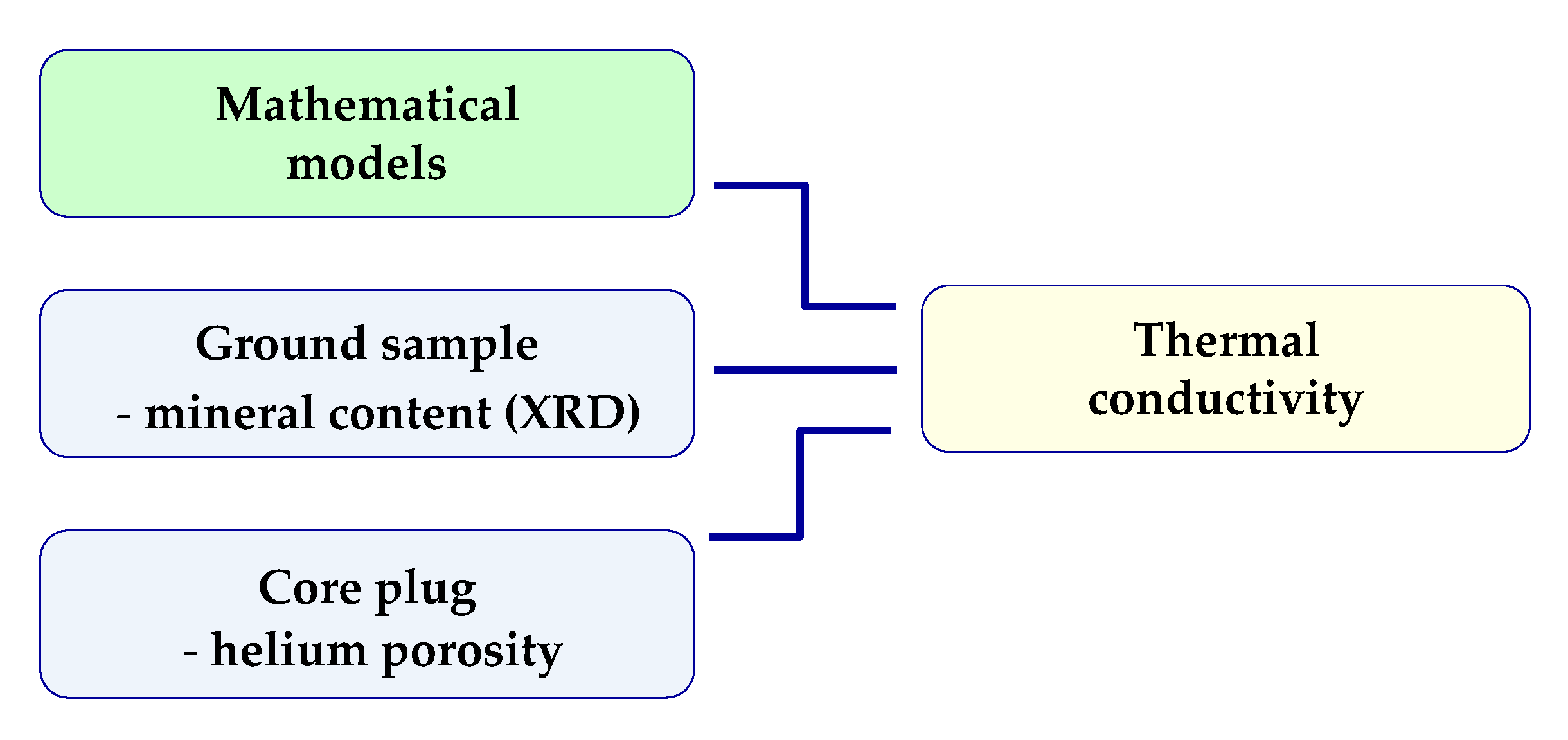
A method using mineralogical, petrophysical, and thermal data to determine the thermal potential of carbonate rocks from the Kraków region was introduced. Analyses of mineral composition, porosity, and thermal conductivity were conducted, and the thermal conductivity coefficient was assessed using mathematical models. The proceedings followed the investigation scheme presented in Figure 32.
The obtained model allows the thermal conductivity database to be extended in cases where it is not possible to measure this parameter due to a sparse amount of rock material.
Due to computed tomography measurements, it was possible to depict the inner structure and to trace the distribution of fractures and vugs in the investigated limestones. These also allowed representative core fragments to be chosen for thermal conductivity and porosity measurements. It is particularly important in the case of rocks with high variability of the pore space, such as the investigated limestones. The tomography image clearly shows that porosity is related to unevenly distributed, sometimes large vugs and fractures which constitute a “barrier” against the heat flow. The best match of the measured and calculated results was obtained by the models that assumed such a structure of the pore space, in which the grain contacts of the framework are limited by either the advantage of pore solutions over the framework grains (λ_sph_f) or the presence of extended voids (λ_harm and λ_nsph_d).
Mineral composition investigations were essential in the construction of mathematical models, taking into consideration the volume of particular minerals with appropriate thermal conductivity coefficients. These measurements also made it possible to analyze the influence of mineralogy on the calculated models. As a result of the analysis, two samples (samples 6 and 18) of different mineral composition (high amounts of quartz) were excluded from the input data.
An analysis of porosity measurements proved the dominant influence of porosity on the thermal conductivity value and allowed the measurement data to be arranged to obtain the best fitting of the tested models. In most cases, the calculated thermal conductivity values were overestimated compared to the laboratory measured values. This was probably due to the presence of isolated pores that was not reflected in the laboratory measurements of porosity. This was confirmed by the considerably better conformity of results for all investigated models obtained for a selected subgroup of samples of porosity exceeding 4% (R2 from 0.69 to 0.74) than for all samples (R2 from 0.55 to 0.59).
Using the good correlation coefficients obtained for the group of rocks of porosities above 4%, a correction was made so that the calculated values approximated the measured thermal conductivities. The calculation of thermal conductivity based on both mineral composition and porosity (Figure 33) is essential for completing the thermal database of carbonate rocks in the investigated region. As mentioned, the amount of material from a number of boreholes is too sparse to conduct laboratory measurements of thermal conductivity, and samples from outcrops are often weathered.
Thermophysical rock properties are key parameters for the assessment of shallow geothermal resources, future design of geological work, effective heat/cold extraction, and sustainable resource management. From the study of the thermo- and petrophysical properties of the carbonate rocks in the Kraków area, the following conclusions can be drawn:
  • The studied Upper Jurassic rocks are a heterogenous formation of limestones, which can be differentiated in structure and fabric. These differences affect the thermo- and petrophysical properties of the rocks and show related trends;
  • Thermal conductivity was assessed by means of mathematical models based on a simplification of the rock’s structure, allowing for calculation of the rock thermal conductivity based on the properties of its components;
  • The best correlations between calculated and measured thermal conductivity values (R2 from 0.69 to 0.74) were obtained for the subgroup samples of porosity higher than 4%. The subgroup of samples of porosity lower than 4% did not show a satisfactory fit of data and was not taken into consideration in the subsequent analyses;
  • The models which yielded values most approximate to the laboratory measurements were λ_harm, λ_sph_f, and λ_nsph_d;
  • A correction based on the obtained linear equations showing relationships between the respective calculated models to the laboratory measurements was introduced. The corrected thermal conductivity values were considerably closer to the laboratory measurements;
  • The developed measurement workflow allows for the use of mineralogical and petrophysical analysis to identify the geothermal potential of carbonate rocks;
  • Calculated mathematical models of thermal conductivity provide information on the main factors controlling this property. This will enable selection of optimal rock parameters in the design phase of a shallow geothermal installation;
  • The proposed methodology appears to be justified for the case in which a reliable set of data is used to verify mathematical models of thermal conductivity of carbonate rocks. In particular, the discussed methods and models can be used to refine existing geothermal potential maps or calibration of 3D parametric models used to design prognostic calculations of technical installations for shallow geothermal energy use.
The preparatory research for this article, combined with the established methodology for estimating the thermal conductivity of carbonate rocks in the Kraków area, is the first stage of our work, which will most likely be continued by our team in the future.

Author Contributions

Conceptualization: M.H. and A.P.; formal analysis: A.P., G.M. and K.D.; methodology: A.P., K.D. and G.M.; resources: M.H., A.P., G.Z. and G.M.; supervision: M.H. and A.P.; visualization: A.P., K.D. and G.Z.; writing—review and editing: M.H., A.P., G.M., K.D. and G.Z. All authors have read and agreed to the published version of the manuscript.

Funding

This research was funded by statutory research program at the Faculty of Geology, Geophysics and Environmental Protection AGH University of Science and Technology in Krakow, Poland, statutory work No. 16.16.140.315 as well as Oil and Gas Institute—National Research Institute in Krakow, statutory work No. 53/SW/19.

Acknowledgments

We would like to thank Andrzej Urbaniec for his help in the macroscopic description of the investigated limestone samples.

Conflicts of Interest

The authors declare no conflict of interest.

Terminology and Abbreviations

TCthermal conductivity
CTcomputed tomography
BHEborehole heat exchanger
TRTthermal response test
GSHPground source heat pump
λmthermal conductivity of the grain framework
λfthermal conductivity of the pore media
ϕ porosity
Vvolume fraction of the inclusions
λthermal conductivity of the whole rock
λ1thermal conductivity of the inclusion material
λ2thermal conductivity of the host material
λ_lablaboratory measured thermal conductivity of saturated sample
λ_arytthermal conductivity calculated by applying arithmetic mean (Equation (1))
λ_harmthermal conductivity calculated by applying harmonic mean (Equation (2))
λ_geomthermal conductivity calculated by applying geometric mean (Equation (6))
λ_sph_mthermal conductivity calculated by applying spherical inclusion models, for rock consisting of grain framework and pore solutions appearing as spherical inclusions (Equation (4))
λ_sph_fthermal conductivity calculated by applying spherical inclusion models, for rock consisting of spherical grains suspended in a fluid (Equation (5))
λ_sph_avthermal conductivity calculated by applying spherical inclusion models, average value
λ_nsph_sthermal conductivity calculated by applying non-spherical inclusion models, case α→1, pores of the sphere shape (Equation (7))
λ_nsph_nthermal conductivity calculated by applying non-spherical inclusion models, case α→∞, pores of the needle shape (Equation (7))
λ_nsph_dthermal conductivity calculated by applying non-spherical inclusion models, case α→0, pores of the disk shape (Equation (7))
λ_aryt-corcorrected thermal conductivity value, calculated by applying arithmetic mean
λ_harm-corcorrected thermal conductivity value, calculated by applying harmonic mean
λ_geom-corcorrected thermal conductivity value, calculated by applying geometric mean
λ_sph_m-corcorrected thermal conductivity value, calculated by applying spherical inclusion models, for rock consisting of grain framework and pore solutions appearing as spherical inclusions
λ_sph_f-corcorrected thermal conductivity value calculated by applying spherical inclusion models, for rock consisting of spherical grains suspended in a fluid
λ_nsph_n-corcorrected thermal conductivity value calculated by applying non-spherical inclusion models, case α→∞, pores of the needle shape
λ_nsph_d-corcorrected thermal conductivity value calculated by applying non-spherical inclusion models, case α→0, pores of the disk shape

References

  1. Renewables 2019 Global Status Report. A Comprehensive Annual Overview of the State of Renewable Energy. Global Carbon Project. Available online: https://www.ren21.net/wp-content/uploads/2019/05/gsr_2019_full_report_en.pdf (accessed on 19 January 2020).
  2. Eurostat 2019. Dane Statystyczne Dotyczące Energii ze Źródeł Odnawialnych. Available online: https://ec.europa.eu/eurostat/statistics-explained/index.php?title=Renewable_energy_statistics/pl (accessed on 19 January 2020).
  3. Garabetian, T.; Dumas, P.; Serrano, C.; Pinzuti, V.; Mazzagatti, V.; Kumar, S.; Dimitrisina, R.; Ruaud, J.; Truong, C. EGEC Geothermal Market Report—Full Report, 8th ed.; EGEC—European Geothermal Energy Council: Brussel, Belgium, 2019; p. 61. [Google Scholar]
  4. Global Carbon Project. Available online: https://www.globalcarbonproject.org/carbonbudget/19/files/GCP_CarbonBudget_2019.pdf (accessed on 19 January 2020).
  5. Minister Aktywów Państwowych. Krajowym Planie na Rzecz Energii i Klimatu na Lata 2021–2030. Available online: https://www.gov.pl/web/aktywa-panstwowe/krajowy-plan-na-rzecz-energii-i-klimatu-na-lata-2021-2030-przekazany-do-ke (accessed on 19 January 2020).
  6. Polish Emission Standards for Domestic Boilers—Ecodesign PN-EN 303-5: 2012. p. 82. Available online: https://tnij.com/r5S (accessed on 19 January 2020).
  7. Anti-Smog Resolution for Kraków 2016. Available online: https://bip.malopolska.pl/umwm/Article/get/id,1159347.html (accessed on 19 January 2020).
  8. Hajto, M.; Ciapała, B.; Ząbek, G.; Michna, M.; Papiernik, B. (Eds.) Reviewed Strategies for the Use of Shallow Geothermal Energy in the Investigated Pilot Areas—Kraków; GeoPLASMA-CE Project Deliverable D.T4.2.3; Interreg CENTRAL EUROPE Programme Joint Secretariat Kir: Kraków, Poland, 2019; p. 70. [Google Scholar]
  9. Ozimek, J.; Koczorowski, J. Ekspertyza Dotycząca Danych Technicznych i Operacyjnych Instalacji Płytkiej Geotermii, w tym Geotermalnych Pomp Ciepła: Gruntowych Wymienników Ciepła i Instalacji Typu Woda-Woda, Wraz z Analizą Możliwości Wykonania Specjalistycznych Pomiarów TRT w Obszarze Pilotażowym Krakowa; GeoPLASMA-CE Project Deliverable D.T4.2.3; Interreg CENTRAL EUROPE Programme Joint Secretariat Kir: Wrocław, Poland, 2018; p. 15. [Google Scholar]
  10. Lachman, P. Raport Rynkowy PORT PC; Rynek Pomp Ciepła w Polsce w latach 2010–2018. Perspektywy Rozwoju Rynku Pomp Ciepła do 2030 Roku; PORT PC: Kraków, Poland, 2019; p. 46. [Google Scholar]
  11. MPEC SA. Plan Rozwoju MPEC S.A. w Krakowie w Zakresie Zaspokojenia Obecnego i Przyszłego Zapotrzebowania na Ciepło. Wieloletni Plan Rzeczowo-Finansowy Spółki na Lata 2018–2024; MPEC SA: Kraków, Poland, 2019; p. 77. [Google Scholar]
  12. Schön, J.H. Physical Properties of Rocks. Handbook of Petroleum Exploration and Production; Elsevier: Oxford, UK; Amsterdam, The Netherlands, 2011. [Google Scholar]
  13. Gegenhuber, N.; Schoen, J. New Approaches for the Relationship between Compressional Wave Velocity and Thermal Conducticity. J. Appl. Geophys. 2012, 76, 50–55. [Google Scholar] [CrossRef]
  14. Goutorbe, B.; Lucazeau, F.; Bonneville, A. Using neural networks to predict thermal conductivity from geophysical well logs. Geophys. J. Int. 2006, 166, 115–125. [Google Scholar] [CrossRef] [Green Version]
  15. Pimienta, L.X.; Clauser, C.; Klitzsch, N. Comparison of Thermal and Elastic Properties of sandstones: Experiments and Theoretical Insights. Geothermics 2018, 76, 60–73. [Google Scholar] [CrossRef]
  16. Fuchs, S.; Balling, N.; Förster, A. Calculation of Thermal Conductivity, Thermal Diffusity and Specific Heat Capacity of Sedimentary Rocks Using Petrophysical Well Logs. Geophys. J. Int. 2015, 203, 1977–2000. [Google Scholar] [CrossRef] [Green Version]
  17. Hartmann, A.; Rath, V.; Clauser, C. Thermal conductivity from core and well log data. Int. J. Rock Mech. Min. 2005, 42, 1042–1055. [Google Scholar] [CrossRef] [Green Version]
  18. Middleton, M. Determination of Matrix Thermal Conductivity from Dry Drill Cuttings. AAPG Bull. 1994, 76, 1790–1799. [Google Scholar]
  19. Szewczyk, J. Estimation of the heat flow density using thermal parametres modeling. Geol. Rev. 2001, 49, 1083–1088. [Google Scholar]
  20. Zimmerman, R.W. Thermal Conductivity of Fluid-Saturated Rocks. J. Petrol. Sci. Eng. 1989, 3, 219–227. [Google Scholar] [CrossRef]
  21. Przelaskowska, A. Estimating the thermal conductivity value of the Carpathian flysch sandstones on the basis of their mineral composition. Nafta-Gaz 2018, 6, 435–442. [Google Scholar] [CrossRef]
  22. Przelaskowska, A.; Drabik, K.; Klaja, J. Szacowanie wartości współczynnika przewodności cieplnej piaskowców mezozoicznych podłoża Karpat na podstawie składu mineralnego. Geol. Explor. Technol. Geotherm. Energy Sustain. Dev. 2018, 57, 107–121. [Google Scholar]
  23. Blackwell, D.D.; Steele, J.L. Thermal Conductivity of Sedimentary Rocks: Measurement and Significance. In Thermal History of Sedimentary Basins; Naeser, N.D., McCulloh, T.H., Eds.; Springer: New York, NY, USA, 1989. [Google Scholar]
  24. Cermak, V.; Rybach, L. Thermal Properties. In Landolt-Bornstein Numerical data and Functional Relationships in Science and Technology; New, Series; Hellwege, K.-H., Ed.; Group V, Geophysics and Space Research: Berlin, Germany, 1982; Volume 1, pp. 305–371. [Google Scholar]
  25. Gong, G. Physical Properties of Alpine Rocks: A Laboratory Investigation. Ph.D. Thesis, University of Geneva, Geneva, Switzerland, 2005. [Google Scholar]
  26. Jessop, A.M. Thermal Geophysics; Elsevier: Amsterdam, The Netherlands, 1990. [Google Scholar]
  27. Brigaud, F.; Vasseur, G.; Caillet, G. Use of Well Log Data for Predicting Detailed in Situ Thermal Conductivity Profiles at Well Sites and Estimation of Lateral Changes in Main Sedimentary Units at Basin Scale; Rock at Great Depths; Maury, V., Fourmaintraux, D., Eds.; Balkema: Rotterdam, The Netherlands, 1989. [Google Scholar]
  28. Clauser, C.; Huenges, E. Thermal Coductivity of Rocks and Minerals. In Rock Physics and Phase Relations. A Handbook of Physical Constants; Ahrens, T.J., Ed.; Wiley Online Library: Hoboken, NJ, USA, 1995. [Google Scholar] [CrossRef]
  29. Plewa, S.; Plewa, M. Petrofizyka; Wydawnictwo Geologiczne: Warszawa, Poland, 1992. [Google Scholar]
  30. Midtomme, K.; Roaldset, E.; Aagard, P. Thermal Conductivity of Selected Claystones and Mudstones from England. Clay Miner. 1998, 33, 131–145. [Google Scholar] [CrossRef]
  31. Fjeldskaar, W.; Christie, O.H.; Midttome, K.; Virnovsky, G.; Jensen, N.B.; Lohne, A.; Eide, G.I.; Balling, N. On the Determination of Thermal Conductivity of Sedimentary Rocks and the Significance for Basin Temperature History. Pet. Geosci. 2009, 15, 367–380. [Google Scholar] [CrossRef]
  32. Popov, Y.; Tertychnyi, V.; Romushkevich, R.; Korobkov, D.; Pohl, J. Interrelations between Thermal Conductivity and Other Physical Properties of Rocks: Experimental Data. Pure Appl. Geophys. 2003, 160, 1137–1161. [Google Scholar] [CrossRef]
  33. Ramazanova, A.E.; Emirov, S.N. Effect of Pressure and Temperature on the Thermal Conductivity of Siltstone and Dolomite. Bull. Russ. Acad. Sci. Phys. 2012, 76, 125–127. [Google Scholar] [CrossRef]
  34. Berryman, J. Mixture Theories for Rock Properties; A Handbook of Physical Constants; Arens, T.J., Ed.; American Geophysical Union: Washington, DC, USA, 1995; pp. 205–228. [Google Scholar]
  35. Rutkowski, J. Detailed Geological Map of Poland with Explanations, 1:50,000 Kraków; Polish Geological Institute: Warsaw, Poland, 1993. [Google Scholar]
  36. Zaba, J. The Structural Evolution of Lower Paleozoic Succession in the Upper Silesia Block and Malopolska Block Border Zone; Prace Instytutu Geologicznego: Warsaw, Poland, 1999; pp. 1–162 & 166, (In Polish with English Summary). [Google Scholar]
  37. Gradzinski, R. Geological Guide of the Cracow Region; Wydawnictwo Geologiczne: Warsaw, Poland, 1972; p. 334. (In Polish) [Google Scholar]
  38. Felisiak, I. Osady krasowe oligocenu i wczesnego miocenu oraz ich znaczenie dla poznania rozwoju tektoniki i rzeźby okolic Krakowa. Ann. Soc. Geol. Pol. 1992, 62, 173–207. [Google Scholar]
  39. Ney, R. Rola rygla krakowskiego w geologii zapadliska przedkarpackiego i rozmieszczeniu złóż ropy i gazu. Prace Geologiczne PAN 1968, 45, 1–82. [Google Scholar]
  40. Duda, R.; Haładus, A.; Witczak, S. Hydrogeological Map of Poland. 1:50,000; Polish Geological Institute: Warsaw, Poland, 1997. [Google Scholar]
  41. Wardas, M.; Zaitz, E.; Pawlikowski, M. Identification of Historic Layers and Underground Infrastructure of Cracow and Kazimierz Cities and Their Suburbs. In Roczniki Geomatyki 2007, 8th ed.; Polskie Towarzystwo Informacji Przestrzennej: Kraków, Poland, 2007; Volume V, p. 13. [Google Scholar]
  42. Gradziński, R. Geological Map of Kraków Region without Quaternary and Terrestrial Tertiary Deposits, 2nd ed.; Bilingual Polish and English ed.; Muzeum Geologiczne ING PAN: Kraków, Poland, 2009. [Google Scholar]
  43. Zhao, D.; Qian, X.; Gu, X.; Jajia, S.A.; Yang, R. Measurement techniques for thermal conductivity and interfacial thermal conductance of bulk and thin film materials. J. Electron. Packag. 2016, 138, 1–64. [Google Scholar] [CrossRef] [Green Version]
  44. Kowalska, S. Quantitative analysis of the mineral composition of rocks containing clay minerals by Rietveld method. Nafta-Gaz 2013, 12, 894–902. [Google Scholar]
  45. Gutowski, J.; Urbaniec, A.; Złonkiewicz, Z.; Bobrek, L.; Świetlik, B.; Gliniak, P. Upper Jurassic and Lower Cretaceous of the Middle Polish Carpathian Foreland. Biul. Państw. Inst. Geol. 2007, 426, 1–26. [Google Scholar]
  46. Urbaniec, A.; Drabik, K.; Dohnalik, M.; Zagórska, U.; Kowalska, S. Representation of the selected features of carbonate rocks based on the computed tomography (CT) image and the borehole micro-imager (XRMI). Pr. Nauk. INiG-PIB 2019, 225. [Google Scholar] [CrossRef]
  47. Matyszkiewicz, J. A role of the Cracovian region in the Late Jurassic sedimentation of the Kraków-Częstochowa Upland (southern Poland). Geol. Rev. 2001, 49, 724–727. [Google Scholar]
  48. Rezaee, R.; Saeedi, A.; Clennel, B. Tight gas sands permeability estimation from mercury injection capillary pressure and nuclear magnetic resonance data. J. Pet. Sci. Eng. 2012, 88, 92–99. [Google Scholar] [CrossRef] [Green Version]
  49. Sigal, R.F. Mercury Capillary Pressure Measurements on Barnett Core. SPE Reserv. Eval. Eng. 2013, 16, 432–442. [Google Scholar] [CrossRef]
  50. Hartmann, D.J.; Beaumont, E.A. Predicting reservoir system quality and performance. In Exploring for Oil and Gas Traps; AAPG Treatise of Petroleum Geology; Beaumont, E.A., Foster, N.H., Eds.; American Association of Petroleum Geologists: Tulsa, OK, USA, 1999; pp. 3–154. [Google Scholar]
  51. Nelson, P.H. Pore throat sizes in sandstones, tight sandstones, and shales. AAPG Bull. 2009, 93, 329–340. [Google Scholar] [CrossRef]
Figure 1. Thermal conductivity of chosen rocks and reservoir media according to [23,24,25,26].
Energies 13 05515 g001
Figure 2. Location of the investigated boreholes on a geological map of the Kraków region without Quaternary and terrestrial Tertiary deposits (modified after [42]).
Energies 13 05515 g002
Figure 3. Location of rock samples (1–22) denoted with a red diamond for laboratory measurements of geological profiles from the four investigated boreholes (Q, quaternary deposits).
Energies 13 05515 g003
Figure 4. An example of selecting a location for a sample collection from a chosen core based on the tomographic image (resolution 58 µm): (a) collection location of sample 14 with a visible open fracture, (b) collection location of sample 15 without visible open fractures.
Energies 13 05515 g004
Figure 5. Images of selected samples showing different textures of Upper Jurassic limestones in the research area. (A)—Sample no. 4 from Kopiec-1G borehole, organodetritical, microbial-sponge limestone. Visible sponges, microbial structures, stylolites, fragments of bivalvia; (B)—sample no. 12 from Kopiec-4G borehole, organodetritical, sponge-microbial limestone, vuggy limestones (majority of vugs in sponges); (C)—sample no. 19 from Opatkowice-OB1 borehole, pelitic limestone with grain elements; (D)—sample no. 21 from Trojanowice-2 borehole, pelitic limestone with grain elements.
Energies 13 05515 g005
Figure 6. Pore size distribution (PSD) with [50] boundaries of nano-, micro-, meso-, and macropores.
Energies 13 05515 g006
Figure 7. Thermal conductivity values measured on both dry (λd) and saturated (λs) samples.
Energies 13 05515 g007
Figure 8. Relationship between dry sample (λd) thermal conductivity and porosity (Φ).
Energies 13 05515 g008
Figure 9. Relationship between saturated sample (λs) thermal conductivity and porosity (Φ).
Energies 13 05515 g009
Figure 10. Comparison of thermal conductivity value obtained using arithmetic λ_aryt, harmonic λ_harm, and geometric λ_geom means with the laboratory calculated values λ_lab; the samples with outstanding quartz content (samples 6 and 18) are indicated with a red ellipse.
Energies 13 05515 g010
Figure 11. Comparison of thermal conductivity values obtained by applying arithmetic λ_aryt, harmonic λ_harm, and geometric λ_geom means with laboratory measured λ_lab, after removal of samples with outstandingly high content of quartz.
Energies 13 05515 g011
Figure 12. Relationship between the values of thermal conductivity obtained by applying arithmetic λ_aryt (a), harmonic λ_harm (b), and geometric λ_geom (c) means with laboratory measured λ_lab.
Energies 13 05515 g012
Figure 13. Comparison of the thermal conductivity obtained by means of λ_aryt, λ_harm, and λ_geom with laboratory measured values for samples of porosity >4% (a) and <4% (b).
Energies 13 05515 g013
Figure 14. Relationship between the thermal conductivity values obtained by means of λ_aryt (a), λ_geom (b), λ_harm (c), and the laboratory measured values λ_lab for samples of porosity above 4% (see Figure 13a for samples numbers).
Energies 13 05515 g014
Figure 15. Comparison of thermal conductivity values obtained by spherical models with the laboratory measured values.
Energies 13 05515 g015
Figure 16. Relationship between the thermal conductivity values obtained by means of spherical models λ_sph_m (a), λ_sph_f (b), λ_sph_av (c), and the laboratory measured values λ_lab.
Energies 13 05515 g016
Figure 17. Comparison of thermal conductivity values (obtained by means of spherical models) and the laboratory measured values for rocks with porosity >4% (a) and <4% (b).
Energies 13 05515 g017
Figure 18. Relationship between the thermal conductivity values obtained by means of spherical models λ_sph_m (a), λ_sph_f (b), λ_sph_av (c), and the laboratory measured values λ_lab for samples with porosity above 4% (see Figure 17a for samples numbers).
Energies 13 05515 g018
Figure 19. Comparison of thermal conductivity values obtained by means of non-spherical models with the laboratory measured values.
Energies 13 05515 g019
Figure 20. Relationship between the thermal conductivity values obtained by means of non-spherical models λ_nsph_s (a), λ_nsph_n (b), λ_nsph_d (c), and the laboratory measured values λ_lab.
Energies 13 05515 g020
Figure 21. Comparison of the thermal conductivity values obtained by means of non-spherical models with the laboratory measured values for rocks with porosity above 4% (a) and below 4% (b).
Energies 13 05515 g021
Figure 22. Relationship between the thermal conductivity values obtained by means of non-spherical models λ_nsph_s (a), λ_nsph_n (b), λ_nsph_d (c), and the laboratory measured values λ_lab for samples of porosity above 4% (see Figure 21a for samples numbers).
Energies 13 05515 g022
Figure 23. Comparison of the thermal conductivity value of a saturated sample obtained with mathematical models with the laboratory measured values.
Energies 13 05515 g023
Figure 24. Relationships between the thermal conductivity values measured and those obtained by means of arithmetic mean λ_aryt model before (a) and after (b) introduction of the correction.
Energies 13 05515 g024
Figure 25. Thermal conductivity measured values and those obtained by means of geometric λ_geom mean before (a) and after (b) the introduction of the correction.
Energies 13 05515 g025
Figure 26. Thermal conductivity measured values and those obtained by means of harmonic λ_harm mean before (a) and after (b) the introduction of the correction.
Energies 13 05515 g026
Figure 27. Thermal conductivity measured values and those obtained by means of spherical model λ_sph_m before (a) and after (b) the introduction of the correction.
Energies 13 05515 g027
Figure 28. Thermal conductivity measured values and those obtained by means of spherical model λ_sph_f before (a) and after (b) the introduction of the correction.
Energies 13 05515 g028
Figure 29. Thermal conductivity measured values and those obtained by means of non-spherical model λ_nsph_d before (a) and after (b) the introduction of the correction.
Energies 13 05515 g029
Figure 30. Thermal conductivity measured values and those obtained by means of non-spherical model λ_nsph_n before (a) and after (b) the introduction of the correction.
Energies 13 05515 g030
Figure 31. Comparison of the corrected thermal conductivity values with the laboratory measured values for samples with porosity >4%.
Energies 13 05515 g031
Figure 32. Investigation scheme applied to the determination of the thermal potential of carbonate rocks.
Energies 13 05515 g032
Figure 33. Application of mathematical models allowing the determination of thermal conductivity of carbonate rocks from the Kraków region.
Energies 13 05515 g033
Table 1. Thermal conductivity values of chosen minerals according to [27,28].
MineralThermal Conductivity [W/m∙K]
Quartz7.8 [27]; 7.7 [28]
Calcite3.4 [27]; 3.6 [28]
Dolomite5.1 [27]; 5.5 [28]
Siderite3.0 [28]
Anhydrite6.4 [27]; 4.8 [28]
Gypsum1.26 [28]
Halite5.6 [28]
Pyrite19.2 [28]
Muscovite2.3 [28]
Biotite2.0 [28]
Illite1.8 [27]
Smectite1.9 [27]
Chlorite5.1 [28]
Kaolinite2.8 [27]
Table 2. Depolarization coefficients and parameter Rmi values for pores of the needle, the sphere, and the disk shape [12,34].
Pore ShapeDepolarization CoefficientsParameter Rmi
SphereLa= Lb = Lc = 1/3 1 λ f + 2 λ m
NeedleLa = Lb = 1/2, Lc = 0 1 9 ( 1 λ m + 4 λ f + 2 λ m )
DiskLa = Lb = 0, Lc= 1 1 9 ( 2 λ m + 1 λ f )
Table 3. Results of porosity, thermal conductivity, and mineral composition measurements for samples from the four borehole locations.
Sample No.Depth of CollectionΦλdλsMineral Composition
QCDPTotal
[m] [W/m∙K][W/m∙K][%][%][%][%][%]
KOPIEC-1G borehole
128.56.202.52.761.498.6 100.0
257.12.742.432.70.799.3 100.0
357.11.542.452.72.597.5 100.0
464.504.132.762.920.599.5 100.0
589.504.762.322.822.288.38.01.5100.0
689.508.551.952.5295.64.4 100.0
793.808.992.332.711.994.23.9 100.0
897.704.832.082.491.296.02.8 100.0
KOPIEC-4G borehole
910.705.522.162.550.899.2 100.0
1012.509.061.742.10.599.5 100.0
1115.509.732.252.580.499.6 100.0
1215.5011.501.942.180.499.6 100.0
1315.507.081.972.420.799.3 100.0
1486.902.252.362.950.498.11.5 100.0
1586.900.802.622.850.697.22.2 100.0
1694.801.632.562.860.499.6 100.0
1794.801.732.352.840.499.6 100.0
OPATKOWICE-OB1 borehole
18140.306.912.12.5235.264.8 100.0
19196.303.922.512.650.399.7 100.0
20230.203.252.252.350.499.6 100.0
TROJANOWICE-2 borehole
21107.4012.141.692.181.996.31.8 100.0
22152.0010.262.012.350.699.4 100.0
Table 4. Results of mercury injection capillary pressure (MICP) and thermal conductivity measurements for samples from the four borehole locations.
Sample No.Depth of CollectionPMICPλdλsMacroporesMesoporesMicroporesNanoporesTotal Pore Area
[m] [W/m∙K][W/m∙K][%][%][%][%][m2/g]
KOPIEC-1G borehole
128.54.812.52.765.239.1239.9245.731.447
257.11.592.432.75.0311.597.3975.981.778
357.10.822.452.710.5712.9513.2663.220.765
464.503.032.762.923.369.4513.7773.421.771
589.503.972.322.822.735.8125.9265.541.239
689.506.171.952.522.507.0548.1142.341.406
793.807.132.332.716.3015.5641.0037.141.387
897.703.932.082.492.063.9130.5163.521.124
KOPIEC-4G borehole
910.702.612.162.5512.5114.6415.3957.471.227
1012.505.001.742.113.0220.3028.1638.531.074
1115.507.952.252.5839.4816.1418.8025.591.085
1215.505.271.942.1811.7120.3325.1742.791.167
1315.505.101.972.427.5412.8031.2248.431.049
1486.901.272.362.957.819.9011.2071.090.902
1586.901.452.622.855.5014.2130.3849.911.599
1694.801.392.562.864.494.672.8288.021.936
1794.80-2.352.84---
OPATKOWICE-OB1 borehole
18140.306.982.12.521.855.9648.7043.492.054
19196.303.622.512.652.603.528.9284.961.127
20230.202.012.252.355.407.6615.7971.140.82
TROJANOWICE-2 borehole
21107.407.961.692.182.012.8070.9924.201.589
22152.007.852.012.354.0511.2458.1026.611.169
Table 5. Heat capacity (specific heat) measurements results.
Sample NumberBoreholeDepth of Collection [m]Specific Heat [J/g K]
5Kopiec-1G89.500.921
9Kopiec-4G10.700.911
1486.900.889
20Opatkowice-OB1230.200.924
Table 6. Equations used for calculating corrected thermal conductivity values.
Introduced Corrections
λ_aryt-cor = 0.73     λ _ aryt + 1.25
λ_geom-cor = 0.80     λ _ geom + 0.83
λ_harm-cor = 0.83     λ _ harm + 0.65
λ_sph_m-cor = 0.72     λ _ sph _ m + 1.18
λ_sph_f-cor = 0.82     λ _ sph _ m + 0.75
λ_nsph_d-cor = 0.86     λ _ nsph _ d + 0.60
λ_nsph_n-cor = 0.73   λ _ nsph _ n + 1.13
Table 7. Thermal conductivity values obtained for the models before and after correction for samples with porosity >4%.
Sample No.145791112132122
Model
λ_lab [W/m∙K]2.762.922.822.712.552.582.182.422.182.35
λ_aryt [W/m∙K]3.213.323.553.103.222.952.833.132.862.91
λ_aryt-cor [W/m∙K]2.692.843.152.542.712.322.172.582.202.28
λ_geom [W/m∙K]3.013.193.252.833.052.712.582.932.572.67
λ_geom-cor [W/m∙K]2.712.933.012.482.762.342.172.612.162.29
λ_harm [W/m∙K]2.903.093.162.682.972.592.462.822.442.55
λ_harm-cor [W/m∙K]2.712.943.022.452.792.332.182.612.152.29
λ_sph_m [W/m∙K]3.123.263.352.973.152.852.733.052.732.81
λ_sph_m-cor [W/m∙K]2.712.913.032.502.752.342.172.612.172.28
λ_sph_f [W/m∙K]2.963.143.202.773.002.652.522.882.512.61
λ_sph_f-cor [W/m∙K]2.712.943.012.472.762.342.182.612.162.29
λ_nsph_n [W/m∙K]3.113.253.342.953.132.832.713.032.712.79
λ_nsph_n-cor [W/m∙K]2.712.913.032.502.752.342.172.612.172.28
λ_nsph_d [W/m∙K]2.943.143.192.732.992.622.482.862.462.57
λ_nsph_d-cor [W/m∙K]2.722.943.002.472.772.342.182.622.152.29
Publisher’s Note: MDPI stays neutral with regard to jurisdictional claims in published maps and institutional affiliations.

