Article

Real-Time Digital Twin of a Wound Rotor Induction Machine Based on Finite Element Method

Department of Electrical and Computer Engineering, Laval University, Quebec, QC G1V 0A6, Canada
*
Author to whom correspondence should be addressed.
Energies 2020, 13(20), 5413; https://doi.org/10.3390/en13205413
Submission received: 30 September 2020 / Revised: 10 October 2020 / Accepted: 12 October 2020 / Published: 16 October 2020

Abstract

:
Monitoring and early fault prediction of large electrical machines is important to maintain a sustainable and safe power system. With the ever-increasing computational power of modern processors, real-time simulation based monitoring of electrical machines is becoming a topic of interest. This work describes the development of a real-time digital twin (RTDT) of a wound rotor induction machine (WRIM) using a precomputed finite element model fed with online measurements. It computes accurate outputs in real-time of electromagnetic quantities otherwise difficult to measure such as local magnetic flux, current in bars and torque. In addition, it considers space harmonics, magnetic imbalance and fault conditions. The development process of the RTDT is described thoroughly and outputs are compared in real-time to measurements taken from the actual machine in rotation. Results show that they are accurate with harmonic content respected.

Graphical Abstract

1. Introduction

Real-time simulation based monitoring of physical systems through digital twins is getting more attention due to the ever-increasing computational power of modern processors [1,2]. The term “digital twin” holds many definitions, each of them being more or less different, but it is commonly known as a set of accurate models capable of representing a physical system throughout all of its life cycle, from design phase to operation [3,4]. Real-time monitoring with a digital twin fed with sensor data coming from the actual system has many benefits, such as fault detection, output optimization and downtime planning. The challenge lies in developing accurate multi-physical models able to interact between each others.
For electrical machines, the core model is the electromagnetic model, which computes electrical quantities such as currents, voltages and electromagnetic torque. As of now, dq models are used extensively for real-time simulation due to their relative simplicity and small computation time, mainly for hardware-in-the-loop testing purpose [5] and grid simulation [6]. A computationally efficient model is needed because real-time constraints impose that the simulation time step be larger than the computation time it takes in real-world clock [7]. However, dq models are based on numerous assumptions; phenomenons like space harmonics or magnetic imbalances are neglected. Furthermore, they only provide information about the quantities seen at the machine terminals.
That said, the only way to obtain a high order model capable of representing accurately any machine structure and computing local quantities as magnetic densities and current densities is by using the well-known finite element method (FEM). It computes locally the Maxwell’s equation solution for any given machine geometry considering even local magnetic saturation. The downside of this technique is the enormous computation time it takes for magnetodynamic resolution which make it challenging for real-time implementation.
Several detailed models of electrical machines have been developed as an alternative to FEM in an effort to make compromises between accuracy and computational requirement for implementation on real-time simulators [8]. Among these, magnetic equivalent circuits (MEC) models and lumped circuit models using winding functions are the most prominent.
MEC [9] is a model based on a network of flux tubes capable of representing the unique geometry and winding distribution of a machine. In [10], an induction motor was implemented for real-time execution on a high clock speed FPGA with a time step of 500 μ s. A time step of 150 μ s is attained in [11] for a switched reluctance motor. While adaquate accuracy can be achieved at a fraction of the time required by FEM, the amount of calculations required in one time step remains high.
On another hand, lumped circuit models using winding function calculations [12] were also implemented for real-time. In [13], a synchronous machine model was implemented at 20 μ s time step using a CPU-based real-time digital simulator. These models considers the geometry of the machine to a certain extent only, because simplifications are made to make analytical calculations manageable and efficient.
However, it was demonstrated in [14] that, by using a magnetically coupled circuit approach using precomputed inductance functions with a FEM software, it is possible to reach relatively small computation times while keeping the accuracy of FEM. This model is called CFE-CC—Combination of Finite Element with Coupled Circuits [15]. It has three major strong points:
  • It considers space harmonics and magnetic imbalances since any machine geometry can be modeled in a FEM software;
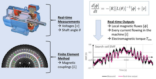
  • Any number of electrical circuits can be added to the models, including phase windings of course, but also bars, dampers and even search coils. This means the model can output actual currents flowing in bars and dampers and also local magnetic fluxes by using search coils.
  • It can compute distribution of power losses inside the machine [16], allowing calculations of local temperature elevation if used with a thermal model [17].
For these reasons, the CFE-CC model is very close to its physical counterpart. All it takes for building it is the FEM model, which is available from the design phase.
This work presents the methodology to implement for real-time execution the CFE-CC model fed with measurements taken from the real machine, thus allowing effective online monitoring of internal electromagnetic quantities. The proposed electromagnetic model can then be used alongside thermal and mechanical models to complement this real-time digital twin (RTDT). The machine used as case-study to realize the proposed RTDT is a wound rotor induction machine (WRIM), also known as doubly-fed induction machine. This particular type of machine was chosen because all of its electrical circuits are accessible for measurements, thus making it convenient for signal waveform validation. It is important to note however that the described method herein is applicable to every type of electrical machine. After a detailed explanation on the model’s construction and implementation on digital real-time simulator (DRTS), results are validated by comparing in real-time the RTDT’s outputs to the physical machine’s measurements.

2. CFE-CC Model Construction of a Wound Rotor Induction Machine

2.1. Model’s Equations

The model used for the purpose of this work does not include magnetic saturation. Iron losses as well as capacitive effects are also neglected.
A wound rotor induction machine, as well as many other types of electrical machines, comprises n electrical circuits where current can flow, such as the phases and bars. The total magnetic flux ϕ at a given circuit is the sum of the magnetic fluxes received from all other circuits and itself. It is worth noting that every quantity referenced in this manuscript is instantaneous and no referential transformation is used.
ϕ i = j = 1 n ϕ i j
The magnetic flux received at a given circuit from another one depends on the current i flowing in the sender and the magnetic coupling L between the two. The coupling is a function of the rotor angular position θ .
ϕ i j = L i j ( θ ) i j
All aforementioned equations are included into a single matrix equation:
[ ϕ ] = [ L ( θ ) ] [ i ]
Flux variation seen by any circuit creates a voltage v given by:
[ v ] = [ R ] [ i ] + d [ ϕ ] d t
By combining Equations (3) and (4), the dynamic system of Equation (5) is obtained.
d [ ϕ ] d t = [ R ] [ L ( θ ) ] 1 [ ϕ ] + [ v ]
As for electromagnetic torque T e m , it can be computed using:
T e m = 0.5 [ i ] T d [ L ( θ ) ] d θ [ i ]
For search coils or any electrical circuit always left open, Equation (7) is used instead to compute back-emf v w for better numerical stability of ordinary differential equations solvers. Matrix [ L w ] defines the coupling between the search coils and the other circuits carrying a current.
[ v w ] = d [ L w ] [ i ] d t
To sum up, identification of the model requires to know the inductance matrix function [ L ( θ ) ] which can then be inverted and differentiated. What makes the CFE-CC model versatile is the identification process of [ L ( θ ) ] with an FEM software. It uses a lookup table to store the inverse and derivative inductance matrix for many discrete positions of the rotor.
As in [14], it is possible to consider magnetic saturation with the precomputed inductance functions by using a correction coefficient afterward on computed magnetic flux linkages. Performances and computing time differ depending on type of machine and chosen quantities to compute the coefficient.

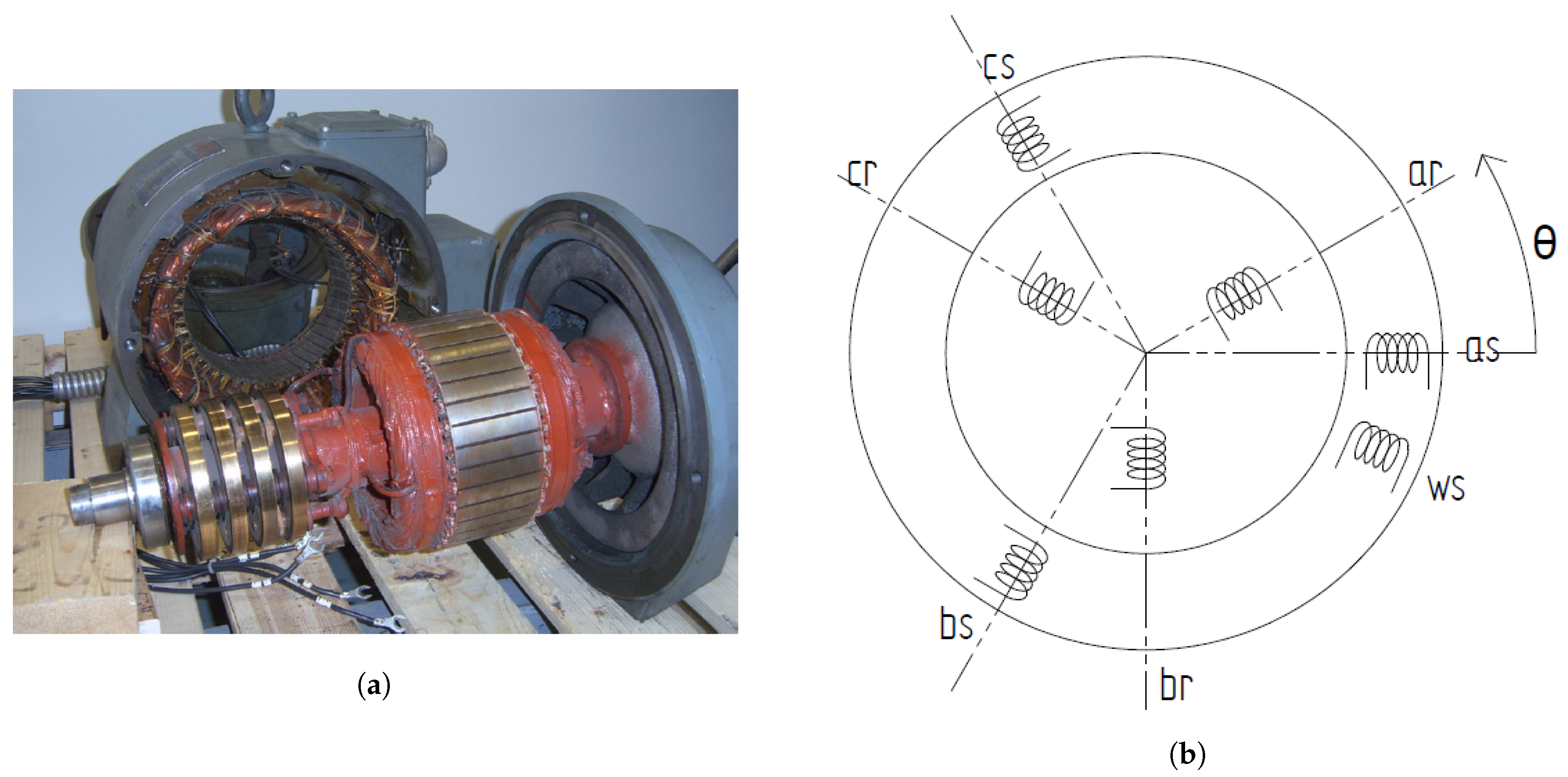
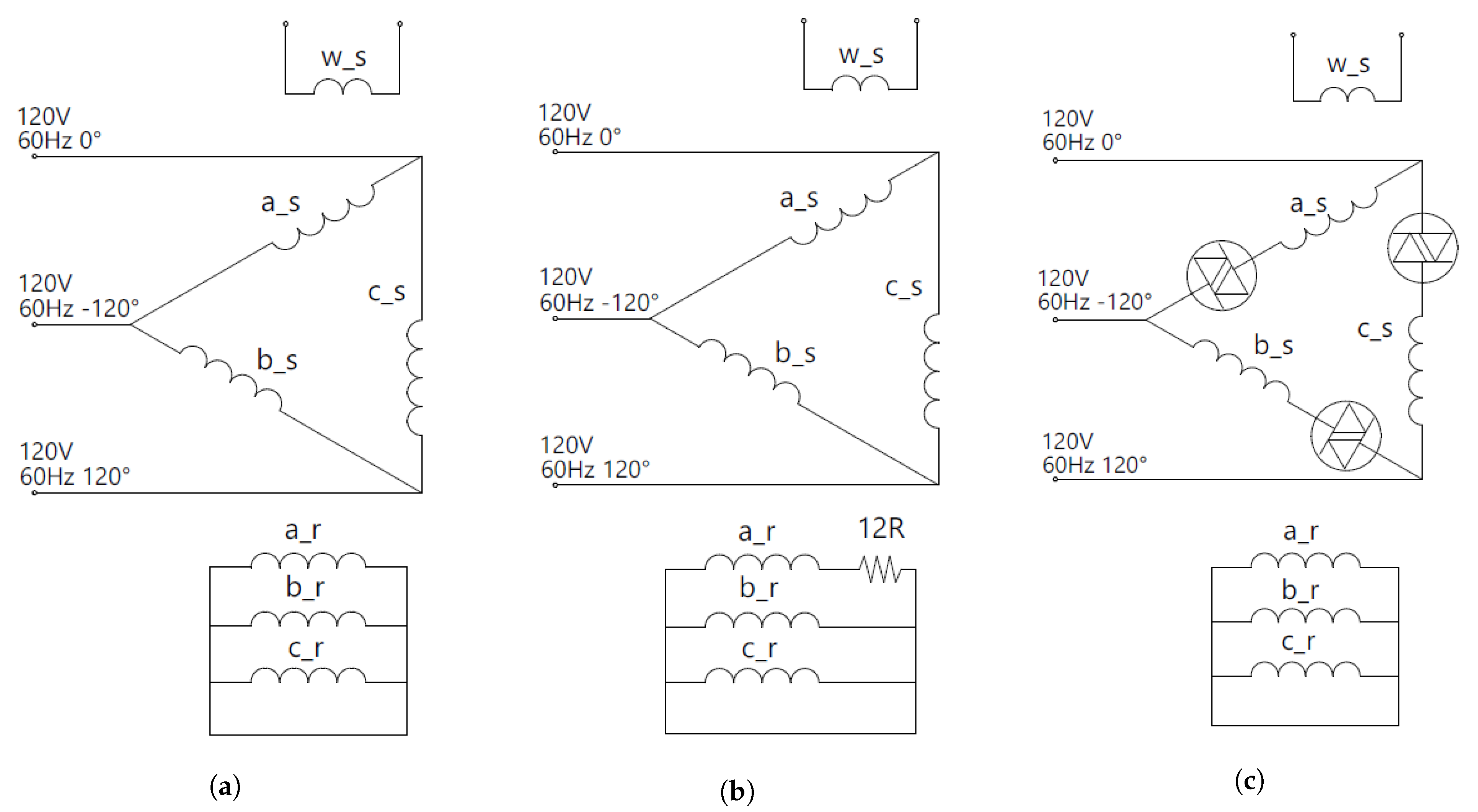
2.2. Identification of Electrical Circuits

Table 1 gathers specifications of the WRIM used in this work.
As depicted in Figure 1b, there are three windings on the stator ( a s , b s , c s ) and three windings on the rotor ( a r , b r , c r ). A small search coil is also added around one stator tooth ( w s ) in order to measure the voltage across it during operation. These seven circuits make up the CFE-CC model.
The resistance matrix [ R ] of the WRIM is diagonal as shown below. Each terminal is accessible so resistance values can easily be measured. The search coil is not included because it is left as an open circuit, thus Equation (7) is used instead of (5) for this particular case.
[ R ] = R a s 0 0 0 0 0 0 R b s 0 0 0 0 0 0 R c s 0 0 0 0 0 0 R a r 0 0 0 0 0 0 R b r 0 0 0 0 0 0 R c r
As for [ L ] , for any given rotor position, it has the form shown below. Magnetic couplings of the search coil are also included in a separate matrix [ L w ] .
[ L ] = L a s a s L a s b s L a s c s L a s a r L a s b r L a s c r L b s a s L b s b s L b s c s L b s a r L b s b r L b s c r L c s a s L c s b s L c s c s L c s a r L c s b r L c s c r L a r a s L a r b s L a r c s L a r a r L a r b r L a r c r L b r a s L b r b s L b r c s L b r a r L b r b r L b r c r L c r a s L c r b s L c r c s L c r a r L c r b r L c r c r
[ L w ] = L w s a s L w s b s L w s c s L w s a r L w s b r L w s c r

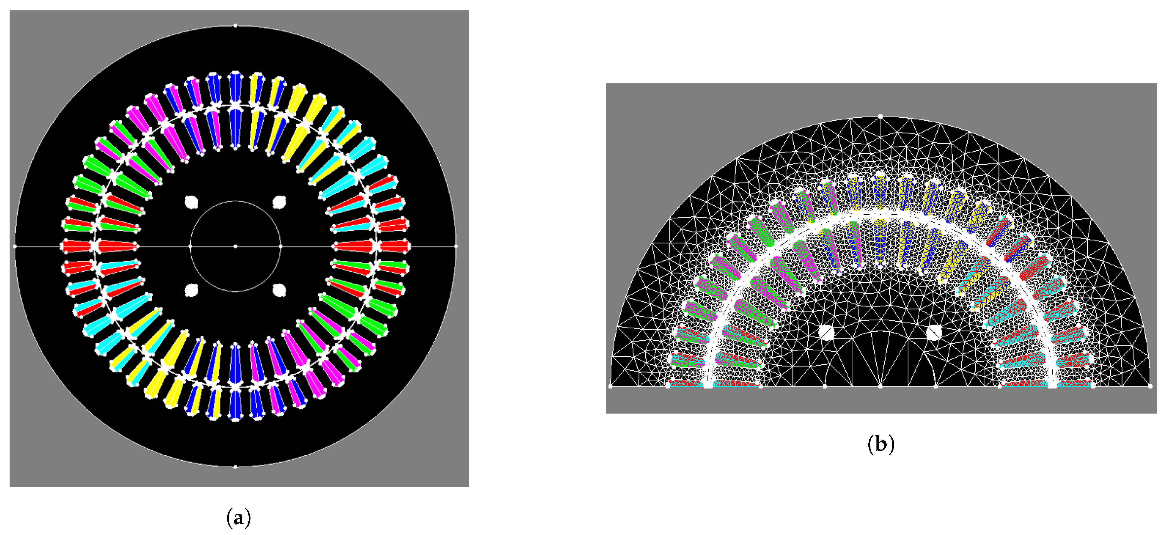
2.3. Computation of the Inductance Matrix Using FEM

Computation of [ L ( θ ) ] is performed with an FEM software and accurate plans of the machine geometry and windings. A 3D FEM software is an ideal choice as it consider geometries that are impossible to model in a 2D environment. However, a 2D FEM software is normally easier to use and less computationally expensive. It should be noted that computation time required to solve the finite element domain is not related to the CFE-CC model’s computation time at each time step, because results of the FEM are used as precomputed lookup tables.
For the present work, the authors opted for a 2D software to quickly compute [ L ( θ ) ] . The geometry of the WRIM makes it convenient to use a 2D space, but a few issues cannot be accounted in 2D alone such as rotor skewing and coil ends. Their respective effects are added to the model by altering the computed inductance matrix. Details of this procedure are presented at Appendix A. Figure 2 shows the FEM model of the WRIM in FLUX2D, the FEM software used for this work.
The domain can be reduced to only half of the complete machine because the machine has two pairs of poles and presents a symmetry. All magnetic materials are assumed to be linear, so saturation is not considered. Meshing is performed using the software’s automatic mesh tool. Mesh size was selected by comparing the solution obtained using a fine mesh to more and more coarse ones, until the error starts increasing noticeably. Once the FEM model is ready, the procedure for identifying magnetic couplings is launched. Inductance matrix [ L ] is computed for many rotor positions to build the lookup table.
Inductance matrix [ L ( θ ) ] is obtained by first computing the inductance matrix of the machine without windings, i.e., the inductance matrix of the slots [ L s l o t ( θ ) ] . That way, one may generate any winding configuration without restarting the FEM process simply by applying the following matrix transformation:
[ L ( θ ) ] = [ N ] T [ L s l o t ( θ ) ] [ N ]
[ N ] is the winding configuration matrix. It contains the number of turns N of each electrical circuit in each slot. Equation (12) shows how to build the matrix, where n c is the total number of circuits and n s is the total number of slot.
N = N 1 , 1 N 1 , 2 N 1 , n c N 2 , 1 N 2 , 2 N n s , 1 N n s , n c
In total, 1440 positions were computed evenly for a 180 rotation, i.e., 60 positions per stator slot pitch or an angular step of 0.125 . It is plenty to have a good resolution. Impact of inductance discretization is described thoroughly in [18]. At this point, it is important to take into consideration the physical memory to store the lookup table. Since the WRIM has six circuits without the search coil, the total number of elements in the lookup table for the inverse inductance matrix is 51,840. Another lookup table of the same size is necessary for the derivative if torque computation is included.

3. Hardware Setup

3.1. Real-Time Simulator And RT-Lab

The processing unit of the digital twin is an OP4510 entry-level DRTS of OPAL-RT. Real-time computations are performed by a dedicated multi-core CPU capable of time step of 2 μ s. For applications requiring smaller time step, one may rather opt for a higher-end DRTS or FPGA based platforms instead. Table 2 sums up the main technical specifications of the DRTS used in this work.
The OP4510 needs to be connected via an ethernet cable to a personal computer (PC) with RT-LAB installed. RT-LAB is a software environment for real-time simulation to interface with OPAL-RT’s DRTS. Using a PC and RT-LAB, user can:
  • Modify execution state of the program (run, stop, pause);
  • Change parameters in real-time of the running model;
  • Receive data from the running model.

3.2. Voltage and Current Measurement

Measured voltages are the inputs of the model. Currents are also measured, but they are used for validation purposes to compare with the RTDT’s outputs. A printed circuit board (PCB) was designed for voltage and current acquisition from the machine. The signals are then sampled using the DRTS’s analog input channels.

3.3. Angular Position Sensor
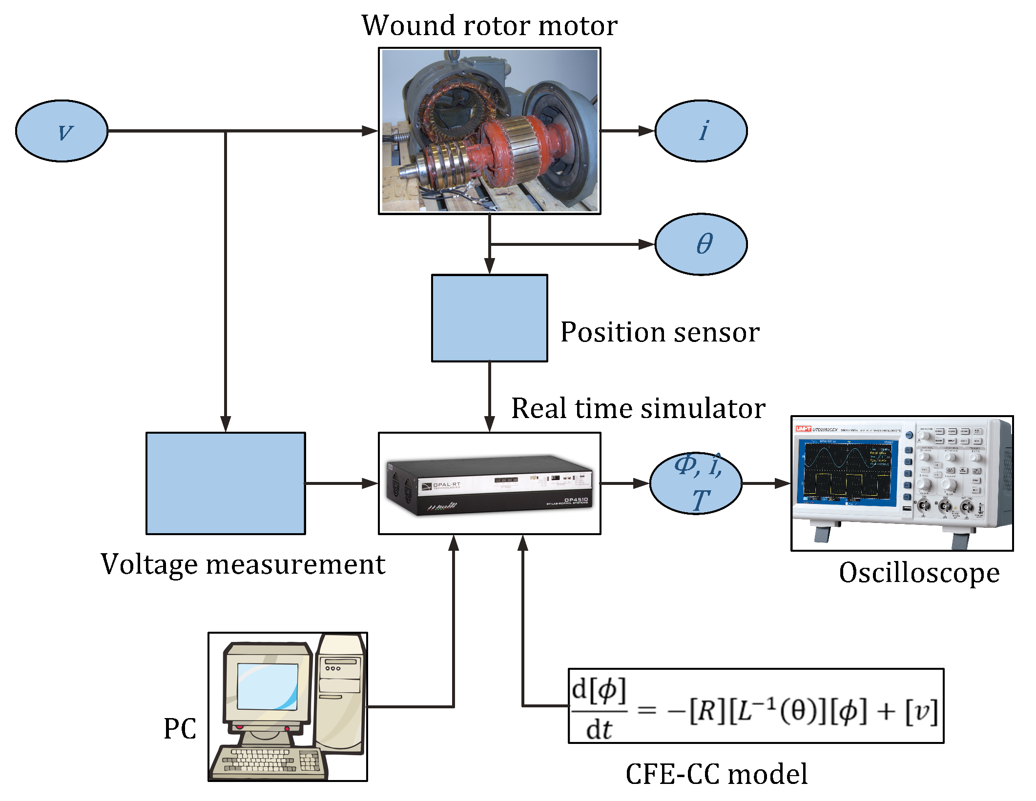
The angular position of the rotor is needed to retrieve the inductance matrix from the lookup table. It is measured using an absolute shaft encoder. The measured position is encoded in a 12 bits signal sent through a parallel communication interface. Each bit is acquired by a digital input channel of the DRTS and binary to decimal conversion is performed in software.

3.4. Setup Overview

Figure 3 shows an overview of the hardware setup. The CFE-CC model is executed in real-time along with the actual machine in operation. All estimated waveforms can be displayed on an oscilloscope using the DRTS’s analog output channels.

4. Implementation on Real-Time Simulator

4.1. Programming Method

Programming of the RTDT was realized entirely within the MATLAB/Simulink environment using RT-LAB. It generated C code from a Simulink block diagram and sent it to the DRTS for compilation and execution.

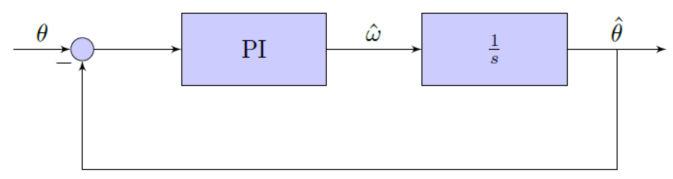
4.2. Position Tracking Scheme

The acquired position signal cannot be fed directly to the CFE-CC model after decimal conversion because it is a noisy discrete signal. The model would see speed impulsions that would impact its estimations. In order to filter the position signal, the control loop shown at Figure 4 was programmed in the DRTS.
The resulting closed loop transfer function is:
H ( s ) = θ ^ θ = K p s + K i s 2 + K p s + K i
where K p and K i are the PI controller’s proportional and integral gains. The measured position was transformed beforehand from a sawtooth waveform into a ramp. The difference between measured and estimated position was sent to a PI controller and an integrator. Hence, the error in steady state was theoretically reduced to zero. The controller’s gains should be chosen high enough to keep track of the speed variations of the machine.

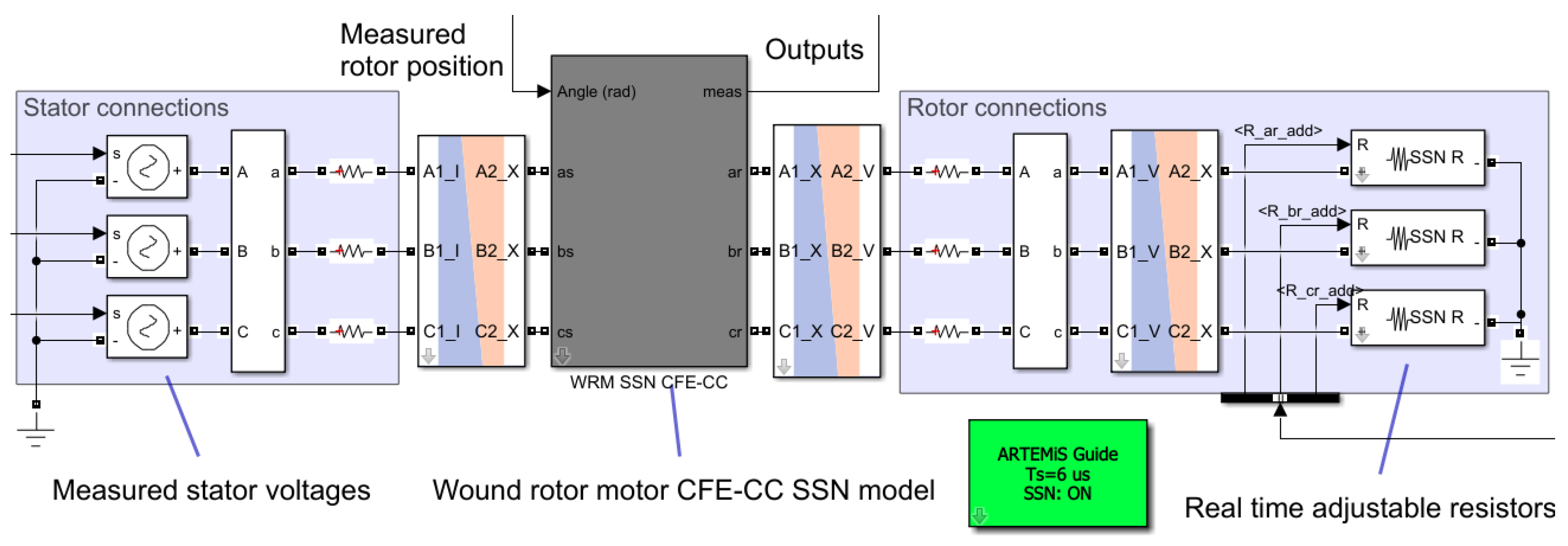
4.3. CFE-CC Model Implementation for Real-Time Execution

Resolution of the global system was achieved using the State-Space-Nodal (SSN) solver of OPAL-RT available in the ARTEMIS package [19]. It allowed us to solve power systems equations with a hybrid method between pure state-space and nodal approach [20]. It was built upon the SimPowerSystems (SPS) package, thus the Simulink diagram was designed the same way by using SPS blocks (resistances, sources, inductances, etc.).
A custom block made for SSN resolution was implemented for the CFE-CC model. Figure 5 shows the WRIM bloc containing the CFE-CC model’s equations as well as external components connected to it. The stator’s terminals were connected to controlled voltage sources, which were the measured stator voltages of the physical machine. The rotor’s terminals were connected to external resistors adjustable in real-time from the PC. By placing the machine in a separate nodal group than the external components, it had a decoupling effect with SSN resolution, thus greater stability was achieved even with large external resistances [21].
In order to implement such a model for SSN resolution, one must first select which circuits are available to the user as external connections, i.e., the Simulink block’s terminals of the machine. The WRIM had six circuits, all available for external connection, thus vectors [ v i n ] and [ i o u t ] were each six units large. They were respectively the input voltages and output currents at the Simulink block’s terminals. The search coil w s was not treated as a circuit because no current could flow through.
[ ϕ ] = ϕ a s ϕ b s ϕ c s ϕ a r ϕ b r ϕ c r T
[ v i n ] = v a s v b s v c s v a r v b r v c r T
[ i o u t ] = i a s i b s i c s i a r i b r i c r T
Dynamical system of Equation (5) is rearranged as standard state-space form. To facilitate reading of the following equations, the θ dependency is omitted.
[ ϕ ] = [ A ] [ ϕ ] + [ B ] [ v i n ]
[ i o u t ] = [ C ] [ ϕ ]
With
[ A ] = [ R ] [ L ] 1
[ B ] = [ I ]
[ C ] = [ L ] 1
Matrices [ B ] and [ C ] depend on the electrical terminals of the model. For the WRIM, [ B ] is equal to the identity matrix [ I ] since every circuit is also a terminal. For the same reason, matrix [ C ] is directly equal to [ L ] 1 .
SSN solver discretizes Equation (17) for a fixed time step T s using trapezoidal rule [21]:
[ ϕ ] k + 1 = [ A d ] [ ϕ ] k + [ B d ] [ v ] k + [ B d ] [ v ] k + 1
[ A d ] = ( [ I ] + [ A ] T s / 2 ) / ( [ I ] [ A ] T s / 2 )
[ B d ] = ( [ B ] T s / 2 ) / ( [ I ] [ A ] T s / 2 )
SSN solver needs the following two quantities from the CFE-CC model to operate:
[ Y C D M ] = [ C ] [ B d ]
[ i h i s t ] = [ C ] ( [ A d ] [ ϕ k ] + [ B d ] [ v k ] )
Matrices [ A d ( θ ) ] , [ B d ( θ ) ] and [ L ( θ ) ] 1 were stored in a lookup table. At each time step, the exact matrices were computed as the result of an interpolation between two adjacent matrices of the lookup table by using the angular position measurement. The same type of storage and interpolation was used to retrieve the derivative inductance matrix for torque computation using Equation (6).
Now regarding the search coil, since no current, i.e., no state, was associated with it, it was not included in the dynamical system. Instead, it was computed using Equation (7).

4.4. Time Step Selection
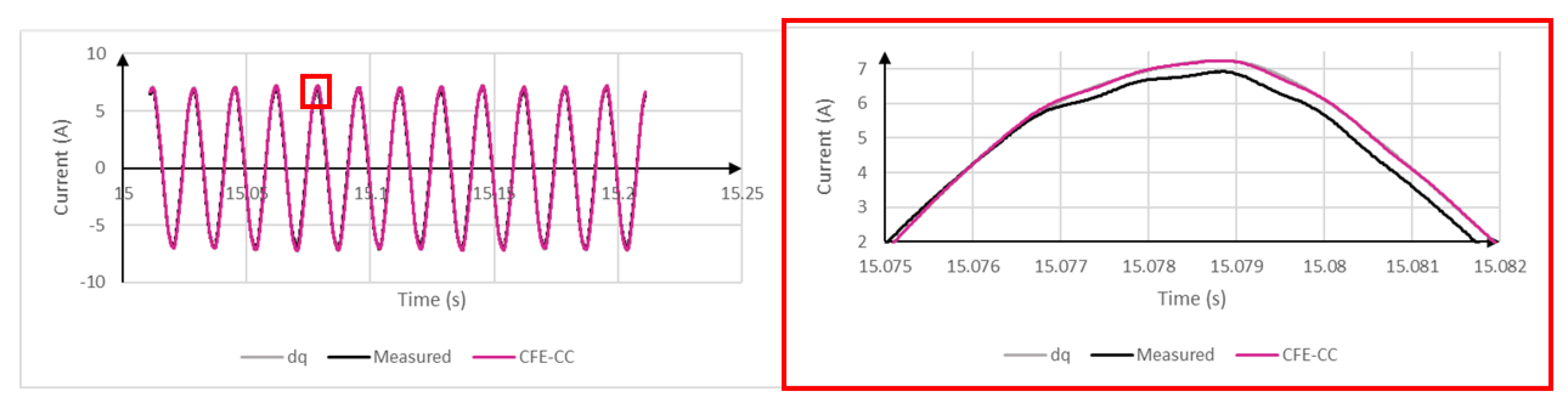
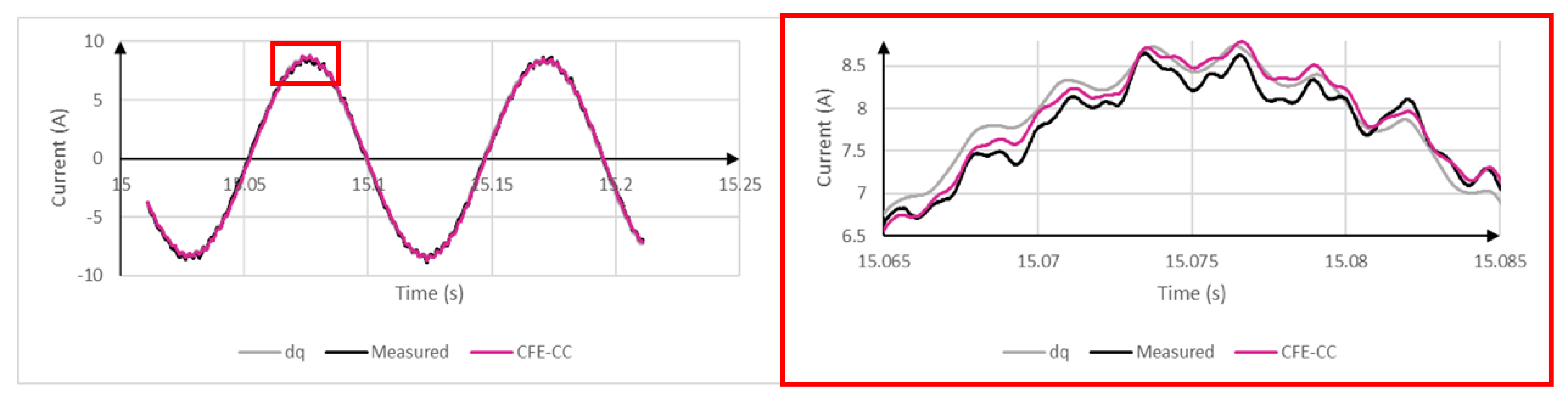
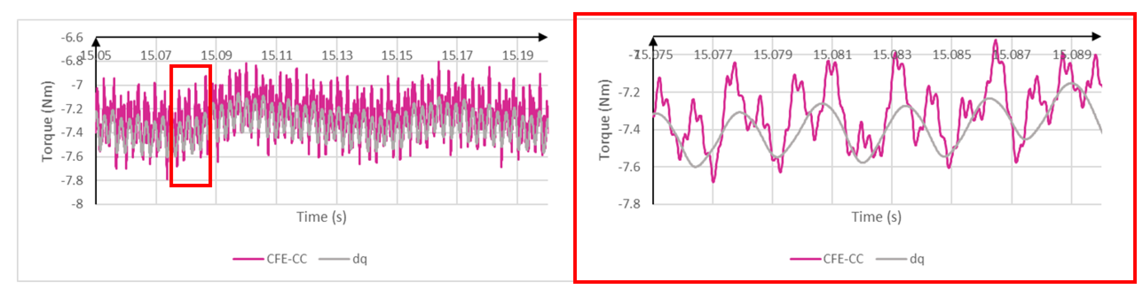
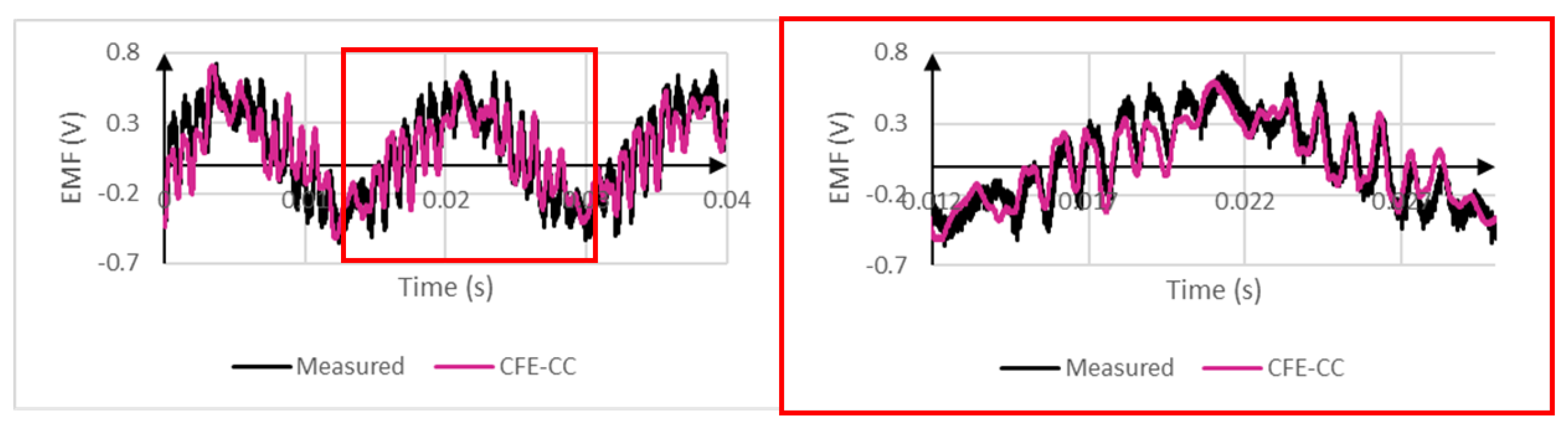
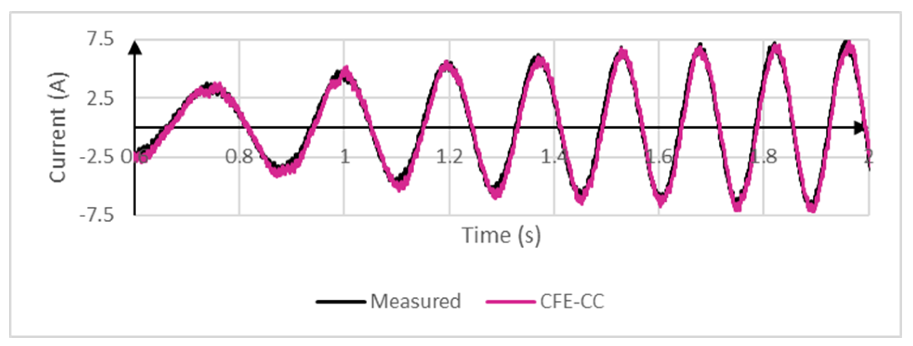
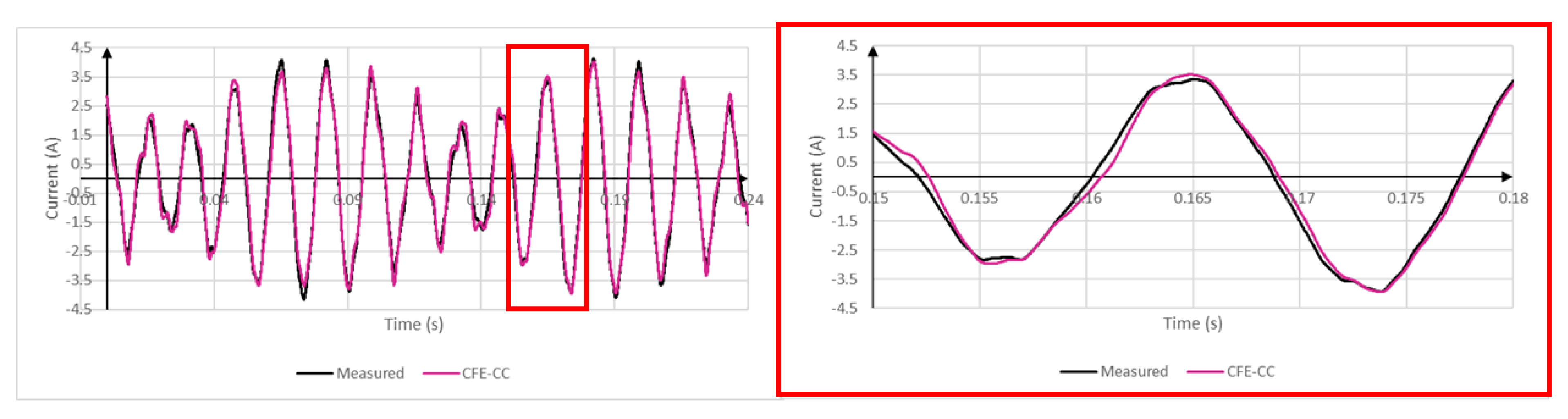
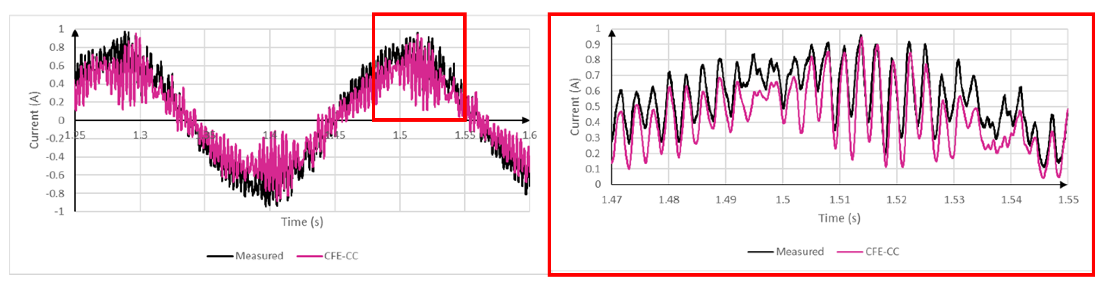
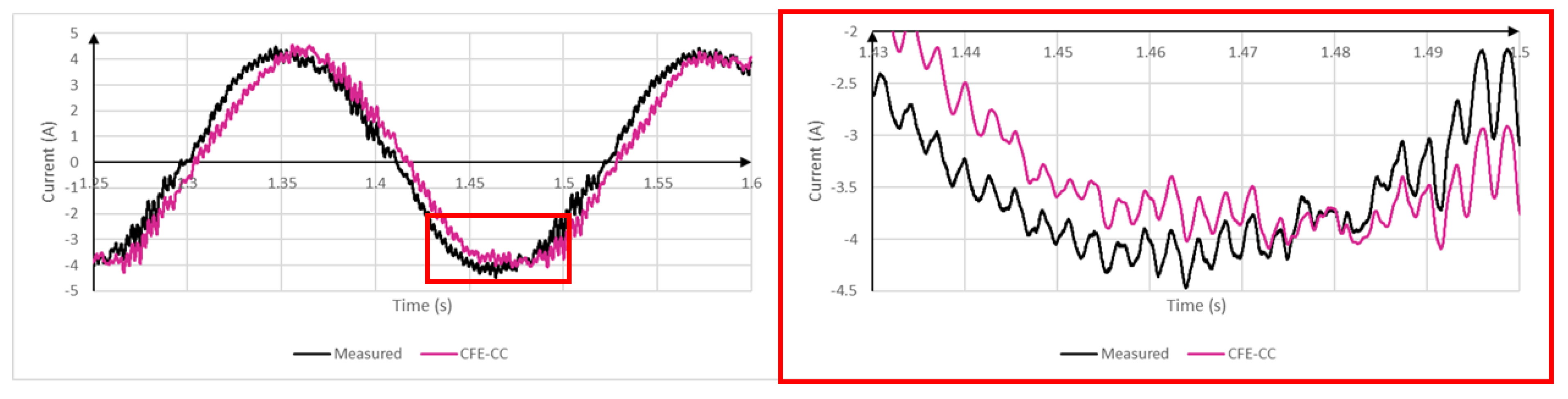
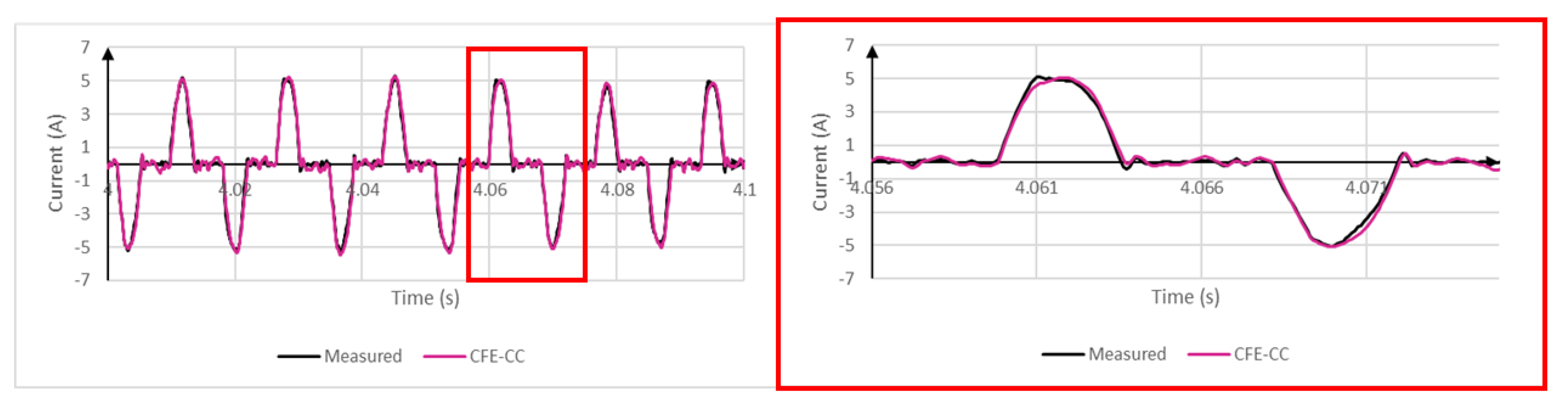
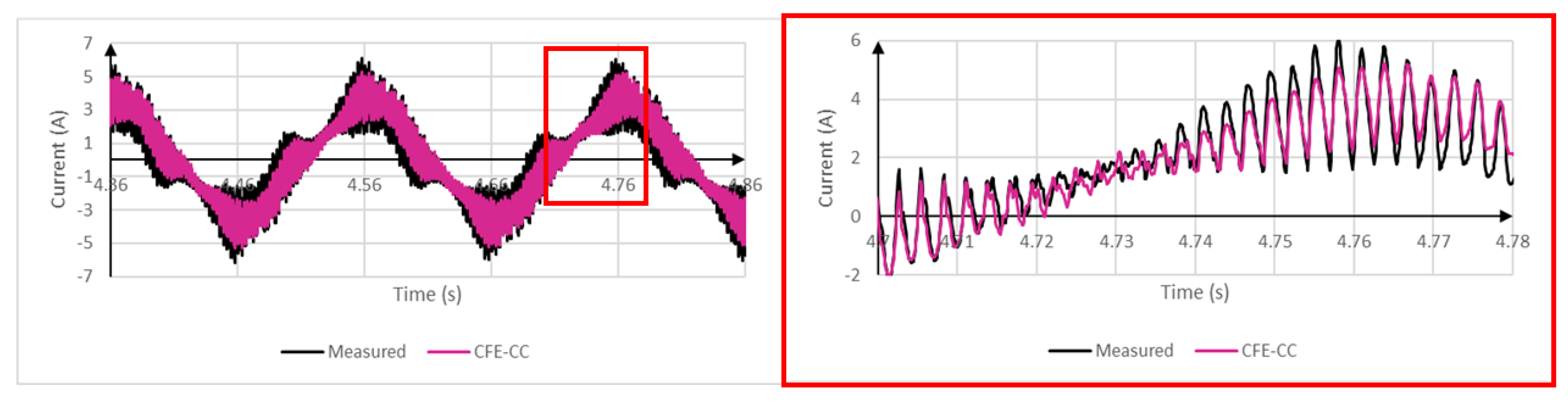
The execution time step of the program was chosen to be as small as possible without any risk of overrun. An overrun occurred if the DRTS did not finish all computations within the specified time step. In that case, a time step was skipped resulting in erroneous estimation. RT-LAB gives information regarding computational requirement of the program. Based on it, a time step of 6 μ s was chosen. It was important to have a small time step particularly when a circuit of the CFE-CC model was connected to a large external resistance. A large external resistance created a stiff state-space system, thus requiring a smaller time step to keep the solver stable. The SSN solver increased stability compared to the traditional approach but accuracy decreases when the time step was too large.

5. Validation

Validation of the RTDT was performed by comparing its real-time outputs to measurements available on the physical WRIM during operation. Waveforms shown below are real-time raw data acquired by an oscilloscope. For comparison purpose, a dq model of the WRIM was also implemented on another core of the DRTS for parallel execution alongside the CFE-CC model.
For the first setup, shown in Figure 6a, the WRIM’s stator windings were connected to a three-phase 60 Hz autotransformer. It was used as an induction motor, so rotor terminals were short-circuited. The WRIM was mechanically coupled to a synchronous generator loaded by resistors. Figure 7 and Figure 8 show waveform comparisons between measurements, CFE-CC model and dq model. Only winding a is shown because b and c were only 120 phase-shifted. Both models yielded good accuracy, but it was possible to draw more conclusions from the frequency decomposition. Table 3, Table 4 and Table 5 show the notables frequencies of the spectra. As expected, the CFE-CC model approximated well higher frequencies which were related to the geometry of the machine, whereas the dq model only computed harmonics related to input voltage.
Geometric irregularities of the machine had an impact on the torque as well, as seen from Figure 9. By analysing the electromagnetic torque of a machine, one can draw many conclusions about its condition.
Figure 10 shows the clear congruence between real-time output of the search coil voltage and its measured counterpart. Search coil voltage gave a good indication of local magnetic flux linkage. Using Equation (11), any number of search coils could be directly added to the machine’s winding configuration without restarting the FEM process. This also proved to be an interesting tool for online fault monitoring.
Figure 11 shows the dynamic response of rotor currents when the mechanical load was suddenly disconnected from the shaft. Here, the position tracking control loop played an important role. It needed to be fast enough to minimize the error during speed variations.
The following Figure 12, Figure 13 and Figure 14 show the RTDT’s current outputs when a phase imbalance was introduced. The setup is depicted at Figure 6b. A resistor was connected to winding a r of the physical machine, and the same was done to the RTDT. While the frequency content was accurate, a small phase discrepancy was present at winding b r and c r . The cause could be related to the methodology employed to compute [ L ] in Appendix A, such as the way the coil end inductances were added. Many assumptions were made. Magnetic saturation could also play a role since it was not taken into account in the model.
Finally, TRIACs were added inside the delta configuration as depicted in Figure 6c. It demonstrated the RTDT’s behavior under switching converter’s voltage input for an unusual phase configuration. Figure 15 and Figure 16 show currents flowing in windings a s and a r . The RTDT yielded accurate estimations.

6. Conclusions

The detailed CFE-CC model of a WRIM was implemented in real-time on an entry-level DRTS of OPAL-RT with a time step of 6 μ s. This model considers the machine’s particular geometry and winding configuration can be changed easily using a simple matrix transformation. Any number of search coils can be added to the model, as well as faults such as broken bar and eccentricity. Comparisons with real-time measurements have shown that the CFE-CC model is accurate and computationally efficient. This work paves the way to new real-time monitoring techniques for electrical machines using the CFE-CC model alongside others in a digital twin. However, the machine studied in this work has only seven circuits. Including more electrical circuits in the CFE-CC model results in more computations at each time step and more memory requirement for lookup tables. Future works include studying the feasibility of real-time execution of the CFE-CC model for large synchronous machines comprising many electrical circuits.

Author Contributions

Conceptualization, S.B.; methodology, S.B.; software, S.B.; validation, S.B.; formal analysis, S.B., P.V. and J.C.; investigation, S.B.; resources, S.B.; data curation, S.B.; writing—original draft preparation, S.B.; writing—review and editing, S.B., P.V. and J.C.; supervision, P.V.; project administration, P.V. and J.C.; funding acquisition, P.V. and J.C. All authors have read and agreed to the published version of the manuscript.

Funding

This research received no external funding.

Acknowledgments

The authors would like to thank OPAL-RT for their support in this work.

Conflicts of Interest

The authors declare no conflict of interest.

Abbreviations

The following abbreviations are used in this manuscript:
WRIMWound rotor induction machine
DRTSDigital real-time simulator
RTDTReal-time digital twin
CFE-CCCombination of finite element and coupled circuits
FEMFinite element method
SSNState-Space-Nodal
SPSSimPowerSystems

Appendix A. Alteration of Inductance Matrix to Consider Rotor Skew and Coil Ends

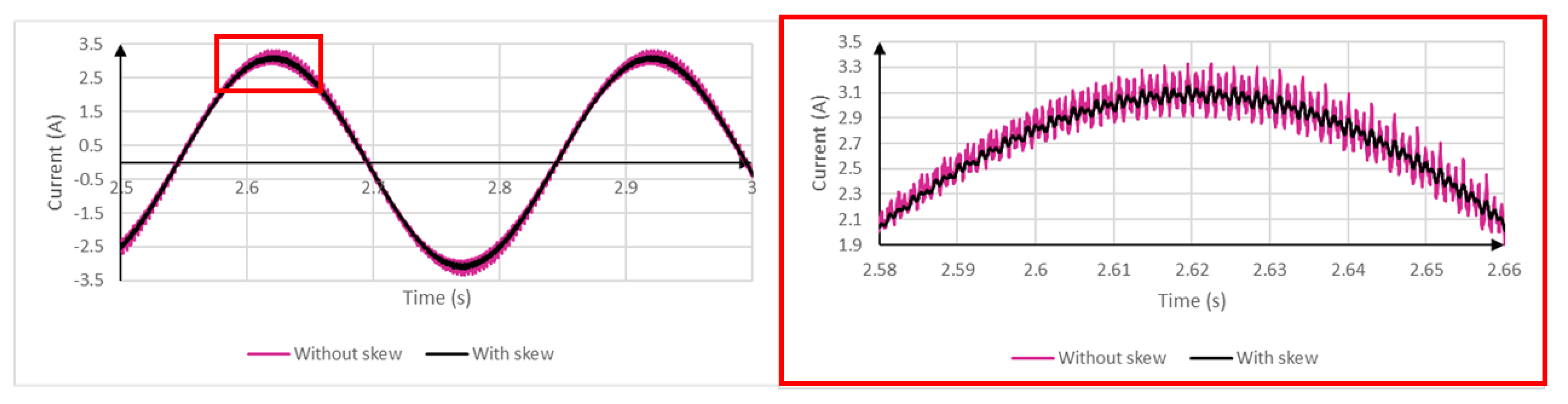
Appendix A.1. Rotor Skewing

The 2D FEM software used in this work suppose a uniform magnetic field intensity along the third dimension. However, the WRIM and most asynchronous machines have a skewed rotor to prevent cogging and reduce torque oscillations. The skew angle θ s k is generally given by the manufacturer. Fortunately, it is possible to add this effect into the inductance matrix [ L ( θ ) ] previously identified in 2D [22]. By dividing an unskewed machine along its length into M several slices, or sub-machines, the inductance matrix [ L m ( θ ) ] of each sub-machine is simply the initial one [ L ( θ ) ] divided by M.
[ L ( θ ) ] = [ L 1 ( θ ) ] + [ L 2 ( θ ) ] + [ L M ( θ ) ]
[ L m ( θ ) ] = [ L ( θ ) ] / M , m = 1 , 2 , M
Now, it is possible to replicate the skewing effect by shifting the rotor gradually along the length. Each of the inductance matrices [ L 1 ( θ ) ] [ L M ( θ ) ] needs to be shifted by θ s k / ( M 1 ) . Finally, they can be added all together according to Equation (A1) to obtain the skewed [ L ( θ ) ] of the complete machine.
As for the WRIM of this work, θ s k is equal to 7.5 , which corresponds to a slot pitch. The machine was divided into 61 sub-machines. Figure A1 shows the impact of the added skew effect on rotor currents during load operation, with stator windings fed with perfectly sinusoidal voltages and rotor windings short-circuited. Current ripples are reduced as expected.
Figure A1. Rotor current with and without added rotor skewing effect, enlarged on right side.
Energies 13 05413 g0a1

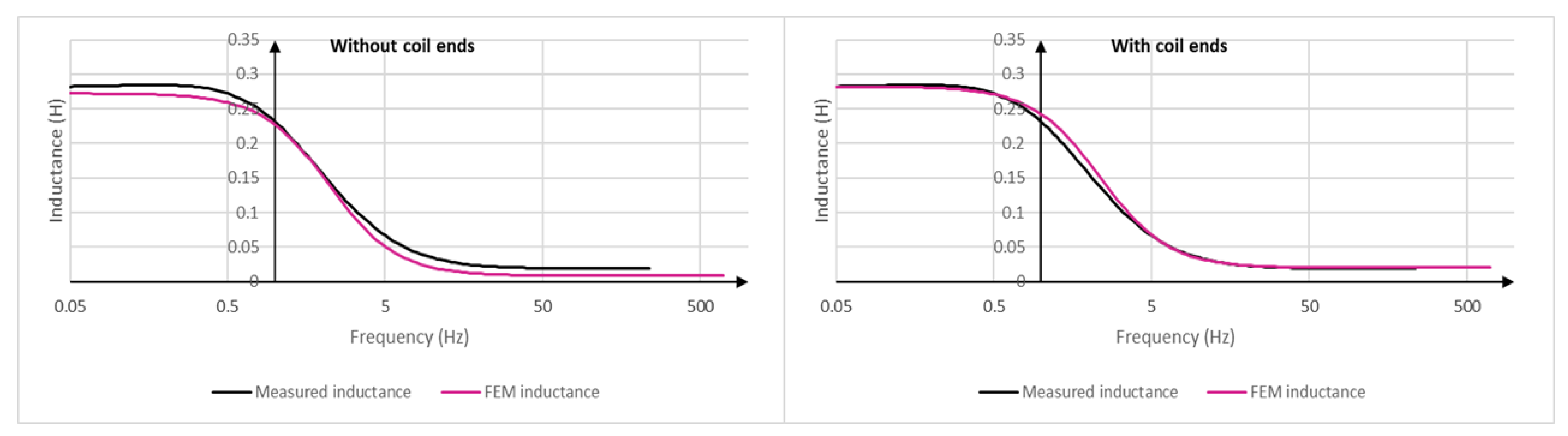
Appendix A.2. Coil Ends

Coil ends can be modeled in a 3D FEM software, whereas it cannot be in 2D. In the latter case such as in the present work, their inductive effect must be added to [ L ( θ ) ] by other means. For simplicity, we ignore the impact on mutual inductances. The technique used is to conduct a standstill frequency response (SSFR) test [14] and add a self-inductance to the windings in order to make the experimental response fit the simulated one. The test was conducted while rotor windings are short-circuited. Figure A2 compares the response of the FEM model to the experiment with and without coil ends. Inductances of 0.01 H and 0.00047 H were added to stator and rotor windings respectively, which is less than 10% of the magnetizing inductance.
Figure A2. Inductance seen from the stator versus frequency with and without coil ends, rotor terminals short-circuited.
Energies 13 05413 g0a2

References

  1. Ebrahimi, A. Challenges of developing a digital twin model of renewable energy generators. In Proceedings of the 2019 IEEE 28th International Symposium on Industrial Electronics (ISIE), Vancouver, BC, Canada, 12–14 June 2019; pp. 1059–1066. [Google Scholar]
  2. Wang, J.; Ye, L.; Gao, R.X.; Li, C.; Zhang, L. Digital Twin for rotating machinery fault diagnosis in smart manufacturing. Int. J. Prod. Res. 2019, 57, 3920–3934. [Google Scholar] [CrossRef]
  3. Boschert, S.; Heinrich, C.; Rosen, R. Next generation digital Twin. In Proceedings of the TMCE, Las Palmas de Gran Canaria, Spain, 7–11 May 2018. [Google Scholar]
  4. Fuller, A.; Fan, Z.; Day, C.; Barlow, C. Digital Twin: Enabling Technologies, Challenges and Open Research. IEEE Access 2020, 8, 108952–108971. [Google Scholar] [CrossRef]
  5. Roshandel Tavana, N.; Dinavahi, V. A General Framework for FPGA-Based Real-Time Emulation of Electrical Machines for HIL Applications. IEEE Trans. Ind. Electron. 2015, 62, 2041–2053. [Google Scholar] [CrossRef]
  6. Kłosowski, Z.; Cieślik, S. Real-time simulation of power conversion in doubly fed induction machine. Energies 2020, 13, 673. [Google Scholar] [CrossRef] [Green Version]
  7. Sidwall, K.; Forsyth, P. Advancements in Real-Time Simulation for the Validation of Grid Modernization Technologies. Energies 2020, 13, 4036. [Google Scholar] [CrossRef]
  8. Mojlish, S.; Erdogan, N.; Levine, D.; Davoudi, A. Review of Hardware Platforms for Real-Time Simulation of Electric Machines. IEEE Trans. Transp. Electrif. 2017, 3, 130–146. [Google Scholar] [CrossRef]
  9. Sudhoff, S.D.; Kuhn, B.T.; Corzine, K.A.; Branecky, B.T. Magnetic Equivalent Circuit Modeling of Induction Motors. IEEE Trans. Energy Convers. 2007, 22, 259–270. [Google Scholar] [CrossRef]
  10. Fleming, F.E.; Edrington, C.S. Real-Time Emulation of Switched Reluctance Machines via Magnetic Equivalent Circuits. IEEE Trans. Ind. Electron. 2016, 63, 3366–3376. [Google Scholar] [CrossRef]
  11. Jandaghi, B.; Dinavahi, V. Real-Time HIL Emulation of Faulted Electric Machines Based on Nonlinear MEC Model. IEEE Trans. Energy Convers. 2019, 34, 1190–1199. [Google Scholar] [CrossRef]
  12. Luo, X.; Liao, Y.; Toliyat, H.; El-Antably, A.; Lipo, T.A. Multiple Coupled Circuit Modeling of Induction Machines. In Proceedings of the Conference Record of the 1993 IEEE Industry Applications Conference Twenty-Eighth IAS Annual Meeting, Toronto, ON, Canada, 2–8 October 1993; pp. 203–210. [Google Scholar] [CrossRef]
  13. Dehkordi, A.B.; Neti, P.; Gole, A.; Maguire, T. Development and validation of a comprehensive synchronous machine model for a real-time environment. IEEE Trans. Energy Convers. 2009, 25, 34–48. [Google Scholar] [CrossRef]
  14. Gbégbé, A.Z.; Rouached, B.; Cros, J.; Bergeron, M.; Viarouge, P. Damper Currents Simulation of Large Hydro-Generator Using the Combination of FEM and Coupled Circuits Models. IEEE Trans. Energy Convers. 2017, 32, 1273–1283. [Google Scholar] [CrossRef]
  15. Quéval, L.; Ohsaki, H. Study on the implementation of the phase-domain model for rotating electrical machines. In Proceedings of the 2012 15th International Conference on Electrical Machines and Systems (ICEMS), Sapporo, Japan, 21–24 October 2012; pp. 1–6. [Google Scholar]
  16. Rouached, B.; Cros, J.; Clénet, S.; Viarouge, P. Estimation of Damper Bars Losses in Large Synchronous Alternator using Bar Current Waveforms; Electrimacs: Toulouse, France, 2017. [Google Scholar]
  17. Demetriades, G.D.; de la Parra, H.Z.; Andersson, E.; Olsson, H. A Real-Time Thermal Model of a Permanent-Magnet Synchronous Motor. IEEE Trans. Power Electron. 2010, 25, 463–474. [Google Scholar] [CrossRef]
  18. Mathault, J.; Bergeron, M.; Rakotovololona, S.; Cros, J.; Viarouge, P. Influence of Discrete Inductance Curves on the Simulation of a Round Rotor Generator Using Coupled Circuit Method; Electrimacs: Valencia, Spain, 2014. [Google Scholar]
  19. Dufour, C.; Mahseredjian, J.; Belanger, J. A Combined State-Space Nodal Method for the Simulation of Power System Transients. IEEE Trans. Power Deliv. 2011, 26, 928–935. [Google Scholar] [CrossRef]
  20. Wang, L.; Jatskevich, J.; Dinavahi, V.; Dommel, H.W.; Martinez, J.A.; Strunz, K.; Rioual, M.; Chang, G.W.; Iravani, R. Methods of Interfacing Rotating Machine Models in Transient Simulation Programs. IEEE Trans. Power Deliv. 2010, 25, 891–903. [Google Scholar] [CrossRef]
  21. Dufour, C.; Nasrallah, D.S. State-space-nodal rotating machine models with improved numerical stability. In Proceedings of the IECON 2016—42nd Annual Conference of the IEEE Industrial Electronics Society, Florence, Italy, 23–26 October 2016; pp. 4368–4375. [Google Scholar] [CrossRef]
  22. Mohr, M.; Bíró, O.; Stermecki, A.; Diwoky, F. A Finite Element-Based Circuit Model Approach for Skewed Electrical Machines. IEEE Trans. Magn. 2014, 50, 837–840. [Google Scholar] [CrossRef]
Figure 1. (a) Photo of the wound rotor induction machine (WRIM) showing its stator and rotor; (b) circuits of the WRIM used to build the model.
Energies 13 05413 g001
Figure 2. (a) WRIM rendered in FLUX2D (b) Meshed domain.
Energies 13 05413 g002
Figure 3. Hardware setup overview.
Energies 13 05413 g003
Figure 4. Control loop to filter out position sensor’s noise.
Energies 13 05413 g004
Figure 5. Real-time digital twin (RTDT) implementation overview in Simulink using ARTEMIS package.
Energies 13 05413 g005
Figure 6. WRIM setups used for validation. (a) Balanced; (b) With rotor unbalance; (c) With TRIACs.
Energies 13 05413 g006
Figure 7. Stator current in winding a s during load operation, enlarged on right side.
Energies 13 05413 g007
Figure 8. Rotor current in winding a r during load operation, enlarged on right side.
Energies 13 05413 g008
Figure 9. Electromagnetic torque during load operation, enlarged on right side.
Energies 13 05413 g009
Figure 10. Search coil voltage during load operation, enlarged on right side.
Energies 13 05413 g010
Figure 11. Rotor current in winding a r starting from load operation and suddenly disconnecting the load.
Energies 13 05413 g011
Figure 12. Stator current in winding a s during load operation with 12 ohm resistor on winding a r , enlarged on right side.
Energies 13 05413 g012
Figure 13. Rotor current in winding a r during load operation with 12 ohm resistor on winding a r , enlarged on right side.
Energies 13 05413 g013
Figure 14. Rotor current in winding b r during load operation with 12 ohm resistor on winding a r , enlarged on right side.
Energies 13 05413 g014
Figure 15. Stator current in winding a s during load operation and fed through TRIACs, enlarged on right side.
Energies 13 05413 g015
Figure 16. Rotor current in winding a r during load operation and fed through TRIACs, enlarged on right side.
Energies 13 05413 g016
Table 1. Specifications of the WRIM.
ParameterValueUnit
Power rating1864W
Rated voltage208V
Number of phases3
Number of poles4
Number of stator slots48
Number of rotor slots36
Frequency60Hz
Speed1690RPM
Power factor0.81
Table 2. Technical specifications of the OP4510 real-time digital simulator.
CPUIntel Xeon E3 v5 CPU (4 core, 8 MB cache, 2.1 or 3.5 GHz)
Dynamic memory16 GB RAM
Storage128 GB SSD
Digital outputs32 channels, 5 V to 30 V adjustable by a user-supplied voltage
Digital inputs32 channels, 4 V to 50 V
Analog inputs16 channels, 16 bits, ±20 V true differential
Analog outputs16 channels, 16 bits, ±16 V
Table 3. Main frequency components of stator input voltage.
Frequency (Hz)Measurements (V)
60156.5
1801.0
3003.9
4201.8
Table 4. Main frequency components in stator current.
Frequency (Hz)Measurements (A)CFE-CC (A)dq (A)
605.7805.8655.916
1800.0500.0680.102
3000.1190.1020.102
4200.0510.0510.051
5880.0100.010n/a
9130.0150.013n/a
10330.0170.015n/a
Table 5. Main frequency components in rotor current.
Frequency (Hz)Measurements (A)CFE-CC (A)dq (A)
6.47.1307.2867.384
1140.1830.1160.117
3540.1390.1250.129
3670.0550.0440.045
6420.0140.013n/a
6550.0140.015n/a
9670.0180.015n/a
9790.0230.021n/a
Publisher’s Note: MDPI stays neutral with regard to jurisdictional claims in published maps and institutional affiliations.

