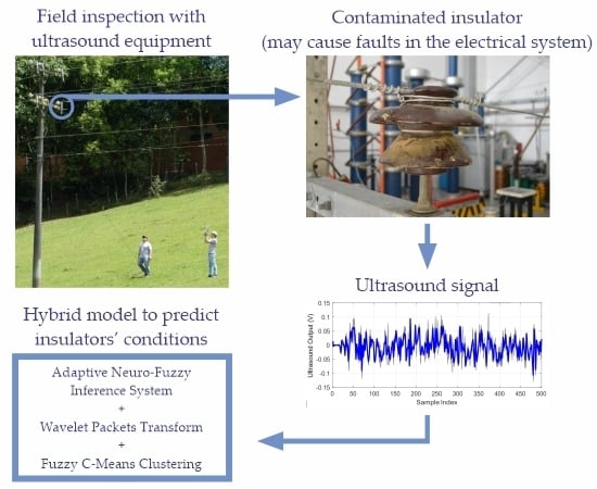
1. Introduction
Power grid insulators are responsible for supporting cables and keeping the system isolated from the ground and the other voltage phases. As these insulators are exposed to the environment, they may get contaminated by small particle deposits on their surface. The contamination does not necessarily mean that the insulator needs to be replaced, but if this contamination remains or increases, it may lead to a system failure [
1]. In practice, the protection switchgear (recloser) would disconnect the line. If the insulator was seriously damaged and the defect was permanent, field personnel would have to be sent to replace the insulator; otherwise, the recloser will put the line back in service and it will work as mentioned before.
As presented in [
2], fault location and identification associated with the electrical system is considered an important issue in order to ensure the efficiency of the services associated with energy distribution. For the inspection of the electrical system and faulty insulators location, ultrasound detectors are used, which capture the ultrasonic noise of the network components. The signal generated by this equipment is an audio signal, which is electronically sampled in a time series form [
3]. In order to predict the continuity of the signal generated by the ultrasound detector, an evaluation based on a modified version of the Wavelet Neuro-Fuzzy is presented in this article.
An Adaptive Neuro-Fuzzy Inference System (ANFIS) is a particular type of Artificial Neural Network (ANN) based on the Takagi–Sugeno–Kang inference model. The ANFIS method couples the benefits of both feedforward ANNs and fuzzy system techniques in the same framework [
4]. Considering the best characteristics of each technique, the neuro-fuzzy network can be used to handle systems that involve inaccurate, complex and nonlinear data [
5].
Neuro-fuzzy systems inherit learning and classification capacity, robustness, adaptation, nonlinear mapping, and clustering characteristics from ANNs. The behavior of these models can be understood through the observation of variables associated with the membership functions, the relationship between inputs and outputs, and from fuzzy rules due to similarities to human languages. From these aspects, the ANFIS method could be adopted for chaotic time series forecasting [
6,
7,
8,
9].
The idea of using ANFIS in this study was based on the success of applications of hybrid models. Actually, many techniques are available for the purpose of prediction, but hybrid techniques present consistent results when applied to both classification and time series forecasting applications [
10,
11]. In [
10], assuming public datasets with concept drift, the authors proposed an ensemble technique based on the Random Forest algorithm. The algorithm exploits ensemble pruning as a forgetting strategy, and the results performed better in classification when compared to other state-of-the-art concept drift classifiers. Additionally, in [
11], both wind speed and power were assumed as case studies to propose a hybrid strategy, named the ultra-short-time forecasting method, based on the Takagi–Sugeno fuzzy model. The antecedent and the consequent parts of the inference system were identified by the fuzzy c-means clustering algorithm, which was associated with the recursive least squares method. Considering wind farms from both China and Ireland, the proposed approach was compared with Support Vector Machines (SVM), empirical mode decomposition, and a classical back-propagation neural network, where the proposed method was shown to better predict short-term wind power.
In this article, the ANFIS model was employed for time series forecasting with the objective of evaluating its performance in predicting electrical insulator conditions, those available in the distribution network and which are susceptible to different climate and environment conditions. In this study, the signal adopted as an input for the model came from ultrasonic equipment used for electrical network inspection. Considering a normalized time series, feature extraction was performed by Wavelet Packets Transform (WPT) [
9], which allows signal simplification in both time and frequency domains considering its entropy, energy, and variation.
By associating wavelets and ANNs based on a fuzzy system, recent research has shown promising results in distinct applications. In the work presented in [
12], a novel fuzzy neural network structure assuming a cerebellar model neural network (CMNN) was proposed. Combining the advantages of wavelets associated with CMNN and the Takagi–Sugeno–Kang inference model, the authors compared the proposed method with traditional ANN structures, showing promising results for uncertain nonlinear systems identification.
In [
13], a hybrid fuzzy wavelet neural network (HFWNN) was proposed, and the algorithm parameters were initialized considering the fuzzy c-means clustering method (FCM). The proposed approach considered the first layer of the network to reflect data uncertainties, while a flexible second layer performed linear combinations of the wavelet function. In this case, the HFWNN parameters were adjusted assuming a genetic algorithm optimization procedure.
Another application involving both fuzzy and wavelet methods was presented in [
14], where a polynomial neural network, also assuming FCM, was applied in the premise operator to overcome dimensionality problems, while the consequence part was determined by means of wavelet functions whose parameters were estimated with the aid of the least squares method. The proposed algorithm showed an impressive ability to describe nonlinear relations between input and output variables, especially in regression and system identification problems.
Based on features extraction, an approach considering the ANFIS method associated with both wavelet and Fourier transforms was presented in [
15] to solve a classification task, with the main purpose of identifying the electrical energy quality provided to an electrical system. Similar works assuming ANFIS to deal with identification or classification of electrical systems failures were presented in [
16,
17].
A comparison between the fuzzy learning vector quantization used in clustering, Levenberg–Marquardt, and ANFIS based on input signals provided from the wavelet transform was presented in [
18]. Considering a classification case study, the objective was to evaluate fundus eye images in order to identify retinal abdominal eye disease. In this case, all methods presented 100% of success in solving this task.
An application concerning electrical energy price prediction based on both wavelets and ANFIS was presented in [
19]. Following the same line as previous works mentioned in this article, the technique provided consistent results in terms of prediction even considering the nonlinear characteristic of the data set. A study assuming three performance indices to compare ANFIS with both classical ANN structure and Multivariate Linear Regression (MLR) models was presented in [
20]. The main idea was to solve the prediction problem associated with the wastewater quality of the Las Vegas Wash, which is a 12-mile-long channel that feeds most of the Las Vegas Valley. The authors showed that ANFIS provided better results in terms of prediction when compared to classical ANN and MLR techniques.
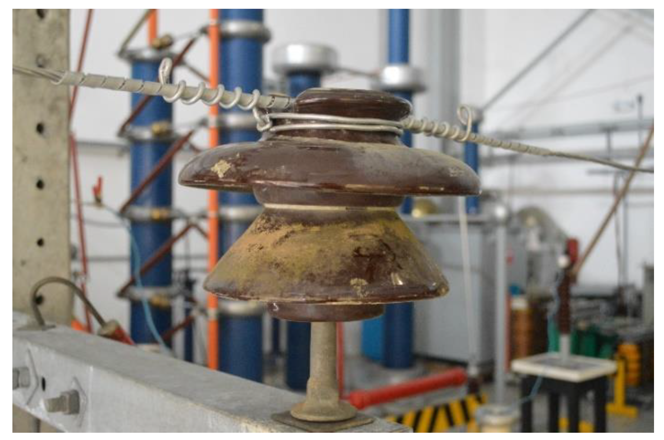
Taking into account the necessity of predictive maintenance to avoid electrical system failures, those associated with electrical insulator conditions, and the consistent results provided by the ANFIS method in time series forecasting applications presented above, this research proposes the use of Wavelet Packets Transform for both signal preprocessing and feature extraction based on a data set obtained from ultrasonic equipment considering a laboratory experiment in which a contaminated electrical insulator removed from an actual transmission line was assumed for data acquisition.
As mentioned before, contaminated insulators could be the reason for electrical system failures. To avoid this situation, the prediction of the insulator condition assuming a modified ANFIS method was performed in this study considering three approaches: (i) grid partition [
21]; (ii) subtractive clustering [
22]; and (iii) fuzzy c-means clustering [
23]. This paper presents a complete statistical evaluation of the capabilities of the ANFIS algorithm combined with WPT to predict the development of a fault in insulators of the electrical distribution system based on time series forecasting procedures.
The next section of this paper describes the problem related to the contamination of electrical insulators and their proper classification.
Section 3 presents experimental procedures for data acquisition, and
Section 4 addresses the proposed method assumed for time series forecasting.
Section 5 shows the results and discusses the method performance. Finally,
Section 6 reports the conclusions and future works associated with this research.
2. Description of the Electrical Insulator Problem
For more than a century, porcelain insulators have been used to support and insulate aerial conductors on transmission and distribution systems. Despite recent polymeric insulators being lighter, ceramic insulators are still being used, and some utilities still prefer them over the polymeric ones [
24]. Since transmission and distribution systems run over wide and open areas, the insulators used in these systems are subjected to environmental stresses, such as pollution and contamination, along with the normally applied voltage and mechanical loads. Transient voltage due to lightning or transient mechanical stress due to strong winds are examples of stresses imposed on the insulation system [
25].
The stresses which these insulators must withstand during an operational lifetime may weaken their electrical and mechanical characteristics, leading to failure. A failure would be when the voltage applied finds a way through the insulator’s surface to the ground, leading to a short circuit, taking the transmission line or distribution feeder out of operation. A failure could also be mechanical, when the insulator breaks and the line or feeder may get to the ground, in this case leading to a short circuit [
26].
The contamination of the insulator’s surface is a great concern [
27], as it may lead to other possible failure mechanisms. As contamination deposits on the insulator surface, it may increase the leakage current that flows from the live side to the ground and/or to the other phases of a polyphasic system. The increased leakage current increases the level of electrical losses, intensifies electromagnetic interference, and increases the flashover probability. Proximity to unpaved roads, coastal areas, and polluted environments—especially due to the proximity of industry, mining and agricultural activities—may increase the level of contamination and threaten the insulators’ surfaces of transmission and distribution to electrical systems.
To avoid or mitigate the possibility of an insulator failure, it is important to monitor its condition. Among the various techniques available, ultrasound is one of the most employed by utilities in order to find defective insulators [
28]. This method is based on the capture (and processing) of the ultrasound emitted by partial discharges that would happen in an insulator that is not working correctly.
Inspectors should be able to identify a defective insulator based on an audio signal provided by the ultrasound equipment. To identify a defective insulator, inspectors must be trained and able to detect differences in the audio signal provided by the ultrasound equipment, which is not a simple task [
1]. Additionally, contaminated insulators do not represent a failure in the system, and do not need to be replaced. However, this situation may lead to failures [
29]. In this way, through time series forecasting methods based on ultrasound signals of contaminated insulators, techniques can be assumed to predict failures in the system.
4. Time Series Forecasting
The present section describes the technique employed for time series forecasting based on the data collected in the experiment described in the previous section. At first, a brief introduction about time series forecasting concepts is presented, followed by the feature extraction method assumed in this study. The ANFIS approach is presented in the sequence. Finally, an overview of the time series strategy proposed in this study is addressed.
A time series can be defined as a data set obtained considering a sampling rate in time [
7]. The data set can be presumed to build a prediction model considering previous values of the time series to perform both one-step or n-steps ahead forecasting. Primarily, models were built based on the probability distribution of the data set.
According to [
32], assuming the time
of available observations from a time series to forecast their value at some future time
, the time series can be considered stationary if no significant variations are found in the variance analysis over time. In this case, the time series is stable and shows regular behavior. If a short time series is considered, it is not usually possible to evaluate tendencies, seasonality, and irregularity in the data set [
9].
Supposing that observations are available at discrete samples, at equally spaced intervals of time, a sample at instant might be described as , and previous observations that can be used to forecast the time series considering a prediction horizon are , where represents the number of regressors assumed in the model.
A parametric autoregressive model for nonlinear time series forecasting can be defined as [
33]
where
represents the regression vector while
is the vector containing the adjustable parameters of the model. Additionally,
is the function realized by the selected model. In this research,
represents the function provided by the ANFIS technique that will be addressed in the sequence of this section.
4.1. Features Extraction
The present research adopted WPT for feature extraction, which represents the generalization of the wavelet transform. At each iteration, WPT performs a new decomposition based on coefficients of previous iterations. Consequently, it indicates that the final number of coefficients depends on the number of iterations (decompositions) [
34].
By considering an orthogonal wavelet decomposition (
) in the wavelet packet node level (WP), the division of approximation coefficients creates a tree structure of two vectors: the first one is the approximation coefficient vector, and the second one can be defined as a detailed vector [
35]. The information lost during the approximation procedure is captured in the previously mentioned coefficients and a new vector is created. In this case, successive details are not reanalyzed [
18].
The WP function can be described in the following form:
where
is a scalable parameter,
represents the translation operator, and
is the oscillation parameter. The two first WP functions for
and
are, respectively,
The first function of Equation (3) represents the scale function, and the second one the main function [
31]. The next functions, for
, can be defined according to the following relations:
where
is a low-pass filter and
is a high-pass filter; these are associated with the predefined scaling function and the mother wavelet function. The coefficients
could be obtained assuming the product of functions
and
:
Each coefficient WP can be defined according to a specific frequency level. The wavelet transform decomposes low-frequency elements, while WPT decomposes all the elements. In this way, the use of WPT results in components of both low and high frequencies; these are called low and high approximations.
In order to use WPT, entropy, energy and variation should be considered in the WP calculation procedure. Energy is assumed to define distinct classes, and in the proposed approach, it contains failure information associated with the insulator condition. The energy fluctuation corresponds to specific types of failures, similar to the approach presented in [
36]. The signal is decomposed in
levels, resulting in orthogonal subspaces, where the frequency component can be obtained using
For energy normalization in each frequency bandwidth, the distribution percentage associated with the energy component is
The vector’s relative energy describes the development in time considering subspaces of low and high frequencies. Changes in the distribution pattern describe the energy flow, which reveals the pattern to be identified. Assuming the tree structure that was previously mentioned, which was created from the division of the approximation coefficients, a binary optimal value is defined. In this way, it is possible to create new subdivisions (sub-trees) from the previous one considering the entropy criterion. Depending on the application, the resulting sub-tree can be much smaller than the original one. This technique considers that the objective is to find a minimum criterion in order to obtain an efficient algorithm [
37].
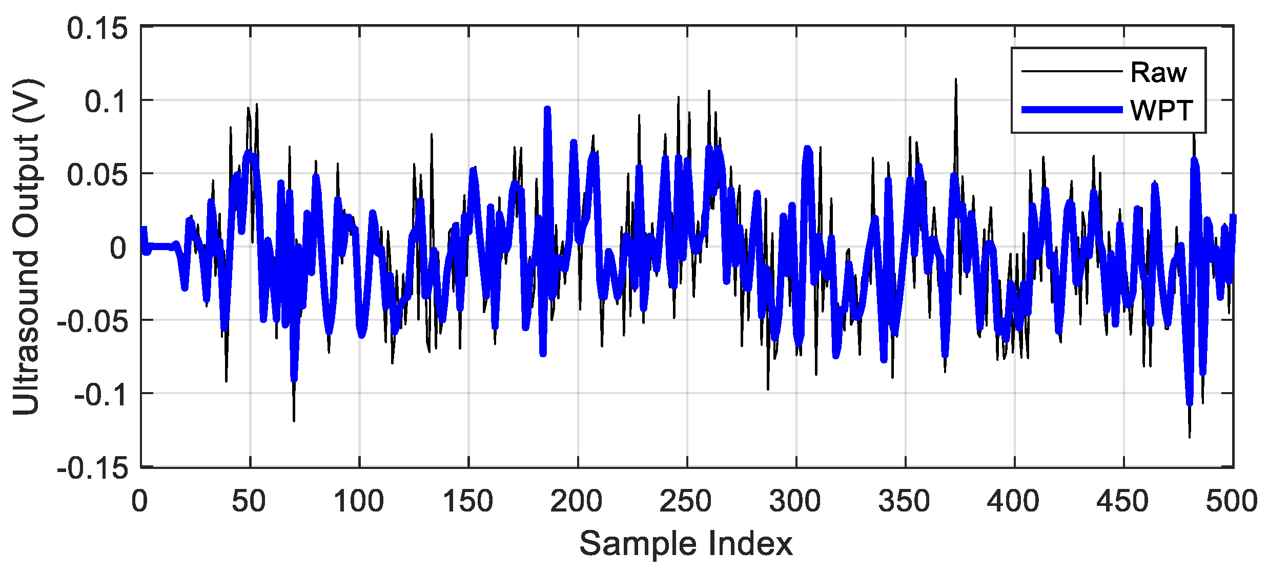
The coefficients are allocated according to their Shannon entropy and are rebuilt to generate a filtered signal. Based on a data set obtained from experimental procedures described in
Section 3,
Figure 2 describes an example of the previously mentioned procedure considering 500 recorded points, representing 10.42 ms of data acquisition with a sampling frequency of 48 kHz. In this case, coefficients can be assumed quantitatively to represent signal distributions combining their characteristics; these could be used in an efficient way for training when associated with a time series forecasting problem.
The Shannon entropy describes the energy content in a signal through the distribution of amplitude levels. The uncertainty definition is adopted in this case for probabilistic treatment purposes and can be defined as a logarithmic function
, given by
where
is the occurrence probability associated with an event
. Thus, the entropy indicates the probabilistic uncertainty of a probability distribution [
38]. After normalizing the input variables of the time series, the pertinence degree is calculated in the fuzzy layer. It corresponds to how the inputs satisfy the fuzzy sets associated with each input. In the rule layers, the firing level is calculated according to each rule.
To solve the forecasting problem, a data set is selected, and the mean, variance, and covariance values were used in the statistical analysis. The variance
of each variable can be defined as
where
is the value of the predicted output variable
in object
, and
is the mean value.
indicates how far the predicted values are from expected values. The covariance
is the linear correlation between two random variables according to the following equation:
where
also represents the value of the predicted output—now for variable
in object
—and
is the mean value. Here, the eigenvalues and eigenvectors are calculated and associated with the cumulative variability percentage in order to determine the main components (factors). Factors with the highest eigenvalues are selected, and indicators of each factor are then calculated. The influential characteristics are chosen based on the evaluation of indicators considering the most significant factors.
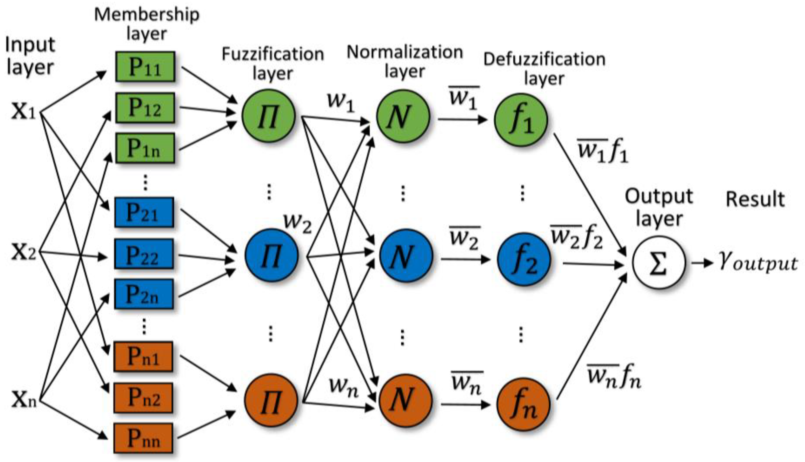
4.2. Adaptive Neuro-Fuzzy Inference System
After the filtering procedures described in the previous section, the ANFIS method was applied for mapping input characteristics with the objective of creating input rules. These rules generate a set of characteristics associated with the desired output [
39]. Considering an arbitrary selection of functions, the structures are predefined based on characteristics of the model variables [
20]. The structure of ANFIS is a combination of a fuzzy inference system and a neural network; the summary of this architecture is presented in
Figure 3.
The fuzzy inference structure considering grid partitioning creates a single-output Sugeno fuzzy system, which is used as an initial condition for ANFIS training (see
Figure 3). The grid partition method improves parallel processing performance, ensuring equality in the distribution of tasks to each core of the processor. For this type of cluster, a distinct rule is defined for each combination between the participation function and the correspondent output function [
40]. Taking into account a subtractive cluster structure, which requires a separate data set and distinct arguments, it is possible to extract the rules sets that can identify the behavior of the time series. In this type of cluster exists a specific rule for each fuzzy cluster [
41].
The fuzzy inference system based on c-means (FCM) automatically selects the number of clusters and randomly distributes the coefficients to each sample of the data set. The algorithm repeats this procedure until it reaches convergence, which means that each cluster centroid
should be calculated considering its membership level for
data points [
42].
Any point
has a set of coefficients according to the cluster
-th degree, where
represents the clustering degree, and
the fuzzy partition matrix exponent. The FCM method tries to separate elements of the data set in a finite collection assuming a predefined criterion [
43]. Thus, the objective function to be minimized, with
clusters, can be expressed by
considering
4.3. Algorithm Setup
Summarizing the technique procedures until this step, at first, a scalable filter was applied in the time series. In the sequence, a decomposition procedure was performed assuming Wavelet Packets Transform (WPT) from three to five levels. Previous tests showed that more levels did not improve the results obtained in this work [
44]. We also considered two and three nodes during decomposition, and again, previous tests reported that, when more nodes were assumed, a loss of characteristics of the original signal was reported. The decomposition was performed to obtain a wavelet package tree; after that, WPT was applied.
For the fuzzy inference structure based on grid partition, two functions were associated with each input; in this case, Gaussian functions were utilized. The Gaussian function adopted here is given by
where
is the center and
represents the spreading parameter of the Gaussian function. For the output, a linear function was used.
In the FCM structure, 5 to 30 subtractive clusters were considered in the analysis. The influence range of each center was specified in each dimension to 0.5; i.e., for each cluster center, a spherical neighborhood with a radius equal to the previously mentioned value was assumed [
14]. In order to apply standardized training procedures, the maximum number of iterations was set to 1000. Additionally, an adaptive algorithm was assumed with an initial step of 0.01, a decreasing rate equal to 0.9, and an increasing rate equal to 1.1. The hybrid neural network optimization method uses the combination of least-squares estimation and error back-propagation for training [
13].
The error signal is calculated by the difference in net target
to the net output
for both training and testing procedures. Finally, a metric of global error evaluation based on the root mean square error (
) was assumed as a stopping criterion during training and also for testing, where
This article presents other metrics for validation of the proposed method, such as mean absolute error (
and mean absolute percentage error (
).
denotes the mean of absolute difference between the observed value to the predicted one, given by:
calculates the average error ratio to the correct values, where
Based on recent studies focusing on time series forecasting [
45,
46,
47,
48], the coefficient of determination
was assumed as a performance criterion for model evaluation; see Equation (18). Thus,
is the mean of the targets
, and these values represent the observed data—those acquired using the ultrasound equipment.
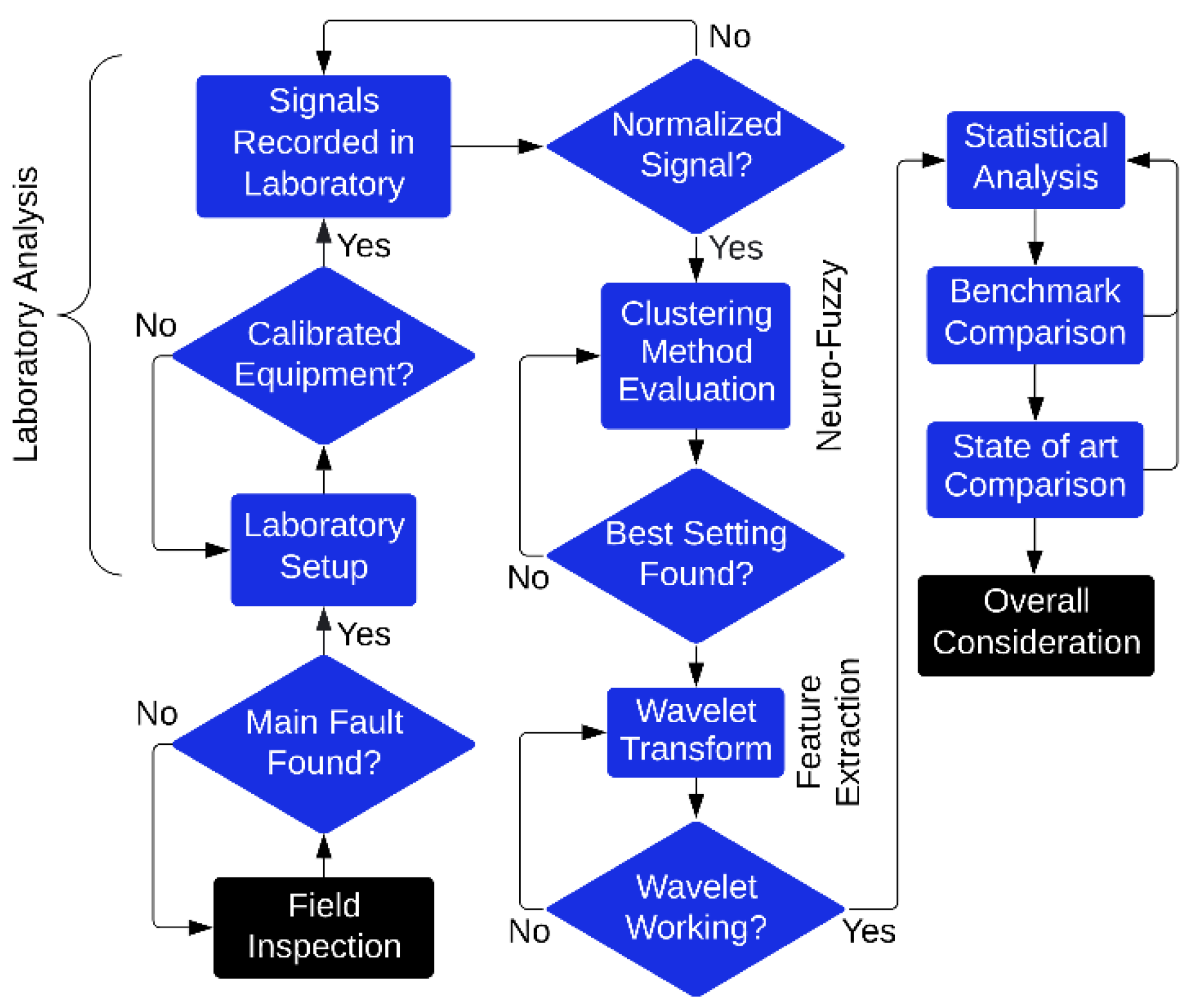
With the objective of illustrating the procedures and methods described in this research,
Figure 4 presents a flowchart of this research. The flowchart shows the analysis from the insulator which will probably develop the failure to predictability analysis.
5. Results and Discussion
Taking into account the parameters described in the previous section to configure both feature extraction and neuro-fuzzy methods, this section presents and discusses the results of the proposed model. This section was divided into four subsections: (i) analysis of the inference system; (ii) analysis of the fuzzy c-means clustering method; (iii) comparison of the proposed method with classical approaches; and (iv) a brief review about the state-of-the-art approaches that follow the same line of this research.
For the statistical analysis, the time series obtained in the experimental procedure presented in
Section 3, which was based on a contaminated insulator, was divided into five data sets of 50,000 samples each. The percentages of each data set assumed for training, validation, and testing were 75%, 15%, and 10%, respectively. The amount of data assumed for the three phases previously mentioned was obtained based on prior evaluations of the model performance in order to avoid overfitting during both validation and testing phases. The mean results provided by the algorithms among all data sets were assumed and are presented in the next subsection. Data analysis was conducted assuming the signal obtained from the wavelet energy coefficient.
5.1. Analysis of the Inference System Structure
Three fuzzy inference structures were examined in this study: the first one from data using grid partition, the second one from data assuming subtractive clustering (FCM), and the third one from data using FCM clustering.
Table 1 shows mean values considering the decomposed signal in wavelet packets until the third level, where one node was considered. In all tables, underlined results indicate the best result for each column.
As presented in
Table 1, the grid partition structure provided the fastest results for training. However, the faster the method, the lower the performance in terms of the coefficient of determination. The subtractive clustering structure provided the best results. However, it was 87.97% more time-consuming when compared to the grid partition strategy.
In all cases reported in
Table 1, the standard deviation values indicated that the three approaches are stable, even considering distinct windows in time.
Table 1 also presents the
RMSE values obtained during the testing phases of each method. By analyzing the
RMSE standard deviation of all methods, a small value was obtained, with this equal being to 7.81 × 10
−4.
MAE also provided a low standard deviation value between the analyzed methods of 3.88 × 10
−3. Finally,
MAPE values follow the trend of the
RMSE. Taking this information into account, the performance analysis presented in the sequence of this article considered the coefficient of determination as the main factor.
The FCM clustering structure is widely discussed in the specialized literature, as can be seen in [
9,
13,
14,
18]. The method provided a balanced performance when both execution time and
R2 were evaluated. In this case, the mean time was considered as one of the criteria assumed to select the best fuzzy inference structure. Due to these aspects, and the
R2 values presented in
Table 1, the method presented in the next subsection was chosen for future analysis. Additionally, distinct decomposition configurations based on wavelet packets will also be discussed. Assuming FCM clustering,
Table 2 shows an evaluation of the time and algorithm forecasting performance according to the number of clusters.
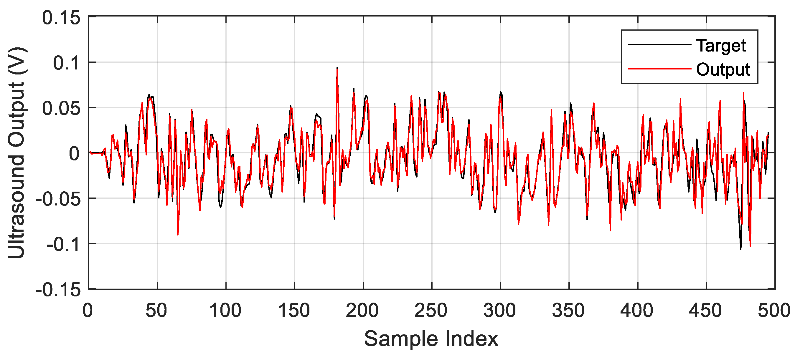
In terms of performance, it can be emphasized that the results obtained between 5 and 10 clusters. In this way, 10 clusters were used for comparison with respect to WPT configurations. In terms of execution time, a progressive increase can be observed with a proportional increase in the number of clusters. To illustrate the relation between the input (target) and the predicted (output) signals during the testing phase,
Figure 5 shows the results for 500 samples considering one-step ahead forecasting, using 10 clusters.
The , and values for the testing phase were smaller using more clusters, however the time required for convergence was longer. Again, small variations in terms of the number of clusters for and were obtained.
5.2. Analysis of the Fuzzy C-Means Clustering Method
After defining the structure of the model, this section provides an evaluation of the fuzzy c-means clustering method. The results reported in this section employed the third, fourth and fifth levels of wavelet decomposition and three nodes. The underlined results represent the best results of each configuration, while results in bold indicate the global best results.
Table 3 presents the results for the training phase. The first number in column 1 indicates the decomposition level, while the second one represents the number of nodes.
The algorithm provided the best results considering four decomposition levels and two nodes. Validation results are presented in
Table 4.
When validation results were evaluated, a similar condition when compared to the training phase was observed, where both the decomposition level and the number of nodes that provided the best results for training were replicated for validation. The same behavior was obtained during the testing phase (see details in
Table 5).
The comparison among distinct data sets during testing showed that the algorithm is stable, presenting variations in performance smaller than 0.79%. The best overall result was obtained considering the FCM clustering method with 10 clusters, with four levels and two nodes for the Data Set 3. The complete statistical analysis is presented in
Table 6, where the covariance is calculated considering the variation in terms of the number of nodes associated to each decomposition level.
The algorithm provided considerable small variance values, showing that WPT can efficiently reduce the effect of noise in the time series, providing a stable algorithm. The importance of evaluating more performance measures can be highlighted at this point, as for the , three distinct configurations provided the similar results, using two nodes. The fact of adding the metric contributes to the selection of the best model, as already described in this paragraph. The values obtained in this case helped to confirm that three levels and three nodes provided the best model configuration.
5.3. Benchmarking with Nonlinear Autoregressive Methods
Assuming the task of comparing the proposed approach with well-stablished methods for time series forecasting, in this section, we considered two more structures: a Nonlinear Autoregressive (NAR) model, and a Nonlinear AutoRegressive with Exogenous Input (NARX) model, both of which are based on Neural Networks technique [
49].
During training, three distinct classical approaches were considered: Levenberg–Marquardt (LM), Bayesian Regularization (BR), and Scaled Conjugate Gradient (SCG). Additionally, distinct configuration parameters were assumed: the number of hidden neurons (NHN), the number of regressors (ND), and the number of delayed outputs.
In the NAR network the calculation is based on Data Set 1, and in NARX networks, the calculation is based on the data relationship of Data Set 1 to Data Set 2. Data Set 2 represents values in a time window ahead of Data Set 1.
Table 7 was based on
and
Table 8 on
. These tables present the benchmark for all methods described above. Results were presented for network testing. For both hidden layers and regressors, amounts of 5, 10 and 15 were considered in the evaluation.
In this analysis, NAR and NARX methods provided lower performance when compared to the proposed Wavelet Neuro-Fuzzy approach. In its best case, the NAR model reached 0.8201 in terms of during the testing phase, which was much lower than the Wavelet Neuro-Fuzzy model, which reported 0.9700. The variation of the training method did not significantly impact the final results of both NAR and NARX models, as well as the number of hidden neurons. However, when the number of regressors was increased, an improvement in the performance associated with values could be noticed. In this case, it is important to emphasize that, by increasing the number of regressors, the computational effort also increases. After 15 regressors, the maximum number of iterations () was reached by both methods.
Based on results, NAR and NARX methods continued to maintain inferior results when compared to the proposed Wavelet Neuro-Fuzzy approach; even when varying both the settings and the optimization model, the values provided by these methods were much higher than the Wavelet Neuro-Fuzzy model.
5.4. State-of-the-Art Approaches and Comparisons
Huang, Oh and Pedrycz presented two studies in [
13] and [
14] comparing different techniques with FCM and wavelets. In the proposed evaluations, other techniques based on FCM also presented small errors. The article presented in [
13] exposed how hybrid algorithms provided superior results when compared to the application of isolated techniques. In [
14], the FCM method was used for the premise calculation, while the consequence calculation was obtained by wavelet functions whose parameters were estimated with the aid of the least square method.
Other work based in FCM was presented by Yang and Liu in [
9], where an application focusing on time series also presented interesting results. The proposed model was also based on feature extraction through wavelets. The application considered the technique proposed by [
50] for noise detection in time series. Comparisons showed that this algorithm is superior to ANFIS and the classic Artificial Neural Networks approach.
In the works reported in [
5,
19,
20], ANFIS was assumed for time series forecasting. Fu, Cheng, Yang, and Batista showed in [
20] that ANFIS provided better prediction when compared to classical approaches. Additionally, an improved Wavelet-ANFIS was proposed and the results reached
% in terms of accuracy assuming three association functions.
In [
18], Damayanti compared ANFIS and fuzzy learning vector quantization (FLVQ). The author showed that FLVQ provided better results for image classification purposes when wavelet transformation was used.
The ANFIS method was also assumed in [
15] considering two Gaussian association functions with WPT. In this study, ANFIS was adopted to classify different types of disturbance events in power quality. The method was assumed for fuzzy inference structure evaluation based on grid partition, the same evaluated in this research and reported in the first line of
Table 1. Additionally, here, the method was compared to FCM and subtractive clustering. Moreover, in [
15], promising results were obtained, and an accuracy of 99.56% was obtained for the classification task. In this case, it is important to emphasize that a considerable small data set was assumed, and the variability of the method was not evaluated. In this way, even providing interesting results, there is a lack of information about the algorithm’s precision and robustness.
Similar to the previously mentioned work, Babayomi and Oluseyi obtained an accuracy of around 81% for location and prediction for 10 different types of faults [
16]. In this case, just the ANFIS method was assumed considering grid partition.
6. Conclusions and Future Research
This article presented a complete approach for predicting electrical insulator conditions. This work was based on an experimental procedure for data acquisition using a contaminated insulator, which was removed during an inspection of an electrical system in the South Region of Brazil. Ultrasound equipment was used during the experiment and a data set was obtained. To predict the condition of the insulator, a hybrid neuro-fuzzy approach was adopted. The signal provided by the ultrasound apparatus was filtered assuming a Wavelet Packets Transform in order to improve the performance of the time series forecasting model. Additionally, three inference system structures were evaluated: grid partition, fuzzy c-means clustering, and subtractive clustering. Moreover, distinct parameters as the numbers of clusters, levels, and nodes were adjusted to improve the model performance.
The application of ANFIS for time series forecasting was shown to be a reasonable approach, considering both computational effort and performance. By assuming a larger number of clusters, a considerable increase in time (computational effort) was reported, whereas no significant improvement in the result was observed in terms of coefficient of determination.
In a specific evaluation associated with the algorithm configuration, the FCM clustering method showed balanced results in terms of training time and accuracy. This approach was successfully reported by other researchers and emphasized in this work.
The statistical analysis showed that the proposed approach provided low variability, even considering distinct data sets, confirming the method’s robustness for this application. Additionally, it can be emphasized that the method robustness was improved by the application of Wavelet Packets Transform for noise reduction and feature extraction.
Contaminated insulators are reported by energy companies as a frequent problem. Taking into account the fact that most of the energy network uses aerial lines without coverage, the application of this technique for insulator monitoring can provide interesting information, whether they are going to reach failure in a future horizon or not.
In addition, as an alternative approach to the use of a neuro-fuzzy system for time series forecasting, some authors are assuming deep learning techniques for the same purpose, as presented in [
51,
52]; for example, the Long Short-Term Memory (LSTM) method. Taking into account the fact that, in most studies, no comparisons were performed between these algorithms [
53], this approach can be suggested as interesting future work when considering the same data sets. Finally, the future of this research will be focused on the development of hardware capable of detecting defective insulators early. Additionally, by associating failure classification presented in [
44], and time series forecasting as discussed in this work, a more elaborated method to predict distinct types of failures in electrical insulators can be developed. The idea for future works is to combine both models focusing on the development of a specialized system capable of both to predict and classify failures as cracks, contamination among others.

 ,
, 


